Dynamic dissipative solitons in nematics with positive anisotropies

Abstract

Electric field induced instabilities of nematic molecules are of importance for both fundamental science and practical applications. Complex electro-hydrodynamic (EHD) effects such as electro-convection, fingerprint textures, spatiotemporal chaos, and solitons in nematics have been broadly investigated and generated much attention. In this work, dissipative solitons as a novel EHD phenomenon are realized in nematics with positive anisotropies, presumably for the first time. Unlike the ones reported recently in nematics with negative anisotropies whose formation and dynamics are mainly attributed to the flexoelectric and electro-convection effects, the solitons discussed here arise from the nonlinear coupling between the director field and the isotropic flow induced by ion motion. The structure and dynamics of the solitons are demonstrated and the influences of chirality, azimuthal anchoring and ion concentration are also investigated. Finally, we show that the propagation trajectory of solitons can be manipulated by patterned photoalignment and micro-particles can be trapped by them as vehicles for micro-cargo transport.

---

Introduction

Nematic liquid crystals (LCs) are self-organized anisotropic fluids with a long-range orientational order of molecules defined by the director, n.¹ For several decades, research has been focusing on the dynamic response of LCs to electric fields, which led to the revolutionary development of liquid crystal displays (LCDs). An elementary unit, or a pixel, of a traditional LCD is composed of two glass substrates coated with a transparent electrode and a nematic LC confined between them. Reorientation of the director n, which also exemplifies the optic axis, can be induced by applying an electric field across the cell, leading to the modulation of the macroscopic refractivity. Such a behavior originates from the anisotropic properties of LC molecules, such as the dielectric permittivity and electrical conductivity, i.e., the permittivity (ε_‖′) and conductivity (σ_‖) measured along n are different from those (permittivity, ε_⊥′, and conductivity, σ_⊥) measured perpendicular to n. The strong coupling between the reorientation of n and the fluid velocity also enables nonlinear responses such as electro-convection (EC)² and solitons (solitary waves).³

Solitons are localized travelling waves that were first discovered in a shallow canal by Russell in 1834.⁴ They are ubiquitous and exist in various areas of physics, such as nonlinear photonics, magnetic matter, superconductors and also LCs.⁵ However, solitons of higher dimensions supported by the standard cubic nonlinearity suffer from severe instabilities.⁶ Generation of multidimensional solitons and manipulation of their mobility are still grand challenges in the science of nonlinear physics and materials. Studies on solitons in LCs have been carried out for over five decades. Most early studies^7–11 were concerned with “walls” in nematics, also referred to as planar or linear solitons,¹² generated by magnetic or electric fields, which actually are transition regions where n smoothly reorients by π. By rotating magnetic fields, a variety of interesting solitons were subsequently observed.^13–15 Due to the birefringence of LCs, optical solitons in nematic LCs, called nematicons, have received much attention. They represent self-focused, continuous wave light beams and have promising applications in optical information technology.¹⁶ Topologically structured three-dimensional (3D) solitons in the form of torons or hopfions can be generated in cholesteric LCs by utilizing electric fields^17–19 or laser tweezers.^20–22 They are basically static but can also perform squirming motion driven by electric fields.^23,24 They enable twist in all three spatial dimensions and are stabilized by strong energy barriers associated with the nucleation of topological defects.²⁰

Recently, multidimensional dissipative solitons driven by electric fields were observed in nematics.^25–28 These solitons represent spatially-confined director perturbations driven by electric fields that propagate rapidly through a slab of a homogeneously aligned LC and survive collisions with each other. So far, these solitons are only confirmed in LCs with a negative dielectric anisotropy, i.e., Δε′ = ε_‖′ − ε_⊥′ < 0 and a relatively small positive, or negative, conductivity anisotropy, Δσ = σ_‖ − σ_⊥. It was indicated that they cannot exist in a LC with positive Δε′.²⁷ This was anticipated from the fact that a positive dielectric anisotropy Δε′ will induce a dielectric torque which strongly inhibits the flexoelectric torque at high amplitudes of electric fields. In addition, the positive Δε′ will also lead to a direct Freedericksz transition where space charges cannot form according to the Carr–Helfrich electro-convection (EC) mechanism.^29,30 According to the reports,^25–28 both flexoelectric effect and space charges are the elementary conditions for the formation of these dissipative solitons. Such stringent conditions on the LC material (negative Δε′ and small positive or negative Δσ) would greatly limit broader research of these novel solitons, which are very important not only theoretically for nonlinear physics but also for practical applications such as targeted 2D delivery of optical information or mass transport via micro-cargos.

In this work, dynamic dissipative solitons are successfully generated in nematic E7 with positive Δε′ and Δσ. E7 is a standard liquid crystal, which has been broadly used in laboratories and industry worldwide. The nematic material is confined in cells spin-coated with a sulfonic azo dye SD1 and processed by the photoalignment technique.³¹ In contrast to the conventional rubbing technique, photoalignment not only avoids problems such as mechanical damage, electrostatic charge, or dust contamination, but also produces high-resolution multidomain alignment.^32,33 Instead of forming a quasi-homeotropic state (Freedericksz transition) as predicted by the standard model (SM)³⁴ or some complicated EC patterns as reported in ref. 35, dynamic dissipative solitons are observed. The formation mechanism roots in the strong coupling between n and the isotropic flow induced by ion motion, which is allowed by the relatively weak azimuthal anchoring strength of the photoaligned surfaces as well as the relatively high ion concentration of the sample due to a weak dissolution of the SD1 layers with time. The solitons are waves of director deformations that oscillate with the frequency of the applied alternating current (AC) electric field and can be observed in situ through polarizing optical microscopy (POM). The dynamics of the solitons was analyzed and tracked, and exhibited a wave-particle dualism. They can either pass through each other like waves or collide with each other and reflect like particles, a behavior which depends on the amplitude (E) and frequency (f) of the applied electric field. The influence of chirality on these solitons was further investigated by doping E7 with a chiral dopant. It is shown that the trajectories of moving solitons can be manipulated by a predesignated alignment pattern and micro-cargos, such as silica particles, can be attracted and transported by the solitons. Finally, the contribution of the weak azimuthal anchoring and the influence of ion concentration are demonstrated.

Results

Experimental setups

The nematic LC we used as the soliton medium is E7 with a positive dielectric anisotropy of Δε′ ∼ 12 and a positive conductivity anisotropy of Δσ ∼ 10⁻⁷ Ω⁻¹ m⁻¹ (measured at 1 kHz, 50 °C). The nematic is aligned homogeneously in cells with thickness d ∼ 11 ± 3 μm. The homogeneous alignment is realized by the photoalignment technique, in which substrates, spin-coated with SD1, are exposed to linearly polarized ultra-violet (UV) light. Either a sinusoidal or a rectangular AC field E = (0, 0, E) is applied along the z axis (perpendicular to the xy substrate plane of the cell, Fig. 1) so that the sandwich cell acts as a plate capacitor. The sample is placed on a hot stage with its alignment direction, m, parallel to the x axis, and observed through a polarizing optical microscope (POM) with crossed polarizers (the polarizer and analyzer are parallel to the x and y axes, respectively). More details about the experimental part can be found in the Experimental section of the ESI.†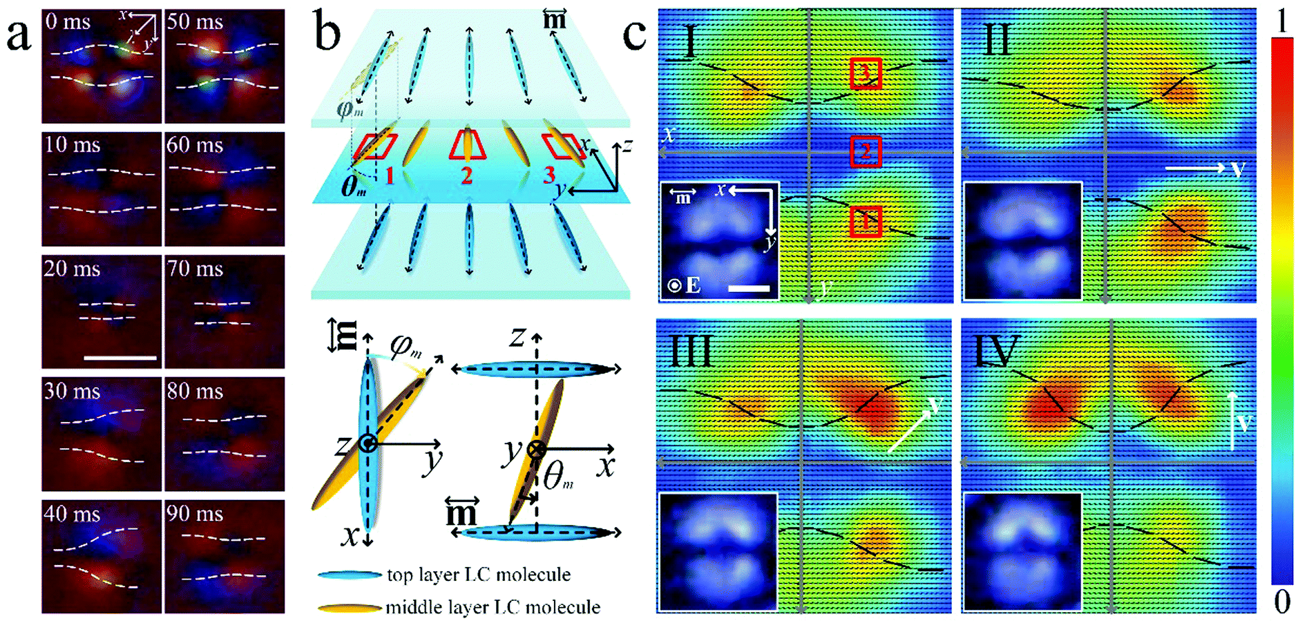

Fig. 1 The structure of solitons. (a) POM micrographs of a soliton modulated by a rectangular AC field of E ∼ 0.4 V μm⁻¹, f = 10 Hz. White dashed lines represent the director field. λ represents the slow axis of the red plate. Both polarizer and analyzer are parallel to the x and y axis, respectively. Scale bar 20 μm. (b) The schematic structure of a soliton. m represents the alignment direction. φ_m and θ_m represent the azimuthal angle and the polar angle of the local mid-layer director. (c) Transmitted light intensity maps and the corresponding mid-layer director fields (black dashed lines) in the xy plane within solitons. Rectangular AC field E ∼ 0.7 V μm⁻¹, f = 20 Hz. v represents the velocity of the soliton. The color bar shows a linear scale of transmitted light intensity. Insets are the corresponding POM micrographs, scale bar 10 μm. Both polarizer and analyzer are parallel to the x and y axis, respectively. Red squares 1, 2, and 3 are corresponding to the ones in (b).

The structure of solitons

Independent “frog-egg-like” solitons are randomly generated in the nematic LC as E increases above some frequency-dependent threshold (E_N). Outside the solitons, the sample shows a homogeneous dark state. Rotating the sample by a small angle, a periodic change of light intensity (monochromatic light source) is observed (Fig. S1, ESI†). This suggests that at low frequency f, due to the dielectric toque and its relaxation, the middle layer of n oscillates with f out of the xy plane by a polar angle θ_m with respect to the z axis (Fig. 1b). θ_m can be estimated from the dependence of transmitted light intensity on the polar angle, which changes from ∼66° to ∼70° periodically (Fig. S1, Experimental section, ESI†). In the xy plane, the projection of n onto the xy plane aligns along m. Inside the solitons, the light intensity increases, indicating azimuthal deviations of n from m. To identify the sign of the azimuthal angle (φ_m with respect to the x axis, Fig. 1b), a first-order red plate compensator (530 nm) is inserted between the sample and the analyzer, with the slow axis λ making 45° with the analyzer. Either yellow or blue can be distinguished due to the subtractive or additive effect of the phase retardations of the compensator and the nematic.³⁶ By observing the solitons through a higher frame rate at 100 fps, a frequency-dependent modulation of n is determined (Fig. 1a), which may be induced by the flexoelectric effect. Simultaneously, n is oscillating out of the xy plane with the polar angle θ_m due to the dielectric effect. It is also found that these solitons can move either parallel or perpendicular to m, which depends on their director structures. Fig. 1c shows the time-averaged structure of the solitons observed at a lower frame rate 10 fps. Solitons with a time-averaged mirror-symmetry director structure are relatively static (Fig. 1c(I)). As long as this symmetry is broken, which can be induced by factors such as background flows or local director distortions, the solitons start to move. Solitons propagating along the x-axis lack the symmetry with respect to the y-axis (Fig. 1c(II)). Vice versa, solitons propagating along the y-axis lack the symmetry with respect to the x-axis (Fig. 1c(IV)). A more severe deformation of n in region 3 also can lead to an oblique motion with respect to the x-axis (Fig. 1c(III)). Additionally, the time-averaged director structure of the solitons shows a static biconcave structure. This may be attributed to the longer duration of the biconcave deformation in one period of director oscillation as observed in Fig. 1a. The size of the solitons is mainly dependent on the cell gap, d (Fig. S2, ESI†). Both the width (w_N) and length (l_N) of the solitons increase with d.

Generation and dynamics of solitons

As we suggested above, these dissipative solitons are driven by external AC electric field. Fig. 2a shows the threshold dependences of different states of the sample on f. Basically, the nematic firstly experiences a Freedericksz transition from the homogeneous state (inset I) to a quasi-homeotropic state where reverse-tilt domains (TIDs, inset II) are observed. These TIDs are transient and will eventually annihilate within several minutes. The threshold of the Freedericksz transition (E_F) is about 0.1 V μm⁻¹, independent on the frequency. The solitons (inset III) emerge after the Freedericksz transition and show a frequency-dependent E_N, which is proportional to f^1/2 (left-top inset). This square-root dependence of E_N on f is observed in almost all the samples throughout our experiment, which indicates that the soliton is caused by an isotropic electro-hydrodynamic (EHD) instability.^37–39 Such an interpretation is supported by the circular motion of tiny suspended dust particles observed both in the nematic and the isotropic phase at E_N.^37–40 On further increase of E, periodic domains (inset IV) that extend gradually and eventually cover the entire electrode area of the cell, are observed. Just like the dissipative solitons observed in nematics with negative dielectric anisotropy,^25,26 the ones here also show electric field dependent dynamics. Both the amplitude and the direction (either parallel or perpendicular to m) of the velocity (v) of the solitons can be tuned electrically (Fig. 2b and Movie S1, ESI†). At f = const, the amplitude of soliton velocity (v) increases with E.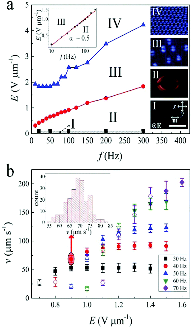

Fig. 2 Soliton properties as a function of electric field. (a) Threshold dependence of different states (I homogeneous state, II quasi-homeotropic state, III soliton state, IV periodic domains) on the frequency of rectangular AC electric fields, f. Insets are the POM micrographs corresponding to different states (I: E = 0 V μm⁻¹; II: E ∼ 0.2 V μm⁻¹, f = 20 Hz; III: E ∼ 0.7 V μm⁻¹, f = 20 Hz; IV: E ∼ 2.2 V μm⁻¹, f = 20 Hz). m represents the alignment direction. E represents the electric field which is perpendicular to the xy plane. Both polarizer and analyzer are parallel to the x and y axis, respectively. Scale bar 50 μm. The inset on the top-left corner shows the square-root dependence of the threshold of solitons, E_N(f), with α being the slope of this dependence. (b) Dependence of the amplitude of velocity, v, of solitons on the amplitude of a rectangular AC electric field, E. The solid and hollow symbols represent the velocities parallel and perpendicular to m, respectively. The error bars are calculated from the standard deviation of velocities of different solitons at the same electric field. The inset represents the velocity distribution of solitons at f = 40 Hz, E ∼ 0.9 V μm⁻¹.

Generally, the solitons form randomly throughout the nematic bulk (Fig. 3a(i)). This may be attributed to the instabilities induced by the motion of ions since weak flow patterns are observed during the formation. With the formation and motion of solitons, these flow patterns will subsequently disappear (Movie S2, ESI†). The explanation of soliton formation via ions can be further supported by the phenomenon described below. In the experiment, we first increase E above E_N to generate solitons. At an arbitrary time, E is decreased below E_N and the solitons instantly disappear. If we increase E above E_N within ∼10 s, it is found that the solitons are generated at almost the same location before the decrease of E. However, once the interval is longer (such as 30 s), new solitons are randomly generated in space. Taking a typical diffusion coefficient of ions in LCs of 2 × 10⁻⁹ m² s⁻¹, the delocalization of ions is about 20 s,²⁷ which is consistent with our observation. Strong EHD flows can induce the solitons, too (Fig. 3a(ii) and Movie S2, ESI†). These flow patterns are usually observed at the edges of the cell or nearby disclinations. The solitons also nucleate near disclinations (yellow dashed line, Fig. 3a(iii)) and at irregularities, such as dust particles (Fig. 3a(iv)). One soliton can even split into two or more solitons (Fig. 3a(v)), which accompanies the elongation of the soliton. The elongation process results in a continuous accumulation of excess elastic energy, and the soliton fractionates when the energy penalty from the elastic deformation cannot be compensated by the effects of surface and dielectric interaction.²⁷ Furthermore, the collision of two solitons may also lead to the generation of new solitons (Fig. 3a(vi)). More details about the nucleation of solitons can be found in Movie S2 (ESI†).

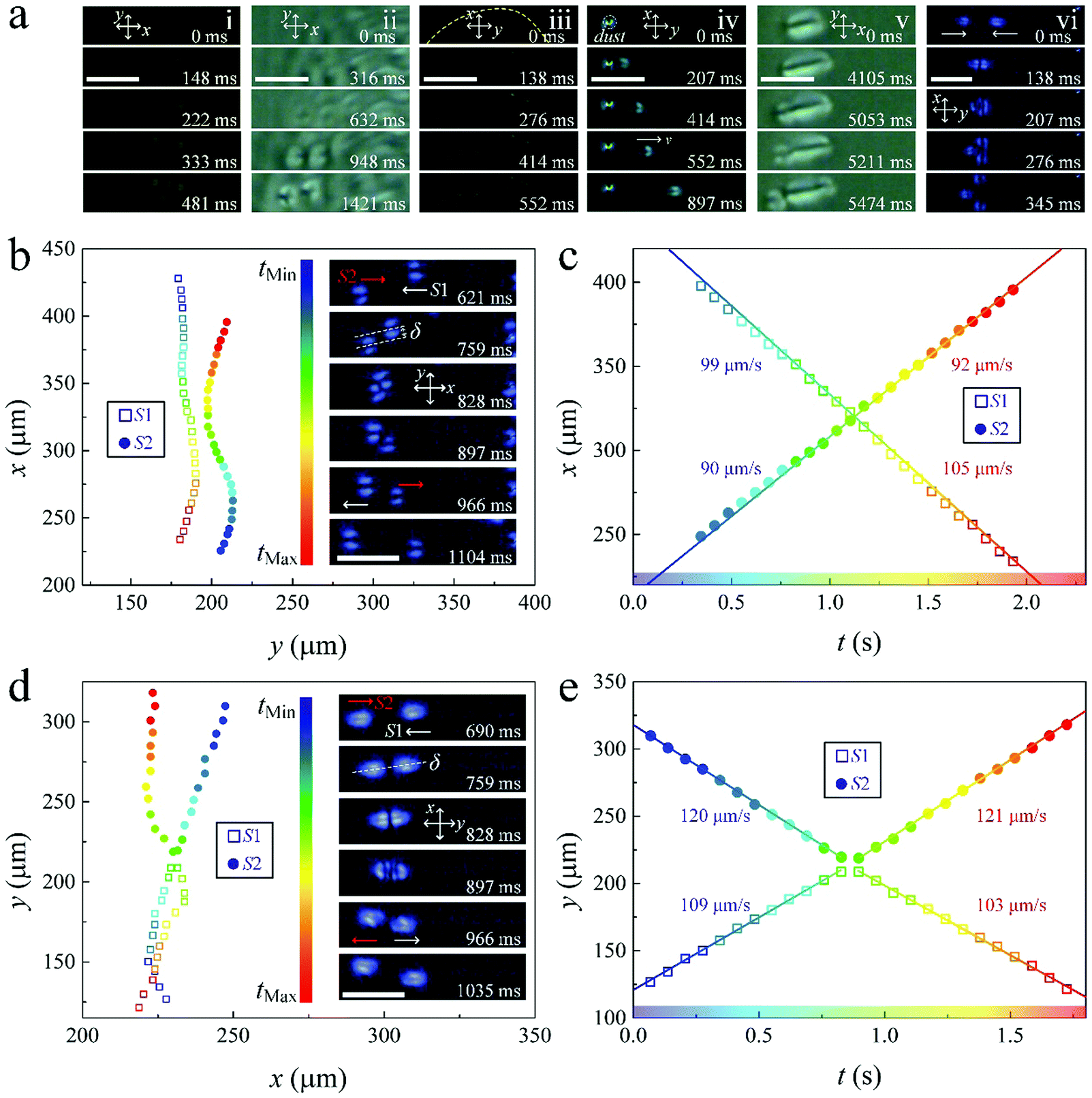Fig. 3 Nucleation and interaction of solitons driven by rectangular AC fields. (a) random generation of solitons (E ∼ 0.7 V μm⁻¹, f = 20 Hz) (i), EHD flows induce solitons (E ∼ 0.6 V μm⁻¹, f = 20 Hz) (ii), nucleation of solitons adjacent to a disclination (yellow dashed line) (E ∼ 0.7 V μm⁻¹, f = 20 Hz) (iii), nucleation of a soliton at a dust particle (E ∼ 1.2 V μm⁻¹, f = 70 Hz) (iv), proliferation of a soliton (E ∼ 0.5 V μm⁻¹, f = 20 Hz) (v) and collision of two solitons creates a new soliton (E ∼ 1.2 V μm⁻¹, f = 70 Hz) (vi). (b) The trajectories of two solitons pass through each other. E ∼ 1.1 V μm⁻¹, f = 40 Hz. The color bar represents the elapsed time. t_Min = 0 s, t_Max ∼ 2.0 s, time interval Δt ∼ 0.069 s. Insets are the POM time series micrographs of the solitons. δ represents the offset between the centers of two solitons before the collision. (c) Time dependence of x coordinates of the solitons in (b). (d) The trajectory of two solitons colliding and reflecting into opposite directions; E ∼ 1.2 V μm⁻¹, f = 60 Hz. The color bar represents the elapsed time. t_Min = 0 s, t_Max ∼ 1.8 s, time interval Δt ∼ 0.069 s. Insets are the POM time series micrographs of the solitons. δ represents the offset between the centers of two solitons before the collision. (e)Time dependence of the y coordinates of the solitons in (d). In figures (a), (b) and (d) the polarizer and analyzer are parallel to the x and y axis, respectively, with the scale bars indicating 50 μm.

The solitons show a wave-particle dualism during collisions with each other, which depends on the degree of offset, δ (the distance between the centers of the two solitons) as well as their motion direction (Fig. 3b–e and Movie S3, ESI†). When the solitons propagate parallel to m, they behave more like waves. If δ is large enough (0.5w_N < δ < w_N,), the two solitons pass through each other with little influence on their structure and dynamics (Fig. 3b and c). On the other hand, when the solitons move perpendicular to m, they behave more like particles. Especially when δ < 0.5w_N, the two solitons collide and then reflect into opposite directions (Fig. 3d and e). Such a behavior may be attributed to the increased mismatch of the director field between solitons which depends on the structure of the solitons and the offset, δ, between them.

Dissipative solitons in CLCs

The influence of chirality on the structure and dynamics of solitons was also investigated. Fig. 4a shows the director structure of a CLC soliton which changes periodically with f. It shows a torus-like structure (0 ms and 50 ms) which looks similar to the topological soliton called “hopfion”.⁴¹ In the middle layer of the soliton, the structure is skyrmion-like.²⁰ In the center, n tends to be parallel to E due to the positive Δε′, and twists by π in outward radial directions matching the quasi-homeotropic director n in the far field outside the structure. However, unlike the topological soliton reported in confinement-unwound CLCs,^19,42 whose stability is protected by the competition between the soft perpendicular boundary conditions (homeotropic alignment) and the helicoidal structure of CLC, the ones reported here are dissipative solitons whose existence requires an external electric driving field; below a certain field amplitude E, they vanish. Fig. 4b shows the E dependence of different states of the sample on f. The CLC firstly experiences a Freederickz transition which results in the fingerprint textures (inset II).⁴³ By increasing E, the fingerprint textures gradually disappear due to the unwinding effect (inset III). The CLC solitons appear after the unwinding of helixes (inset IV). Just as for achiral nematics, the threshold of CLC solitons (E_CLC) also shows a square-root dependence on f. Further increase of E results in the observation of a periodic domain that covers the entire sample (inset V). The velocity (both direction and amplitude) of the CLC solitons is also dependent on the electric field (Fig. 4c). At f = const, v increases with E. It is observed that in contrast to the bidirectional propagation of solitons in achiral nematics, the propagation of the CLC solitons is more unidirectional (Movie S1, ESI†), which is similar to the schools of skyrmions in CLCs reported recently.²⁴ However, unlike the schooling motion which is a collective phenomenon relying on the inter-skyrmion interactions, the unidirectional motion of our CLC solitons is more likely attributed to the local background flows. The dielectric oscillation of n as well as the motion of ions induces flows that break the symmetric structure of the solitons, and initiate their translation through the sample. The reason why the achiral solitons do not show such a unidirectional motion is not clear, but may be due to the different director structure (although the unidirectional motion of the achiral solitons can actually be induced by applying a different AC field which is additionally modulated with a higher modulation frequency f_m, such as f_m = 50 Hz, f = 10 Hz, Movie S4, ESI†). These flows are dependent on the local director field and can be very different in different regions. As can be seen in Movie S4 (ESI†), two crossed disclinations divide the region into four sub-regions. The background flow in each region is perpendicular to the one nearby, leading to a fascinating circular motion of solitons. The nucleation of CLC solitons is similar to the achiral ones’ (Fig. S3 and Movie S5, ESI†), and they also show the wave-particle dualism during collisions (Fig. S4 and Movie S6, ESI†). One distinct difference between the chiral and achiral systems is that, the diameter (D) of the chiral solitons shows a dependence on E, which gradually decreases with increasing E (Fig. S5, ESI†).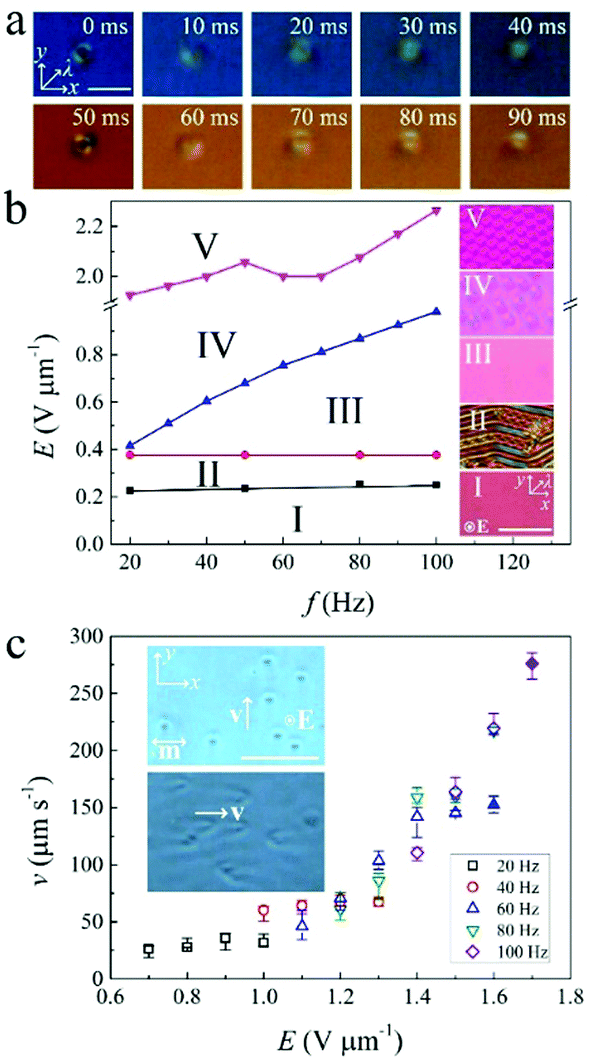

Fig. 4 Solitons in CLCs. (a) POM micrographs of a soliton modulated by a rectangular AC field with E ∼ 0.5 V μm⁻¹, f = 10 Hz. λ represents the slow axis of the red plate. Both polarizer and analyzer are parallel to the x and y axis, respectively. The scale bar is 20 μm. (b) Threshold dependence of different states (I homogeneous state, II fingerprint texture, III unwinding state, IV soliton state, V periodic domain) on the frequency of rectangular AC electric fields, f. Insets are the POM micrographs corresponding to different states (I: E = 0 V μm⁻¹; II: E ∼ 0.3 V μm⁻¹, f = 50 Hz; III: E ∼ 0.6 V μm⁻¹, f = 50 Hz; IV: E ∼ 0.8 V μm⁻¹, f = 50 Hz; V: E ∼ 2.1 V μm⁻¹, f = 50 Hz). E represents the electric field which is perpendicular to the xy plane. λ represents the slow axis of the red plate. Both polarizer and analyzer are parallel to the x and y axis, respectively. Scale bar 50 μm. (c) The dependence of the amplitude of soliton velocity, v, on the amplitude of the rectangular AC electric field, E. The solid and hollow symbols represent the velocities parallel and perpendicular to the alignment direction, respectively. The error bars are calculated from the deviation of velocities of different solitons at the same electric field. The insets show the POM micrographs of solitons travelling perpendicular (f = 60 Hz, E ∼ 1.2 V μm⁻¹) and parallel (f = 60 Hz, E ∼ 1.6 V μm⁻¹) to the alignment direction, m, respectively. The electric field E is perpendicular to the xy plane, and v represents the velocity of the solitons. Scale bar 100 μm. Both polarizer and analyzer are parallel to the x and y axis, respectively.

Cargo transport and trajectory manipulation

It has been reported that distorted LC regions, such as topological defects, can attract colloidal particles.⁴⁴ Since the solitons are actually self-confined director deformations, we here confirm that they too can attract particles. In Fig. 5a, an aggregate of two micro-particles is attracted by a soliton nearby and trapped in its center (Movie S7, ESI†). Besides, the solitons can even be used as vehicles for micro-cargo transport. In Fig. 5b, a micro-particle is carried by a soliton and moved through the nematic liquid crystal (Movie S7, ESI†). Furthermore, the propagating trajectory of the solitons can be controlled by the alignment of the cell substrates. In Fig. 5c, the nematic is divided into two regions with different alignment directions perpendicular to each other. In each region, the solitons move either parallel or perpendicular to m, depending on the applied electric field. Once a soliton crosses the boundary of the two regions, it will transform its structure and switch its moving direction to fit the new alignment direction (Movie S6, ESI†).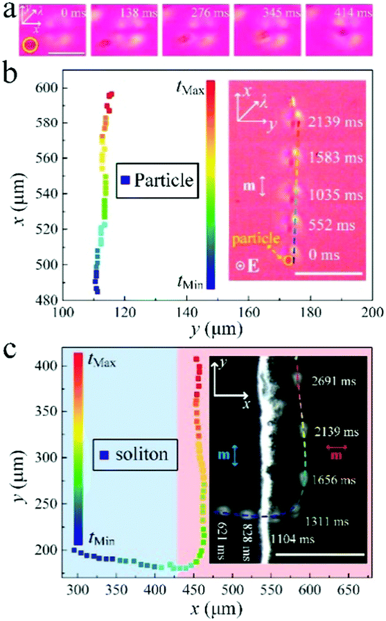

Fig. 5 Particle trapping, cargo transport and trajectory manipulation. (a) POM time series micrographs of an aggregate of two micro-particles being trapped by a soliton (rectangular AC field E ∼ 0.5 V μm⁻¹, f = 20 Hz). λ represents the slow axis of the red plate. Both polarizer and analyzer are parallel to the x and y axis, respectively. Scale bar 20 μm. The yellow circle represents the aggregate of the two micro-particles. (b) Trajectory of a micro-particle transported by a soliton (rectangular AC field E ∼ 0.9 V μm⁻¹, f = 40 Hz). The color bar represents the elapsed time. t_Min = 0 s, t_Max ∼ 2.5 s, time interval Δt ∼ 0.069 s. The inset shows the micrograph of the micro-particle transported by a soliton. m represents the alignment direction. The electric field E is perpendicular to the xy plane. The scale bar is 50 μm. λ represents the slow axis of the red plate. Both polarizer and analyzer are parallel to the x and y axis, respectively. (c) Trajectory of a soliton travelling through the boundary of two regions with perpendicular alignment. The rectangular AC field is of amplitude E ∼ 1.1 V μm⁻¹ and frequency f = 60 Hz. The color bar represents the elapsed time. t_Min = 0 s, t_Max ∼ 3.4 s, time interval Δt ∼ 0.069 s. The inset shows the micrograph of the soliton. m represents the alignment direction. Scale bar 100 μm. Both polarizer and analyzer are parallel to the x and y axis, respectively.

Discussion

Early studies on EHD instabilities in LCs have been focused on EC effects in nematics with opposite signs of anisotropies, e.g. negative Δε′ and positive Δσ,⁴⁵ where EC rolls, such as “Williams domains”⁴⁶ and “chevrons”,⁴⁷ are observed. In their case the destabilization is attributed to the charge separation mechanism introduced by Carr²⁹ and Helfrich,³⁰ which was later extended to a three dimensional theory, i.e. the standard model (SM).³⁴ Nonstandard EC effects may arise in nematics with both negative Δε′ and Δσ, but most of them can be explained by adding flexoelectricity effects to the SM.^48,49 The SM predicts no EHD instabilities in nematics with both positive Δε′ and Δσ. However, complex EC patterns, such as fingerprint textures,³⁷ Maltese crosses³⁷ and cellular patterns,³⁵ have been observed for homeotropic anchoring condition. Various explanations, such as charge injection (known as Felici–Benard mechanism),^50,51 isotropic flows,^37–39 flexoelectricity and surface-polarization effects^52,53 were proposed to account for the origin of the instabilities. However, a rigorous explanation of the formation is not available yet. On the other hand, in the case of homogeneous alignment, stationary Williams domains exist for small values of Δε′ (normally 0 < Δε′ < 0.4) only, when the threshold of the EHD instability is lower than the threshold of the Freedericksz transition.^54–57 For large values of Δε′ (just as it is the situation in our case), EHD instabilities are not expected, and only a homogeneous splay Freedericksz transition is predicted.⁵⁸ However, EC patterns in the form of fingerprint textures and cellular patterns were in fact observed in ref. 35, but the authors did not give a convincing explanation for their formation.

The EHD instabilities as a form of dynamic dissipative solitary waves has been reported only very recently and only in nematics with negative Δε′.^25–28 Their formation was attributed to flexoelectricity²⁵ and space charges.²⁷ It was not expected that such solitons can also exist in nematics with positive Δε′ since both factors are inhibited. The reason for the generation of solitons in our experiment is attributed to special conditions, namely a relatively high ion concentration in combination with weak azimuthal anchoring. The high concentration of ions induces stronger isotropic flows. These flows are the prerequisite for the solitons’ generation, as they break the stability of the system (Fig. 3a). The weak azimuthal anchoring allows the periodic azimuthal oscillation of n in the xy plane and thus keeps the structure of the solitons from collapsing.

To demonstrate the influence of the azimuthal anchoring on the generation of solitons, commercial cells coated with rubbed polyimide and filled with E7 were additionally tested. It is well known that rubbed polyimide layers provide strong azimuthal anchoring for thermotropic LCs, which is of the order of 10⁻³ J m⁻² for E7.⁵⁹ In contrast, the azimuthal anchoring of the photoalignment layer (SD1) in our experiment is only ∼2.2 × 10⁻⁵ J m⁻² according to our measurement (Fig. S6, Experimental section, ESI†). By applying an AC field to the commercial cell, it goes through a Freedericksz transition at low E and keeps a quasi-homeotropic state at high E. At low f, by rotating the sample by a small angle with m deviated from the x-axis, a periodic change of light intensity is observed, which is due to the oscillation of n out of the xy plane. The tilting angle θ_m is estimated from the dependence of the light intensity on the polar angle, which changes with f from ∼67° to ∼72° (Fig. S1, Experimental section, ESI†). No EHD instability effect is observed after the Freedericksz transition. On the other hand, E7 is also filled into a cell spin-coated with polyvinyl alcohol (PVA) solution and rubbed with velvet. It has been reported that rubbed PVA provides a relatively weak azimuthal anchoring of the order of 10⁻⁵ J m⁻²,⁶⁰ which is a value comparable to our photoalignment layer. By applying an AC field to the sample, solitons are observed after the Freedericksz transition. However, unlike the ones in the cells processed by photoalignment, the ones in the PVA cell cannot move efficiently, instead, they look like they are trapped and can only vibrate locally (Movie S8, ESI†). This may be due to the poor rubbing alignment, dust contamination, and static electric effects produced during the rubbing process.

The influence of ion concentration is also investigated by doping different concentrations of an ionic dopant (ASE2, Fig. S7a, ESI†) into E7. We estimate the ion concentration by measuring the conductivity σ_⊥ and the dielectric loss ε_⊥′′ of the sample (Fig. S8a, ESI†); the higher σ_⊥ and ε_⊥′′, the higher the ion concentration.⁶¹ E7 doped with 0 wt%, 0.1 wt% and 0.5 wt% ASE2, respectively, were filled into commercial cells (rubbed polyimide), and solitons are observed in the sample doped with 0.5 wt% ASE2 (Fig. S8b, ESI†). It should be noted that the solitons are only observed at the edges of the ITO electrodes (Movie S8, ESI†), which may be due to the stronger EHD instabilities there. At higher E, periodic EC rolls whose wave vector are parallel to the rubbing direction are observed as reported in ref. 35.

Moreover, we also find that the ion concentration of the samples processed by photoalignment technique changes with time. Both σ_⊥ and ε_⊥′′ increase greatly within a time period of 3 days (II) and then remain saturated (III, 10 days later) (Fig. S9a, ESI†). The increase of ion concentration could be attributed to a weak solubility of SD1, which is an ionic material, in the LC E7 (Fig. S7b, ESI†). The influence of such an increase is discussed below. As mentioned before, the solitons randomly form in space as long as E surpasses E_N which is attributed to the instabilities induced by ionic motion. The distribution of the ion concentration throughout the sample is not homogeneous, the regions with higher ion concentration generate solitons more easily, which means that E_N in different regions is slightly different (generally the difference is smaller than 0.1 V μm⁻¹). To eliminate this difference, we confine our measurement to the same region (770 μm × 409 μm). In Fig. S9b (ESI†), it is found that in the usual case (I, 0 days), the solitons firstly nucleate in the vicinity of a dust particle (inset), with most part of the region exhibiting no solitons. By slowly increasing E (∼0.02 V μm⁻¹ per 30 s), the number of the solitons increases gradually mainly due to the random generation and proliferation effect (Fig. 3a), and the solitons gradually fill up the region. It should be noted that the reason why we do not use the number density of solitons to represent the covered area is because the solitons generate randomly and inhomogeneously, i.e. the number density of soliton changes greatly in different sub-regions. The amount of solitons reaches the maximum at ∼1.05 V μm⁻¹ and then gradually decreases. In contrast, after 3 days (II), it is found that when E surpasses E_N, the solitons generate homogeneously throughout the region and the densities of solitons in different sub-regions are similar to each other. This may be caused by the increase of the overall ion concentration of the sample diminishing the differences among different sub-regions. By increasing E, more solitons generate in a rather narrow range of E and the amount of solitons reaches a maximum at ∼0.65 V μm⁻¹. The maximum is almost twice as large as the one in case I. Further increase of E, causes the amount of solitons to decrease gradually and finally reach saturation. It is also found that the threshold E_N decreases by ∼0.1 V μm⁻¹. Such a decrease may be attributed to the increase of the ion concentration, and can be found throughout the sample. In Fig. S10 (ESI†), the E_N of a region nearby the edge of the ITO electrode is also found to be decreased, but with a smaller amplitude.

To further verify that the formation of solitons arises from the properties of the photoalignment, and is not a privilege of E7 alone, 5CB (4-cyano-4′-pentylbiphenyl), another well-studied LC which has been broadly used both in laboratories and industry, is filled into a cell spin-coated with SD1 and processed by photoalignment. Just as for E7, both Δε′ and Δσ of 5CB are positive.²³ Dissipative solitons are observed at E above E_N, and the E_N(f) also shows the before observed square-root dependence (Fig. S11b, ESI†). Besides, it is found that the behavior of the solitons in 5CB is similar to case II of E7 (Fig. S9, ESI†), which may be attributed to a higher ion concentration of 5CB (Fig. S11a, ESI†).

Conclusion

In summary, dynamic dissipative solitons are realized in nematics with both positive dielectric and conductive anisotropies. The structure and dynamics of the solitons are demonstrated and the influences of chirality, azimuthal anchoring and ion concentration are investigated. The underlying mechanism of the formation of the solitons is still not very clear and requires further experimental and theoretical investigations.^62,63 However, generally, it may be attributed to the strong coupling between the director field and the isotropic flow, which is allowed by the weak azimuthal anchoring of the photoalignment as well as the relatively high ion concentration. Our work not only contributes to the investigation of EHD effects in LCs and nonlinear systems in general, but also provides a simple way for generating and manipulating multi-dimensional solitons, as well as exploiting them for micro-cargo transport.

Conflicts of interest

The authors declare no competing interests.

Acknowledgements

The authors would like to acknowledge Prof. Lujian Chen for supplying SD1 and Adam Draude for help with plasma cleaning ITO glass and spin-coating SD1. Y. S. gratefully acknowledges the China Scholarship Council (CSC) for kind support (201806310129).

Notes and references

1. Y. Shen and I. Dierking, Appl. Sci., 2019, 9, 2512.
2. P. G. De Gennes and J. Prost, The physics of liquid crystals, Oxford University Press, 1995.
3. L. Lam and J. Prost, Solitons in liquid crystals, Springer Science & Business Media, 2012.
4. T. Dauxois and M. Peyrard, Physics of solitons, Cambridge University Press, 2006.
5. Y. V. Kartashov, G. E. Astrakharchik, B. A. Malomed and L. Torner, Nat. Rev. Phys., 2019, 1, 185–197.
6. B. Malomed, L. Torner Sabata, F. Wise and D. Mihalache, J. Phys. B: At., Mol. Opt. Phys., 2016, 49, 170502.
7. W. Helfrich, Phys. Rev. Lett., 1968, 21, 1518–1521.
8. L. Leger, Solid State Commun., 1972, 10, 697–700.
9. L. Leger, Solid State Commun., 1972, 11, 1499–1501.
10. L. Léger, Mol. Cryst. Liq. Cryst., 1973, 24, 33–44.
11. R. Turner, Philos. Mag., 1974, 30, 13–20.
12. S. Chandrasekhar and G. S. Ranganath, Adv. Phys., 1986, 35, 507–596.
13. K. B. Migler and R. B. Meyer, Phys. Rev. Lett., 1991, 66, 1485–1488.
14. T. Frisch, S. Rica, P. Coullet and J. M. Gilli, Phys. Rev. Lett., 1994, 72, 1471–1474.
15. C. Zheng and R. B. Meyer, Phys. Rev. E: Stat. Phys., Plasmas, Fluids, Relat. Interdiscip. Top., 1997, 55, 2882–2887.
16. G. Assanto, Nematicons: Spatial Optical Solitons in Nematic Liquid Crystals, John Wiley & Sons, 2012.
17. W. E. L. Haas and J. E. Adams, Appl. Phys. Lett., 1974, 25, 535–537.
18. M. Kawachi, O. Kogure and Y. Kato, Jpn. J. Appl. Phys., 1974, 13, 1457.
19. P. J. Ackerman, J. van de Lagemaat and I. I. Smalyukh, Nat. Commun., 2015, 6, 6012.
20. I. I. Smalyukh, Y. Lansac, N. A. Clark and R. P. Trivedi, Nat. Mater., 2009, 9, 139.
21. P. J. Ackerman, Z. Qi and I. I. Smalyukh, Phys. Rev. E: Stat., Nonlinear, Soft Matter Phys., 2012, 86, 021703.
22. H. R. O. Sohn, C. D. Liu, Y. Wang and I. I. Smalyukh, Opt. Express, 2019, 27, 29055–29068.
23. P. J. Ackerman, T. Boyle and I. I. Smalyukh, Nat. Commun., 2017, 8, 673.
24. H. R. O. Sohn, C. D. Liu and I. I. Smalyukh, Nat. Commun., 2019, 10, 4744.
25. B.-X. Li, V. Borshch, R.-L. Xiao, S. Paladugu, T. Turiv, S. V. Shiyanovskii and O. D. Lavrentovich, Nat. Commun., 2018, 9, 2912.
26. B.-X. Li, R.-L. Xiao, S. Paladugu, S. V. Shiyanovskii and O. D. Lavrentovich, Nat. Commun., 2019, 10, 3749.
27. S. Aya and F. Araoka, 2019, arXiv preprint arXiv:1908.00316.
28. Y. Shen and I. Dierking, Commun. Phys., 2020, 3, 1–9.
29. E. F. Carr, Mol. Cryst., 1969, 7, 253–268.
30. W. Helfrich, J. Chem. Phys., 1969, 51, 4092–4105.
31. L.-L. Ma, S.-S. Li, W.-S. Li, W. Ji, B. Luo, Z.-G. Zheng, Z.-P. Cai, V. Chigrinov, Y.-Q. Lu, W. Hu and L.-J. Chen, Adv. Opt. Mater., 2015, 3, 1691–1696.
32. S.-S. Li, Y. Shen, Z.-N. Chang, W.-S. Li, Y.-C. Xu, X.-Y. Fan and L.-J. Chen, Appl. Phys. Lett., 2017, 111, 231109.
33. Y. Shen, Y.-C. Xu, Y.-H. Ge, R.-G. Jiang, X.-Z. Wang, S.-S. Li and L.-J. Chen, Opt. Express, 2018, 26, 1422–1432.
34. E. Bodenschatz, W. Zimmermann and L. Kramer, J. Phys., 1988, 49, 1875–1899.
35. P. Kumar, J. Heuer, T. Tóth-Katona, N. Éber and Á. Buka, Phys. Rev. E: Stat., Nonlinear, Soft Matter Phys., 2010, 81, 020702.
36. N. H. Hartshorne, The Microscopy of Liquid Crystals, Microscope Publications Ltd, 1974.
37. M. I. Barnik, L. M. Blinov, M. F. Grebenkin and A. N. Trufanov, Mol. Cryst. Liq. Cryst., 1976, 37, 47–56.
38. M. Barnik, L. Blinov, S. Pikin and A. Trufanov, Sov. Phys. JETP, 1977, 45, 396–398.
39. A. Trufanov, M. Barnik, L. Blinov and V. Chigrinov, Sov. Phys. JETP, 1981, 53, 355–361.
40. J. Oh, H. F. Gleeson and I. Dierking, Phys. Rev. E, 2017, 95, 022703.
41. M. Kobayashi and M. Nitta, Phys. Lett. B, 2014, 728, 314–318.
42. P. J. Ackerman, R. P. Trivedi, B. Senyuk, J. van de Lagemaat and I. I. Smalyukh, Phys. Rev. E: Stat., Nonlinear, Soft Matter Phys., 2014, 90, 012505.
43. W.-S. Li, Y. Shen, Z.-J. Chen, Q. Cui, S.-S. Li and L.-J. Chen, Appl. Opt., 2017, 56, 601–606.
44. Y. Shen and I. Dierking, Soft Matter, 2019, 15, 8749–8757.
45. W. Goossens, Advances in Liquid Crystals, Elsevier, 1978, vol. 3, pp. 1–39.
46. I. Smith, Y. Galerne, S. Lagerwall, E. Dubois-Violette and G. Durand, J. Phys., Colloq., 1975, 36, C1-237–C231-259.
47. R. Ribotta, A. Joets and L. Lei, Phys. Rev. Lett., 1986, 56, 1595–1597.
48. T. Tóth-Katona, A. Cauquil-Vergnes, N. Éber and Á. Buka, Phys. Rev. E: Stat., Nonlinear, Soft Matter Phys., 2007, 75, 066210.
49. A. Krekhov, W. Pesch, N. Éber, T. Tóth-Katona and Á. Buka, Phys. Rev. E: Stat., Nonlinear, Soft Matter Phys., 2008, 77, 021705.
50. M. Nakagawa and T. Akahane, J. Phys. Soc. Jpn., 1983, 52, 3773–3781.
51. M. Nakagawa and T. Akahane, J. Phys. Soc. Jpn., 1983, 52, 3782–3789.
52. M. Monkade, P. Martinot-Lagarde and G. Durand, EPL, 1986, 2, 299.
53. O. Lavrentovich, V. Nazarenko, V. Pergamenshchik, V. Sergan and V. Sorokin, Sov. Phys. JETP, 1991, 72, 431–444.
54. H. Zenginoglou and I. Kosmopoulos, Mol. Cryst. Liq. Cryst., 1977, 43, 265–277.
55. K. S. Krishnamurthy, Jpn. J. Appl. Phys., 1984, 23, 1165–1168.
56. P. Kishore, Mol. Cryst. Liq. Cryst., 1985, 128, 75–87.
57. M. I. Barnik, L. M. Blinov, M. F. Grebenkin, S. A. Pikin and V. G. Chigrinov, Phys. Lett. A, 1975, 51, 175–177.
58. A. Buka, N. Éber, W. Pesch and L. Kramer, Advances in Sensing with Security Applications, Springer, 2006.
59. G. Bryan-Brown, E. Wood and I. Sage, Nature, 1999, 399, 338.
60. V. P. Vorflusev, H.-S. Kitzerow and V. G. Chigrinov, Jpn. J. Appl. Phys., 1995, 34, L1137–L1140.
61. Y. Garbovskiy and I. Glushchenko, Crystals, 2015, 5, 501–533.
62. S. A. Pikin, J. Surf. Invest.: X-Ray, Synchrotron Neutron Tech., 2019, 13, 1078–1082.
63. A. Earls and M. C. Calderer, 2019, arXiv preprint arXiv: 1910.05959v1.

---

Footnote

† Electronic supplementary information (ESI) available. See DOI: 10.1039/d0sm00676a

---