Phase transitions on non-uniformly curved surfaces: coupling between phase and location

Abstract

For particles confined to two dimensions, any curvature of the surface affects the structural, kinetic and thermodynamic properties of the system. If the curvature is non-uniform, an even richer range of behaviours can emerge. Using a combination of bespoke Monte Carlo, molecular dynamics and basin-hopping methods, we show that the stable states of attractive colloids confined to non-uniformly curved surfaces are distinguished not only by the phase of matter but also by their location on the surface. Consequently, the transitions between these states involve cooperative migration of the entire colloidal assembly. We demonstrate these phenomena on toroidal and sinusoidal surfaces for model colloids with different ranges of interactions as described by the Morse potential. In all cases, the behaviour can be rationalised in terms of three universal considerations: cluster perimeter, stress, and the packing of next-nearest neighbours.

---

1 Introduction

Two-dimensional systems in which particles are confined to surfaces of non-uniform curvature abound in nature. For example, non-uniformly curved regions in cellular membranes are necessary for many key biological processes, including the sensing and trafficking properties of organelles such as the Golgi apparatus.¹ Non-uniform curvature is also found in the capsid of the torovirus, which infects agricultural animals,² and in the cubic phases of lipids commonly used in the formulation and food industries.³ Furthermore, it is becoming increasingly realistic to engineer artificial surfaces with specified curvature. Techniques include a rotating cuvette,⁴ lithography,⁵ suspending a liquid surface from a post,⁶ and 3D printing.⁷ These surfaces can play host to a variety of two-dimensional systems, including membrane proteins,¹ stress fibres,⁸ active and passive liquid crystals,^9,10 capsid protein shells^2,11 and colloidal particles adsorbed onto a surface by depletion forces or tethered to one with DNA.^12,13 Additionally, it has been shown that the dimple patterns in buckled curved elastic bilayers form a crystal structure with similar properties to colloidal crystals on a curved surface.¹⁴

The practical importance of these systems, as well as their rich and novel behaviour, mark them out for considerable scientific interest. So far, most studies on the effects of curvature have focused on the case of constant curvature, such as spheres. Even in this simplest scenario, a wide range of phenomena are observed which are absent on flat surfaces, including the presence of defects and branching in the ground-state crystals,^12,15,16 and of modified nucleation pathways.^17,18 These studies have been successful in describing natural phenomena such as the structure and formation of virus capsids,¹¹ and the packing of particles on a Pickering emulsion droplet.¹⁵

An even richer picture emerges for surfaces with varying curvature, where the symmetry of the surface is broken. Nucleating phases form preferentially in certain regions due to the underlying curvature, and the free energy profiles may include additional metastable minima.^17,19 Crystal defects feel a local potential that arises purely from the underlying curvature.^14,20 Topological defects also have preferential locations that depend on their type, as shown for nematic liquid crystals⁴ and colloidal particles.^21,22

To date, however, there is still no complete picture of how non-uniform curvature affects the thermodynamics of two-dimensional systems. In this article we consider clusters of attractive colloidal particles confined to non-uniformly curved surfaces. We identify three effects – relating to cluster perimeter, local stress and the energetics of packing – and their impacts on the structure and phase behaviour. An interesting consequence of these considerations is that the stable phases (gas, liquid, crystal) are located in different regions of the surface, and phase transitions involve global translation of the cluster. While curvature sensing has previously been reported, in most cases it is due to the architecture or anisotropy of the particle or the molecule involved.^23,24 In contrast, here the particles are spherical and curvature sensing is instead due to a cooperative effect. Moreover, the effect is phase-dependent: it acts differently for liquid and crystal phases. It is even possible for new states to emerge, producing states with the same phase of matter but in different locations.

We begin with a brief description of our simulation methods, before presenting a phase diagram for particles on a torus in the canonical ensemble and studying the transitions between distinguishable states. Finally, we demonstrate the generality of the effects by presenting similar phenomena on a sinusoidal surface.

2 Model and methods

2.1 Potential

We model the interactions between the particles with a truncated, shifted and smoothed (tss) Morse potential, rescaled to restore its well-depth ε from before the shift. This potential has an adjustable range parameter ρ, which is important because the behaviour of crystals of attractive particles on curved surfaces is known to depend on the softness of their interactions.^11,12 The pair potential energy is given by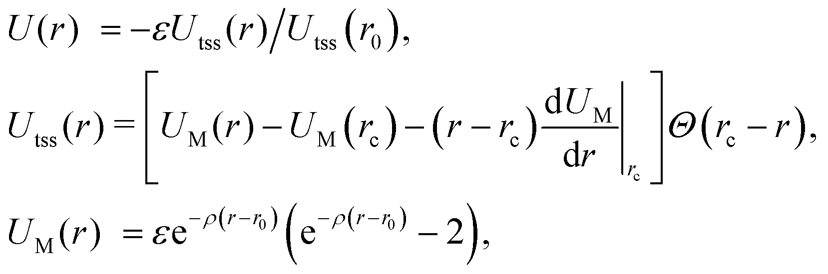where r is the separation of the two particles and r₀ is the equilibrium pair separation. These distances are measured along the Euclidean line that joins the particles in three-dimensional space, rather than along the geodesic on the two-dimensional surface, as shown in Fig. 1. The Heaviside step function Θ in eqn (1) truncates the potential at a distance r_c. For this work we have chosen to set r_c/r₀ = 2.23, in line with comparable investigations.^11,25 The potential is plotted in Fig. 1.

Fig. 1 Left: Toroidal surface, coloured by the local Gaussian curvature K in units of 1/r₀². The two size parameters a and c are labelled on the cross-section. The angles θ and ϕ specify the location of particles on the surface. Also depicted are two particles and the line through which the Morse potential acts. Note that the potential depends on the Euclidean distance marked r in three-dimensional space, rather than on the geodesic separation of the particles on the surface of the torus. Right: The truncated, shifted, smoothed and scaled Morse potential for some representative values of ρ.

2.2 Monte Carlo simulations

Canonical Monte Carlo (MC) simulations are used to survey the thermodynamic properties for a given number N of particles over a range of temperatures and values of ρ. The particle positions are specified in a system of two-dimensional curvilinear coordinates that are natural for the surface in question, such as the toroidal (ϕ) and poloidal (θ) angles of the torus in Fig. 1. Uniformly distributed trial displacements are made in the curvilinear coordinates of one particle per MC step, up to a fixed maximum size (chosen to achieve an acceptance rate of approximately 50%). Because of the nonlinearity of the coordinates, the Metrpolis acceptance criterion must be generalised to the formin order to achieve uniform sampling on the surface. In eqn (2), k_B is Boltzmann's constant and T is the temperature, U_n/o is the total potential energy of the displaced particle at its new/old position, and g_n/o is the square root of the determinant of the metric tensor at the new/old position. Explicit expressions for the g factors in terms of the relevant curvilinear coordinates will be stated when the surfaces are introduced.

To simulate a liquid phase covering the entire surface, we will need grand canonical MC, where N fluctuates in response to an imposed chemical potential μ. In practice,²⁶ the control parameter is the activity z(μ) = A₀Λ⁻² exp(μ/k_BT), where A₀ is the area of the surface and Λ is the thermal de Broglie wavelength. Working in terms of z avoids the need to specify Λ. In order to produce uniformly distributed trial positions for the particle-insertion moves, we generate random coordinates distributed according to the metric factor g by rejection sampling.²⁷

2.3 Molecular dynamics simulations

Molecular dynamics (MD) simulations will be used to observe transitions between different states on the phase diagram as a function of time. In these simulations, three-dimensional Cartesian coordinates are used and a one-body RATTLE-like constraint is applied to each particle. The algorithm forces the particles to remain on the surface and to have velocity vectors that lie in the local tangent plane of the surface.²⁸ We use the implementation by Paquay et al.²⁸ in the LAMMPS package.²⁹

For compatibility with the MC simulations, the MD simulations are performed at constant temperature using a Langevin thermostat. The damping time is set to 10 in the natural Morse time units of r₀(m/ε)^1/2, where m is the mass of one particle.

2.4 Global optimisation

We use basin-hopping with parallel tempering³⁰ (BHPT) in the GMIN program³¹ to search for ground-state structures, i.e., the globally lowest point on the potential energy landscape of a given system.

The basic basin-hopping algorithm³² is a MC simulation on the transformed potential energy surface

Ũ(X) = lmin[U(X)],

in which the energy Ũ assigned to a configuration X is that obtained by performing a local minimisation (lmin) of the true potential U starting from X. Hence, the potential energy surface is mapped onto a series of plateaux, each corresponding to the basin of attraction of a mechanically stable structure. This transformation removes the barriers between directly connected pairs of minima, thereby facilitating exploration of the surface and identification of the global minimum, whose energy is not affected.

Basin-hopping calculations can nevertheless become trapped in limited regions of the potential energy surface, especially if the surface is rough or contains multiple funnels. As in ordinary MC simulations, the efficiency of sampling can be enhanced with parallel tempering (also known as replica exchange).^33,34 In BHPT,³⁰ several basin-hopping replicas run in parallel at different temperatures, and trial moves occasionally attempt to exchange the configurations currently being sampled by two runs with adjacent temperatures. An exchange between replicas i and j with reciprocal temperatures β_i and β_j is accepted with probability

P^exch_ij = min[1,exp{−(β_i − β_j)(Ũ(X_i) − Ũ(X_j))}].

For BHPT on a torus, a single MC step involves displacing all particles by moving each one randomly onto a small sphere centred on its original position and then projecting back to the closest point on the torus. This procedure does not strictly preserve detailed balance, but this is not important since BHPT only attempts to locate the global potential energy minimum rather than to sample a thermodynamic ensemble. The advantage of these moves is that they produce roughly uniform displacements at all points on the torus, unlike steps of fixed maximum size in the toroidal and poloidal angles.

3 Results

3.1 Localised states on a torus

We have chosen a toroidal surface as our primary example of a surface with varying curvature for the following reasons: it is relatively simple, both mathematically and conceptually; it has regions of positive and negative Gaussian curvature; some progress is being made in reproducing it experimentally;^4,35,36 and related surfaces can be found in nature (for example the torovirus mentioned above²).

The toroidal case is governed by three independent length scales: the major radius c and the minor radius a of the torus, and the (inverse) range of the Morse potential ρ, all of which can be expressed in relation to the nominal particle diameter r₀ (see Fig. 1). The metric g factors appearing in eqn (2) are given by g = c + acos(θ), where θ is defined in Fig. 1. We focus on simulations carried out with N = 300 particles on a torus with a = 5r₀ and c = 7r₀, which we call a “5–7 torus”. This case illustrates all the general phenomena that we need to discuss. However, it is natural to ask how the detailed picture changes upon varying the number of particles or the geometry of the surface. In Section S3 of the ESI‡ we have therefore provided comparisons for smaller and larger values of N on the same torus, as well as for N = 300 on the thinner 3.5–10 torus.

Surface curvature can influence the free energy of a cluster on the surface in three ways:

(1) The length of the perimeter of a cluster of a given area depends on the underlying curvature, changing the line tension contribution to the free energy.¹⁷ In regions of positive Gaussian curvature, the perimeter is generally smaller than on a surface with zero or negative Gaussian curvature.

(2) A hexagonal crystal structure is necessarily distorted in regions of non-zero Gaussian curvature, leading to a stress that penalises the free energy.^11,12

(3) Curvature can make the interactions between next-nearest neighbours more favourable. For example, in a region of large negative Gaussian curvature (a saddle), the area immediately around a given particle increases more rapidly with distance on the curved surface than it would on a plane, allowing next-nearest neighbours to approach more closely. Furthermore, if the interactions act through space as they do in our model (rather than geodesically along the curved surface), any region with a large principal curvature will bring next-nearest neighbours closer in space. This latter effect can contribute even if the Gaussian curvature is zero (for example on cylinders and cones).

We will refer to the three contributions by the italicised terms above. The effects respond to curvature in different ways and they apply to the conventional states of matter (gas, liquid, solid) to different extents. The resulting couplings compete with each other to produce a rich set of stable states that are defined not only by the phase but also by the location of matter on the surface. We will denote the phase by a letter (G, L, C, X), and the location by the sign of the local Gaussian curvature (+, −, 0, ±). The meanings of the symbols are summarised in Table 1.

Table 1 Symbols used to denote the phase and location of thermodynamically stable states

Symbol	Meaning
G	Gas phase (covering whole surface)
L	Liquid phase
C	Condensed phase (intermediate order)
X	Crystal phase
+	Region of positive Gaussian curvature
−	Region of negative Gaussian curvature
0	Region of zero Gaussian curvature (and vicinity)
±	Spanning regions of negative and positive curvature

---

It is important to note that in any system with a small number of particles, phase transitions are somewhat smeared out. In particular, the onset of ordering in crystal-like states of our system is not sharp. Hence, Table 1 includes a condensed (C) phase within which the degree of crystallinity varies smoothly from liquid-like to crystal-like. We quantify the crystallinity by counting the number of particles N_X in a crystalline environment. To determine whether a given particle is crystalline, we select all particles within r = 1.45r₀ of it. These n neighbours are gnomonically projected onto the plane tangent to the surface at the target particle.³⁷ The magnitude of the bond-orientational order parameter is then calculated using

where θ_j is the angle between the target particle, the jth neighbour and some arbitrary local reference direction³⁸ (|ψ| does not depend on the choice of this direction). Particles with |ψ| > 0.6 are considered crystalline. It is important to note that this definition of |ψ| does not count particles on the edge of an ordered cluster as crystalline because of the missing neighbours.

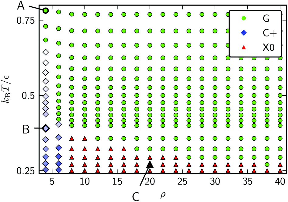
Canonical Monte Carlo simulations of 300 particles on the 5–7 torus reveal four stable states: G, L−, C+ and X0. Snapshots of these states are shown in Fig. 2 and their regions of thermodynamic stability are mapped out as a “phase diagram”' in the plane of temperature and potential range ρ in Fig. 3. We briefly survey the origin of these states before examining their coexistence and interconversion in Section 3.2, and analysing the competition between them in Section 3.3.

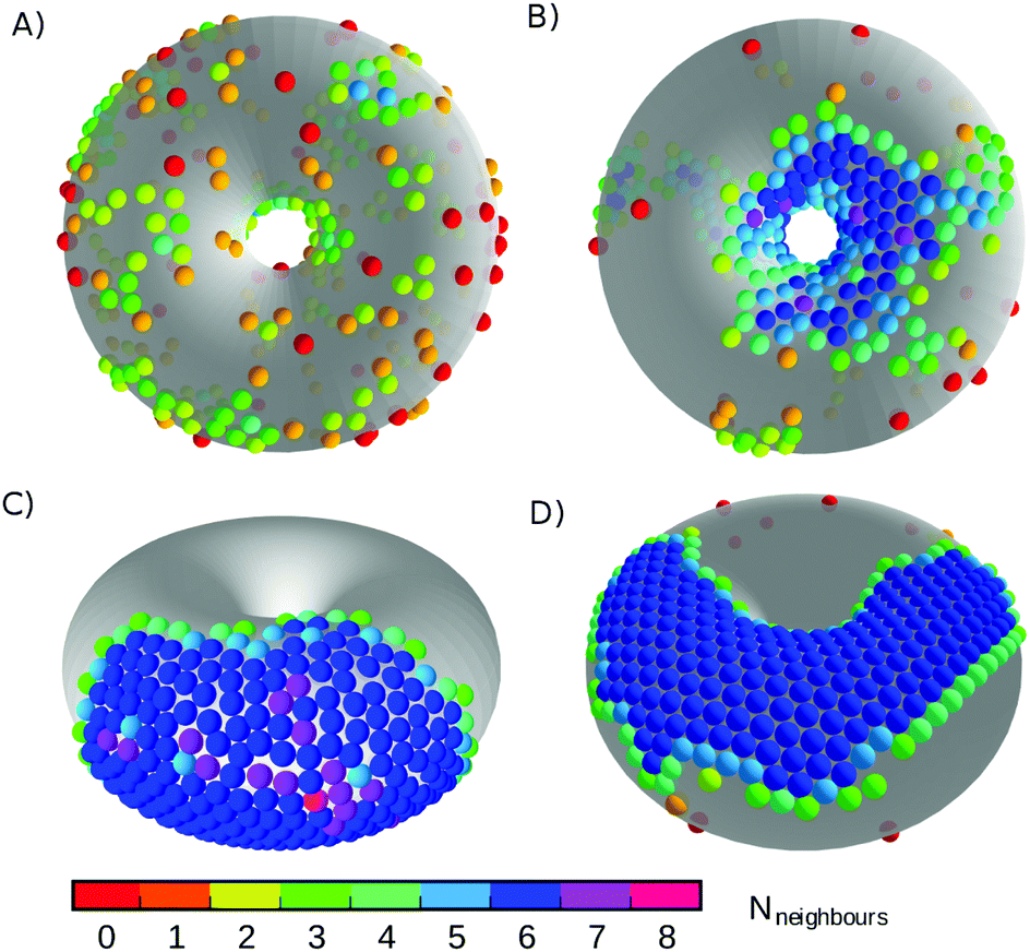Fig. 2 Snapshots of the states labelled in the phase diagram of Fig. 3. (A) G, at ρ = 6, k_BT/ε = 0.72; (B) L−, at ρ = 6, k_BT/ε = 0.42; (C) C+, at ρ = 4, k_BT/ε = 0.32; and (D) X0, at ρ = 18, k_BT/ε = 0.27. Particles are coloured by the number of nearest neighbours. The states are named according to the convention in Table 1.

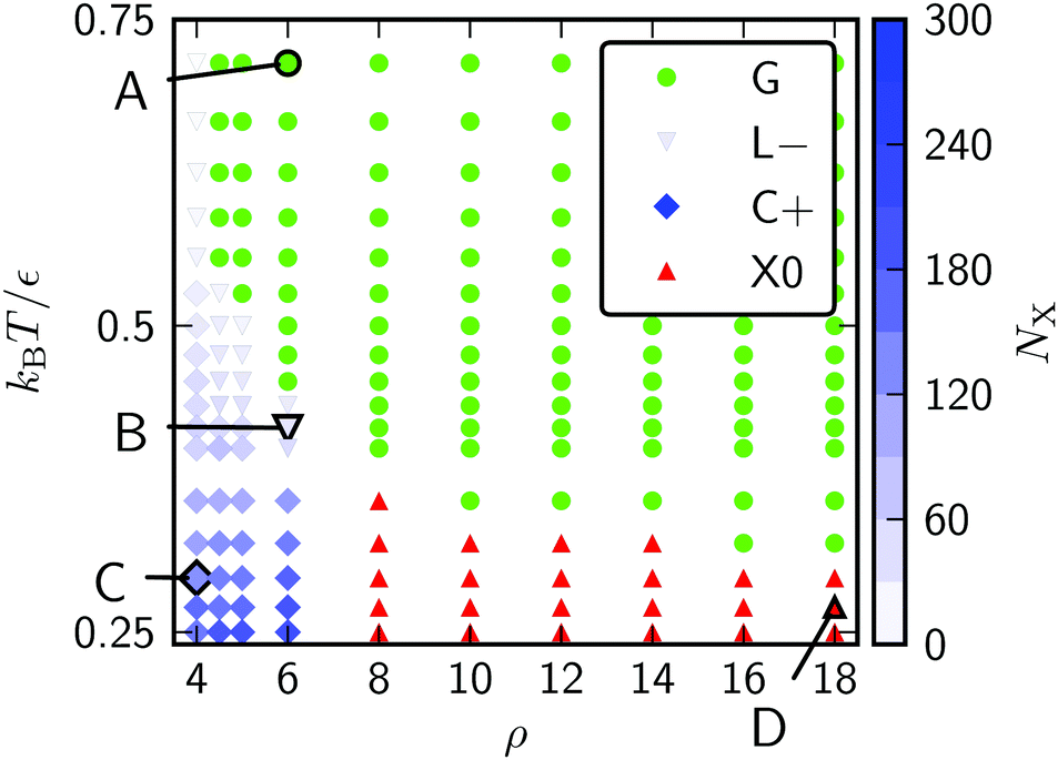Fig. 3 Phase diagram for 300 Morse particles on a 5–7 torus. The saturation of the blue symbols represents the crystallinity, showing a steady increase as the C+ state is cooled. Snapshots of the points labelled A–D are given in Fig. 2.

As expected, the particles cover the torus in a low-density gas-like state G at sufficiently high temperature for any range of the potential. Lowering the temperature at long range (ρ ≤ 6) leads to a gas–liquid transition. In the liquid state, the neighbour effect (described above) is strong enough to drive the cluster to the centre of the torus, where the mean curvature is largest. The Gaussian curvature in that region is negative, so this localised state is denoted L−. Reducing the temperature further produces a driving force towards crystalline order, but regions of high Gaussian curvature are incompatible with regular hexagonal packing and the stress effect becomes increasingly important. The cluster therefore moves to a C+ state on the outside of the torus, where the mean curvature is lower (thereby relieving some stress) but where it can still adopt a compact shape to reduce its perimeter. We measure the order in the C+ state by the number N_X of crystalline particles, i.e., the number of particles with |ψ| > 0.6. Plots and a discussion of the distribution of |ψ| itself can be found in ESI,‡ Section S2. Defined this way, the structure within the C+ state varies smoothly between liquid and crystalline, as indicated by the intensity of the shading in Fig. 3 However, the C+ state is separated from the neighbouring L− and X0 states by decisive shifts in location of the cluster. In Section 3.2 we will confirm that the C+ state is a distinct free-energy minimum.

Moving at constant temperature to shorter-ranged potentials (horizontally to the right in Fig. 3), another transition is reached. Deviations from perfect hexagonal packing become more energetically costly because of the increasing second derivative at the minimum of the potential well (Fig. 1), and the stress effect starts to dominate over the perimeter effect. As a result, a crystal state, X0, forms as a ribbon on the top (or bottom) of the torus, where the Gaussian curvature, and therefore the stress, is lowest. This highly elongated structure comes at the expense of a long perimeter. Heating this crystal causes it to sublime directly back to the G state.

As a reference system without the effects of curvature, we may compare a square plane of edge 37.17r₀ with the same area as the 5–7 torus but with conventional periodic boundary conditions. The phase diagram for 300 Morse particles on the plane contains the three standard phases G, L and X and is given in Fig. S5 (ESI‡). Apart from the absence of location specifiers, the phase diagram is similar to that in Fig. 3. The new C+ condensed state on the torus mostly occupies regions that would be crystalline (X) on the plane where the potential is soft enough for some stress to be accommodated in return for a shorter perimeter. Relative to the planar system, curvature also moves the gas–liquid boundary slightly in favour of the liquid, due to the additional liquid stability that comes from the neighbour effect in the presence of curvature.

Both the toroidal and planar systems lose their liquid phases at high ρ. This happens for the same reasons as in three-dimensional systems; a decrease in the range of the potential causes the gap between the triple point and the gas–liquid critical point to grow narrower until the gap vanishes altogether, leaving no temperature at which the liquid is thermodynamically stable.³⁹

As an example of a torus with a different aspect ratio, we have also studied the torus with a = 3.5r₀ and c = 10r₀, which has the same surface area as the 5–7 torus. The thinner tube and wider bore of the 3.5–10 torus introduce a liquid-like state that is stabilised by wrapping round the tube to reduce the perimeter. A more detailed treatment of this case, including the phase diagram, is provided in ESI,‡ Section S3D.

3.2 Free energy surfaces and dynamics

Returning to the main case of the 5–7 torus, a direct implication of the phase diagram in Fig. 3 is that each of the localised states is the global free energy minimum for a range of T and ρ. At the boundaries between states, we expect pairs of free energy minima to coexist and to be separated by a barrier. Because of the coupling of phase and location, the pathways between free energy minima must involve migration of matter on the toroidal surface.

To visualise the free energy and trajectories, we project onto the plane of two order parameters. To track the phase, one of the order parameters is the number N_X of crystalline particles, as defined in Section 3.1. To track location, the second order parameter is the density n₊ of particles in a region of positive Gaussian curvature (the “outside” of the torus in Fig. 1), as a fraction of the total density n: n₊/n. The free energy surface is now constructed by accumulating a two-dimensional histogram H of the order parameters during a canonical MC simulation and taking F = −k_BT ln H. As we shall see, the barriers on this surface are sufficiently low that no special sampling techniques are needed to obtain good statistics.

In Fig. 4, we present the free energy surface at three different points on the phase diagram. Each point lies close to a phase transition and shows two minima, indicating that two states coexist. Fig. 4(A) is taken close to the transition between the L− and C+ states. The transition involves both a dramatic shift of particles towards the outside of the torus and a slight increase in crystallinity (although at this temperature, the C+ phase is still liquid-like, see Fig. 3).

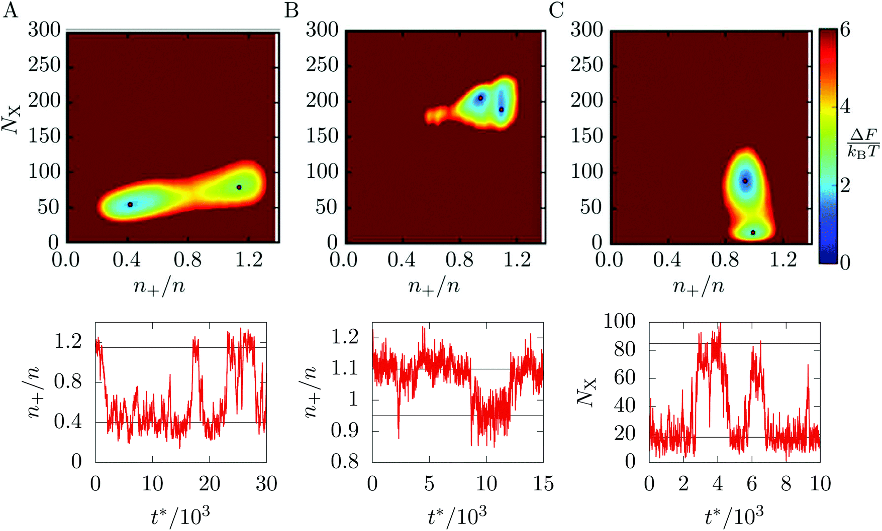Fig. 4 Upper panels: free energy surfaces for 300 Morse particles on a 5–7 torus with minima highlighted by red dots. (A) At ρ = 6 and k_BT/ε = 0.39. The red dots indicate the L− (left) and C+ (right) states. (B) At ρ = 7 and k_BT/ε = 0.25. The red dots indicate the X0 (left) and C+ (right) states. (C) At ρ = 20 and k_BT/ε = 0.30. The red dots indicate the G (bottom) and X0 (top) states. Lower panels: samples of the corresponding dynamic trajectories switching between the free energy minima, with horizontal lines denoting the minima. Time is measured in reduced units , where t is the real time and m is the mass of a particle.

Fig. 4(B) shows the vicinity of the transition from the C+ state to the X0 state. As the temperature here is lower, the C+ phase is more crystalline and therefore appears further along the vertical axis of the free energy plot than in panel (a). The evolution of the minimum on the free energy surface with temperature is smooth and does not involve any barriers, justifying our treatment of C+ as a single phase of intermediate crystalline character. The figure shows that the transition from C+ to X0 is accompanied by a slight increase in crystallinity and a shift of particles away from the outside of the torus.

The last panel, Fig. 4(C) shows the coexistence between the G and X0 states, which mainly involves a change in crystallinity as both states are distributed fairly evenly between the inside and outside of the toroidal surface.

Having identified these coexisting pairs of states, we then used surface-constrained molecular dynamics simulations to observe the bulk translation of the clusters as the system switched back and forth between the states. For each free energy surface in Fig. 4, we performed a single simulation at fixed temperature and ρ and monitored the order parameter most relevant to the transition in question. The plot below each free energy map shows part of the resulting equilibrium time trace of the order parameter. In each case, the trace shows rapid switches of the system between two states, with comparatively long residence times within the states, confirming the interpretation of the distinct macrostates identified in Section 3.1. In the ESI‡ we have included videos that visualise an example pathway for each of the three transitions.

3.3 The competing effects of curvature

In this section, we provide a more quantitative analysis of the three effects of curvature identified in Section 3.1. The results provide insight into the competition between the effects and the factors that influence the points where they balance. In turn, this helps to generalise the principles to other examples of non-uniformly curved two-dimensional systems.

For liquid-like states, the optimal location is determined by the perimeter and neighbour effects. On the torus, these two effects compete with each other because the most strongly curved region (beneficial for next-nearest neighbours) is on the inside of the torus, but the sign of the Gaussian curvature is negative there, so the perimeter is larger for a given area (costing line energy). We have obtained the optimal perimeters as a function of the enclosed area using constrained minimisation in the Surface Evolver software.⁴⁰ By carefully choosing the symmetry of the initial patch about poloidal angles θ = 0 and 180°, the optimisation can be performed separately for patches in the regions of positive and negative curvature, respectively. The two perimeters are plotted in Fig. 5(A), showing the increasing advantage of the C+ state with area.

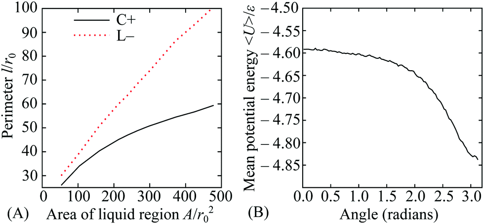Fig. 5 (A) Minimised perimeter of the liquid–gas interface for the C+ and L− states as a function of the area of the liquid region. (B) Average potential energy per particle in a surface-covering liquid state as a function of the poloidal angle θ, taken from a grand canonical simulation at ρ = 6, k_BT/ε = 0.48 and activity z= 57.544.

The contribution of the potential energy to the neighbour effect can also be quantified by examining the mean energy per particle as a function of the poloidal angle θ in a liquid that covers the whole surface. We have obtained a specimen system-covering fluid by performing a grand canonical simulation of particles with range parameter ρ = 6 at a temperature of k_BT/ε = 0.48 and activity z = 57.544. The location dependence of the mean potential energy is shown in Fig. 5(B), where it can be seen that the energy per particle is some 5% lower on the inside of the torus than on the outside.

The plots in Fig. 5 demonstrate two of the key ingredients in the perimeter and the neighbour effects. Other important considerations include the line tension on the perimeter itself, which is much harder to evaluate. However, the full complexity of the resulting competition between the C+ and L− states can be seen by tracking the relative depths of the corresponding free energy minima in Fig. 4(A) as a function of the total number N of particles in the system. For potential range ρ = 6 and temperature k_BT/ε = 0.37, the two states coexist as (meta)stable minima at least from N = 100 to 300 and their relative free energies are shown over this range in Fig. 6. Interestingly, the lines cross twice, emphasising the nonlinearity of the perimeter and neighbour effects with respect to N.

Fig. 6 Depth of the free energy minima of the L− and C+ states on the 5–7 torus for ρ = 6 at reduced temperature k_BT/ε = 0.37. The origin of the vertical scale is arbitrary; only comparisons between the two lines matter.

The phase diagram in Fig. 3 shows that there is a competition between the C+ and X0 states as a function of the potential range parameter ρ at low temperature. Under these conditions, the potential energy is the dominant contribution to the free energy and it is instructive to locate the global potential energy minima using BHPT. The optimisation runs used eight parallel replicas with an exponential distribution of temperatures in the range 0.3 ≤ k_BT/ε ≤ 2 and up to 60 000 basin-hopping steps per case. Runs were initiated with quenched structures from canonical MC simulations. Fig. 7 shows the resulting putative global minima for a soft (ρ = 4) and a stiff (ρ = 18) interaction potential for our case study of N = 300, while sequences of global minima from N = 100 to 500 are presented in Section S1A of the ESI.‡ To highlight any packing defects in these structures, we have depicted them by their Voronoi tesselations. To avoid ill-defined Voronoi cells at the edges of the clusters, any Voronoi vertex lying further than 1.3r₀ from its particle has been deleted in the analysis, and any Voronoi cell with fewer than five edges is not displayed in the figure. These measures have the effect of discarding most cells corresponding to edge particles but they do not alter the depiction of the cluster interiors.

Fig. 7 Putative global potential energy minimum structures for N = 300 particles on the 5–7 torus for (A) range parameter ρ = 4 (C+ configuration), (B) ρ = 18 (X0). The structures are depicted by their Voronoi tessellations and the colour of each cell corresponds to the coordination number of the particle that it contains (colour scheme as in Fig. 2). (C) Potential energy of the C+ and X0 minima as a function of the range parameter ρ for N = 300 particles on the 5–7 torus.

The long-ranged potential is able to accommodate the stress on the hexagonal lattice in the region of positive Gaussian curvature on the outside of the torus, characteristic of the C+ thermodynamic state [Fig. 7(A)]. This stress is manifest mostly as a systematic and delocalised distortion of the packing, but a packing defect is also visible in the centre of the cluster. The defect consists of three pentagonal tiles and two heptagonal tiles, giving a positive overall topological charge of +1, as expected in a region of positive Gaussian curvature.⁴¹ Such defects are too costly for short-ranged potentials because a lower formal coordination number involves losing most (not just some) of the interaction with a neighbouring particle. Even delocalised stress is highly unfavourable because of the sensitivity of the potential near its minimum. Hence, the global minimum changes to lie in the flattest region of the surface like the X0 thermodynamic state [Fig. 7(B)]. The cluster is now far less compact and the increase in its perimeter, demarcated by low-coordination particles, is readily visible.

We can estimate the point at which the X0 state takes over from C+ by tracking the energy of the two structures depicted in Fig. 7 as a function of ρ. We do this by incremental changes in ρ, each followed by a local minimisation to relax the structure to the point of mechanical equilibrium without significant rearrangement. Both structures persist as (meta)stable minima over a wide range of ρ. The resulting potential energy curves are compared in Fig. 7(C), showing that they cross at ρ ≈ 8, which is consistent with the boundary between C+ and X0 in the finite-temperature phase diagram of Fig. 3. Further insight can be gained from the comparison in Fig. 7(C) by decomposing the energy into contributions with a direct physical interpretation. This analysis is provided in Section S1B of the ESI.‡

The competition between the perimeter, stress and neighbour effects is altered by the scale, as well as by the shape, of the surface. Any given torus has a finite surface area and – like a sphere – can only accommodate a limited number of particles before overcrowding incurs a steep free energy penalty.¹⁸ However, consider a thought experiment in which the two radii a and c of the torus are both increased by a factor f, keeping the aspect ratio fixed, and the number of particles N is increased by f² to keep the surface coverage approximately equal. This scaling would uniformly reduce the Gaussian curvature by a factor of 1/f². Hence, the neighbour effect, which relies on local curvature, would become less important with increasing f, and this is likely to destabilise the L− state. However, the perimeter would increase approximately as f (for a given cluster shape) and, for states with crystalline character, there would also be an increase in stress.¹² As we have seen (for example, in Fig. 7), stress introduces a complex interplay between elastic energy and defects, the energetic cost of which depends on the interaction potential. Hence, we can expect a non-trivial evolution of structure and stability with overall scale of the host surface, even at fixed aspect ratio.

3.4 A sinusoidal surface

To demonstrate that the phenomena seen on the torus can be extended to other curved surfaces, we have performed simulations on a sinusoidal surface with periodic boundaries, defined in Cartesian coordinates x, y, z by

z = h sin(2πx/L)sin(2πy/L).

We set h = 7.5r₀ and L = 30.75r₀ so that the area and maximum Gaussian curvature of this surface match those of the 5–7 torus. The metric g factors for use in eqn (2) are now given by

Snapshots of the stable states of this system are presented in Fig. 8 and the phase diagram is shown in Fig. 9. This system has only three states: G, C+ and X0. At high temperature, the system is found in the G state. For softer (longer-ranged) potentials, as the system is cooled the particles condense into a liquid phase, C+, which is always found on one of the peaks or troughs of the surface. This configuration is preferred both for its short perimeter and for its high mean curvature (leading to a favourable neighbour effect). As the system is cooled further, the condensed cluster becomes more crystalline. Although the contribution of stress in the crystal to the free energy is increasing, at low ρ the cluster does not move again, unlike on the torus which has the transition from L− to C+. We suggest that this is because the line tension is high enough that, unlike on the torus, moving to a less curved region with a longer perimeter would not be favourable. However, at higher values of ρ, the system crystallises around the flanks of the peaks, where the Gaussian curvature is lowest, giving an X0 state. As in the corresponding X0 state on the torus, as well as in the branched structures observed by Meng et al.¹² on spherical droplets, a longer perimeter is traded for less frustration in stiffer crystals.

Fig. 8 Snapshots of states for 300 particles on a periodic sinusoidal surface. (A) G, at ρ = 4, k_BT/ε = 0.78; (B) C+, at ρ = 4, k_BT/ε = 0.39; and (C) X0, at ρ = 20, k_BT/ε = 0.27. Particles are coloured by the number of nearest neighbours (see Fig. 2 for key).

Fig. 9 Phase diagram for 300 Morse particles on a periodic sinusoidal surface as a function of the potential range parameter ρ and the reduced temperature k_BT/ε. Snapshots of the points labeled A–C are given in Fig. 8.

An important message from comparing the torus and the sinusoidal surface is that the relationship between the perimeter, stress and neighbour effects is determined by the shape of the surface. For example, the regions of largest principal curvature on the sinusoidal surface are the peaks and troughs, where the Gaussian curvature is positive. Hence, the perimeter and neighbour effects reinforce each other in this region. In contrast, the largest principal curvature on a torus is around the central bore, where the Gaussian curvature is negative, leading to antagonism between the perimeter and neighbour effects. Nevertheless, it is the same set of physical arguments that comes into play in all cases.

4 Conclusions

We have shown that, in non-uniformly curved two-dimensional systems, clusters of attractive colloids minimise their free energy by adopting specific shapes and translating to specific locations. The equilibrium shape and location depends not only on the phase of matter in the cluster, but also on the range of the interaction potential and the curvature of the underlying surface. The coupling of phase to shape and location leads to dramatic reorganisation of matter as the conditions are varied. In particular, phase transitions can be accompanied by wholesale migration of matter to different parts of the surface. We have demonstrated that these effects arise in systems where the particles themselves are simple spheres with isotropic interactions. These particles collectively respond to curvature despite having no individual preference for a particular curvature or a curvature-adapted shape.

We have identified three universal contributions to the free energy that drive the behaviour: the length of the cluster perimeter, the stress on packing induced by Gaussian curvature, and the distances from a given particle to its next-nearest neighbours. These considerations explain the four phase-location coupled states that we observe on a torus and the three states on a sinusoidal surface. Free energy calculations also showed the barriers between these states and molecular dynamics simulations confirmed the switching between them.

There are a number of avenues for future investigations in which the phase behaviour is strongly affected by non-uniform curvature. For instance, we expect additional levels of control and rich behaviour in cases where surface curvature is coupled with an anisotropic interaction potential or polydisperse mixtures. It would also be interesting to analyse in detail the defects observed in the C+ and X0 states, at both zero and finite temperature, and in particular to study whether they follow existing predictions on how the number of defects depends on the amount of curvature enclosed^41,42 and the effects of thermal fluctuations.⁴³ Another open question is the case where the confining surface is flexible, where the curvature responds to the particles that are confined upon it. This latter form of coupling is relevant, for example, in a variety of clustering and aggregation phenomena on lipid membranes.¹

We hope our work will motivate experimental demonstrations of the cooperative curvature-sensing effects shown in this article, in both biological and engineered systems. Due to the generality of the effects, the non-uniformly curved surface need not be specifically toroidal or sinusoidal as in the examples presented here.

Conflicts of interest

There are no conflicts to declare.

Acknowledgements

The authors thank Stefan Paquay for advice on the MD simulations. J. O. L. is grateful to the Engineering and Physical Sciences Research Council (EPSRC) Centre for Doctoral Training in Soft Matter and Functional Interfaces (SOFI, grant EP/L015536/1) for financial support.

Notes and references

1. A. Vahid, A. Saric and T. Idema, Soft Matter, 2017, 13, 4924–4930.
2. L. Giomi and M. J. Bowick, Phys. Rev. E: Stat., Nonlinear, Soft Matter Phys., 2008, 78, 010601.
3. F. Paillusson, M. R. Pennington and H. Kusumaatmaja, Phys. Rev. Lett., 2016, 117, 058101.
4. P. W. Ellis, D. J. G. Pearce, Y.-W. Chang, G. Goldsztein, L. Giomi and A. Fernandez-Nieves, Nat. Phys., 2017, 14, 85–90.
5. Q. Liu, B. Senyuk, M. Tasinkevych and I. I. Smalyukh, Proc. Natl. Acad. Sci. U. S. A., 2013, 110, 9231–9236.
6. I. B. Liu, G. Bigazzi, N. Sharifi-Mood, L. Yao and K. J. Stebe, Phys. Rev. Fluids, 2017, 2, 100501.
7. T. Rehman and V. N. Manoharan, personal communication, 2018.
8. N. D. Bade, T. Xu, R. D. Kamien, R. K. Assoian and K. J. Stebe, Biophys. J., 2018, 114, 1467–1476.
9. F. C. Keber, E. Loiseau, T. Sanchez, S. J. DeCamp, L. Giomi, M. J. Bowick, M. C. Marchetti, Z. Dogic and A. R. Bausch, Science, 2014, 345, 1135–1139.
10. T. Lopez-Leon, V. Koning, K. B. S. Devaiah, V. Vitelli and A. Fernandez-Nieves, Nat. Phys., 2011, 7, 390–394.
11. S. Paquay, G.-J. Both and P. van der Schoot, Phys. Rev. E, 2017, 96, 012611.
12. G. Meng, J. Paulose, D. R. Nelson and V. N. Manoharan, Science, 2014, 343, 634–637.
13. D. Joshi, D. Bargteil, A. Caciagli, J. Burelbach, Z. Xing, A. S. Nunes, D. E. P. Pinto, N. A. M. Araújo, J. Brujic and E. Eiser, Sci. Adv., 2016, 2, e1600881.
14. F. L. Jiménez, N. Stoop, R. Lagrange, J. Dunkel and P. M. Reis, Phys. Rev. Lett., 2016, 116, 104301.
15. A. R. Bausch, M. J. Bowick, A. Cacciuto, A. D. Dinsmore, M. F. Hsu, D. R. Nelson, M. G. Nikolaides, A. Travesset and D. A. Weitz, Science, 2003, 299, 1716–1718.
16. Z. Yao, Soft Matter, 2017, 13, 5905–5910.
17. L. R. Gómez, N. A. Garca, V. Vitelli, J. Lorenzana and D. A. Vega, Nat. Commun., 2015, 6, 6856–6865.
18. J. O. Law, A. G. Wong, H. Kusumaatmaja and M. A. Miller, Mol. Phys., 2018, 116, 3008–3019.
19. D. Marenduzzo and E. Orlandini, Soft Matter, 2012, 9, 1178–1187.
20. V. Vitelli, L. B. Lucks and D. R. Nelson, Proc. Natl. Acad. Sci. U. S. A., 2006, 103, 12312–12328.
21. H. Kusumaatmaja and D. J. Wales, Phys. Rev. Lett., 2013, 110, 165502.
22. W. T. M. Irvine, V. Vitelli and P. M. Chaikin, Nature, 2010, 468, 947–951.
23. H. T. McMahon and J. L. Gallop, Nature, 2005, 438, 590–596.
24. B. Antonny, Annu. Rev. Biochem., 2011, 80, 101–123.
25. J.-P. Vest, G. Tarjus and P. Viot, Mol. Phys., 2014, 112, 1330–1335.
26. D. Frenkel and B. Smit, Understanding Molecular Simulation, Academic Press, San Diego, 2nd edn, 2002.
27. L. Martino and J. Mguez, Signal Process., 2010, 90, 2981–2995.
28. S. Paquay and R. Kusters, Biophys. J., 2016, 110, 1226–1233.
29. S. Plimpton, J. Comput. Phys., 1995, 117, 1–19.
30. B. Strodel, J. W. L. Lee, C. S. Whittleston and D. J. Wales, J. Am. Chem. Soc., 2010, 132, 13300–13312.
31. D. J. Wales, GMIN: A program for finding global minima and calculating thermodynamic properties from basin-sampling, http://www-wales.ch.cam.ac.uk/GMIN.
32. D. J. Wales and J. P. K. Doye, J. Phys. Chem. A, 1997, 101, 5111–5116.
33. A. P. Lyubartsev, A. A. Martsinovski, S. V. Shevkunov and P. N. Vorontsov-Velyaminov, J. Chem. Phys., 1992, 96, 1776–1783.
34. C. J. Geyer and E. A. Thompson, J. Am. Stat. Assoc., 1995, 90, 909–920.
35. J.-K. Kim, E. Lee, Z. Huang and M. Lee, J. Am. Chem. Soc., 2006, 128, 14022–14023.
36. V. Haridas, A. R. Sapala and J. P. Jasinski, Chem. Commun., 2015, 51, 6905–6908.
37. J. P. Snyder, Map projections: A working manual, USGS publications warehouse technical report, 1987.
38. B. I. Halperin and D. R. Nelson, Phys. Rev. Lett., 1978, 41, 121–124.
39. M. H. J. Hagen and D. Frenkel, J. Chem. Phys., 1994, 101, 4093–4097.
40. K. A. Brakke, Exp. Math., 1992, 1, 141–165.
41. C. J. Burke, B. L. Mbanga, Z. Wei, P. T. Spicer and T. J. Atherton, Soft Matter, 2015, 11, 5872–5882.
42. S. Li, R. Zandi, A. Travesset and G. M. Grason, Phys. Rev. Lett., 2019, 123, 145501.
43. S. Paquay, H. Kusumaatmaja, D. J. Wales, R. Zandi and P. van der Schoot, Soft Matter, 2016, 12, 5708–5717.

---

Footnotes

† An archive of raw data and code is available at DOI: 10.15128/r1wh246s13w.

‡ Electronic supplementary information (ESI) available. See DOI: 10.1039/d0sm00652a

§ Present address: Department of Chemistry, University of Bath, Claverton Down, Bath BA2 7AY, UK.

---