Crossover from mean-field compression to collective phenomena in low-density foam-formed fiber material

Abstract

We study the compression of low-weight foam-formed materials made out of wood fibers. Initially the stress–strain behavior follows mean-field like response, related to the buckling of fiber segments as dictated by the random three-dimensional geometry. Our Acoustic Emission (AE) measurements correlate with the predicted number of segment bucklings for increasing strain. However, the experiments reveal a transition to collective phenomena as the strain increases sufficiently. This is also seen in the gradual failure of the theory to account for the stress–strain curves. The collective avalanches exhibit scale-free features both as regards the AE energy distribution and the AE waiting time distributions with both exponents having values close to 2. In cyclic compression tests, significant increases in the accumulated acoustic energy are found only when the compression exceeds the displacement of the previous cycle, which further confirms other sources of acoustic events than fiber bending.

---

1 Introduction

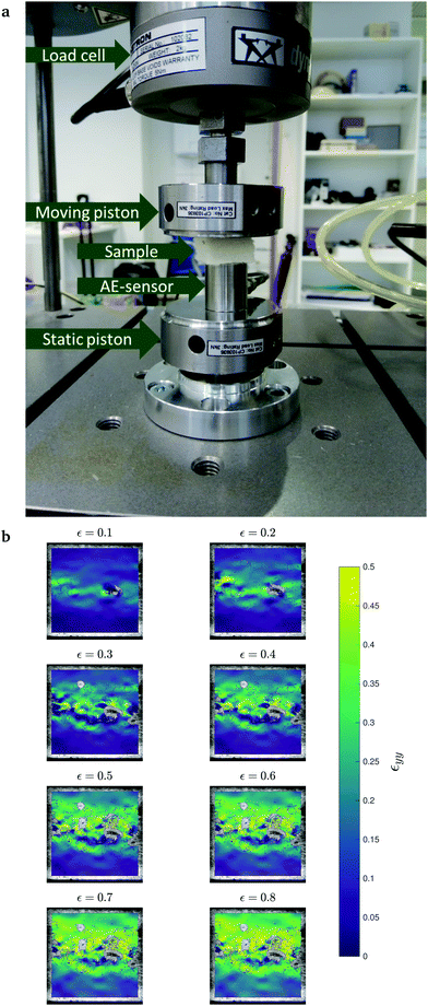
Soft, bio-based materials offer a wide range of material combinations and likewise a wide range of methods for synthesizing such. Networks based on fibers with high aspect ratio form as such a class of interesting examples. In particular, one interesting route is using aqueous foams to set up the fiber network geometry,^1–5 whereby the air bubbles of the carrier foam determine to a large degree the porous structure of the “fiber foam” after drying.⁶

The mechanics of random fiber networks depend first and foremost on the network density, or likewise on the number of contacts per fiber.⁷ Beyond that, the mechanical properties of the individual fibers and their variation play an important role,⁸ as does often the nature of the fiber-to-fiber bonds,⁹ in particular the character of the stress transfer and the bond failure mechanism. In what follows we study (see Fig. 1) the compression deformation of low-weight foam-formed wood fiber structures, in the density of 60 kg m⁻³. These structures have a random structure typically, and a low number of contacts per fiber. Using geometric arguments,^7,8 the average contact number would be 5–7 for homogeneous fiber distribution. However, the true number of inter-fiber bonds is probably somewhat higher because of voids and large pores left in samples after foam forming.

Fig. 1 (a) The experimental setup consists of Instron E1000 tensile testing machine that compresses the sample between two steel pistons and measures the applied force F. The acoustic emission is captured by a sensor below the sample. (b) The yy-component of the Green–Lagrange strain calculated by Digital Image Correlation for a CTMP sample at different strains. The deformation to around 10% strain shows strain concentration to the middle layer of the sample but this evens out after the initial compression.

Earlier simulations¹⁰ have shown the build up of significant axial stress in non-bonded fiber networks at high compaction levels. The axial stress should develop more rapidly in well-bonded networks with high fiber bending stiffness. Besides normal bending¹¹ and bond opening, possible local stress release mechanisms in this case are also the sudden buckling of the whole fiber segment or a localized buckling failure e.g. in the heterogeneous fiber wall of a hollow wood fiber. The latter could take place also in the case of fiber bending, where axial stress outside the neutral plane can be high. Ketoja et al.⁸ postulated that the mean stress–strain behavior during compression could be related to buckling failures of fiber segments. Effectively fiber segments that undergo a buckling failure would act as “stress sensors” that relate mean geometrical changes of the network with the applied stress. The postulate allows to solve for the stress–strain response using simple mean-field arguments to account for the gradually increasing fraction of fiber segments that have buckled.

In this work, we study what happens beyond the validity of such theory, at large compressional strains, while also providing further evidence for the mean-field argument at small strains. A large literature has grown recently around the presence of complex, collective phenomena in deformation under compression.^12–26 The main idea is the presence of “labquakes” or bursts of deformation analogous in many ways to earthquakes. Stress–strain curves and concomitant Acoustic Emission (AE) and digital image correlation analyses allow to characterize the burstiness and classify materials according to the statistics observed. The purpose of our work is to both explore the avalanches during the deformation of the foam-formed fiber structures and to relate the changes in stress–strain curves from mean-field-like behavior to the AE activity.

The next section discusses the experimental details, and then we in section Results show for two kinds of foam-formed fiber structures what kind of stress–strain behavior is found and what kind of AE statistics are obtained. Finally, we present conclusions and ideas for further study.

2 Experimental

The experimental setup is depicted in Fig. 1a where the foam-formed block of 19 × 20 × 20 mm³ is compressed between a compression piston and an AE sensor ensuring a good acoustic coupling. To obtain uniform compression a thin plastic plate wider than the sample was placed between the sample and the AE sensor. The AE sensor is a wideband sensor F30α connected to a preamplifier by Physical Acoustics Corporation. The steel and ceramic casing of the sensors is rigid within measurements accuracy under the small loads during the compression. The amplified signal is then digitized by National Instruments 6040E digital acquisition card with f = 100 kHz sample rate. The compressive piston is connected to a load cell with nominal maximum load of 250 N with 1% repeatability. The cell is connected to the Instron E1000 tensile testing machine that digitizes the load displacement data in compliance with the ASTM standards.

Additionally one face of the sample was imaged for Digital Image Correlation analysis. The Fig. 1b shows some typical compressive strain maps obtained using this method. The plotted ε_yy is the yy-component (where y is the compression direction) of the Green–Lagrange strain tensor obtained with the ncorr²⁷ software. The displacement calculations were done using circular regions of interest with radius of 25 pixels and grid spacing of 1 pixel which correspond to 0.75 mm and 0.03 mm. The component of the strain tensor considered is then calculated from the displacements u = (u,v) as

The missing parts in the maps are due to the inability of Digital Image Correlation to follow the extremely large strains. Interestingly, these maps indicate that the heterogeneity of the strain is relatively largest at the very beginning of the experiment. This indicates large local variations in the compressional modulus, which get smoothened out at larger strains.

2.1 Sample preparation

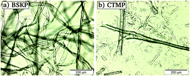
Two types of fiber materials were used to prepare the foam-formed samples: unrefined bleached softwood kraft pulp (BSKP) and bleached spruce chemi-thermomechanical pulp (CTMP) (see Fig. 2). BSKP was obtained from a Finnish pulp mill (Metsä Fibre Oy, Äänekoski Bioproduct Mill, Finland) with the Schopper–Riegler (SR) freeness value of 13, and CTMP was gained from a Swedish pulp mill (Rottneros AB, Rottneros Mill, Sweden) with the Canadian Standard Freeness value of 650. Both freeness values describe dewaterability of pulp and indirectly indicate fiber flexibility and fines content. The average (length-weighted) fiber length was 1.98 ± 0.02 mm for BSKP and 1.86 ± 0.03 mm for CTMP. The mean fiber widths were 28.3 ± 0.1 μm (BSKP) and 38.2 ± 0.2 μm (CTMP). However, the CTMP pulp included a much higher proportion of submicron fine particles than the BSKP pulp.

Fig. 2 Microscopic images of the two fiber types. The fibers in (a) bleached softwood kraft pulp (BKSP) appear more curved and flexible than the (b) chemi-thermomechanical pulp (CTMP) fibers that appear more stick-like.

In sample preparation, a nonionic surfactant polyethylene sorbitan monolaurate (TWEEN 20, Sigma-Aldrich, St. Louis, MO, USA) with the dosage of 6.5 g l⁻¹ was used as foaming agent. The high surfactant concentration, exceeding the critical micelle concentration of 0.074 g l⁻¹,²⁸ was necessary to achieve the target air content of wet foam. The wet fiber foams were generated by mixing the pulp, surfactant and water in a vessel with a starting volume of 3.08 liters, with a mixer (Netzsch, Hedensted, Denmark). A rotational speed of 3800 rpm was used to make the foam at the air content of 58%. After foaming, the wet foam was poured into a hand-sheet mold along a tilted plate and was left to drain for about 20 min by gravity. The sheets were dried over night at 70 °C in an oven. The final targeted thickness level was adjusted in a separate phase. The dried sheets were firstly re-wetted to a 50% moisture content and then pressed to the desired thickness (20 mm) and finally dried in an oven (70 °C). This resulted in porous random fiber networks with broad pore size distributions. Basis weights of the sheets were about 1200 g m⁻². Density of the CTMP and BSKP sheets were 60.6 and 63.6 kg m⁻³, respectively. For the experiments, blocks of the size of 20 × 20 mm² were cut from the sheets.

2.2 Acoustic emission

The observed acoustic emission signal A is divided into discrete events by thresholding it just above the noise level. The energy of each event is then calculated as the square integral of the amplitude over the event durationThe energy is therefore in arbitrary units but as the amplification and the sensor placement are kept the same, the energies are equivalent for all experiments. The occurrence time of the event t_i is defined as the time of the maximum amplitude and the waiting times are obtained as the time difference between successive events τ_i = t_i − t_i−1.

The event count n denotes the cumulative number of acoustic events and similarly the cumulative energy is the sum of the energies of the acoustic events. Similarly the event rate ṅ and the energy rate Ė_AE at time t are calculated by counting the number of events per unit time or the sum of their energies per unit time in a 0.5 s window around the time t.

2.3 Compression testing

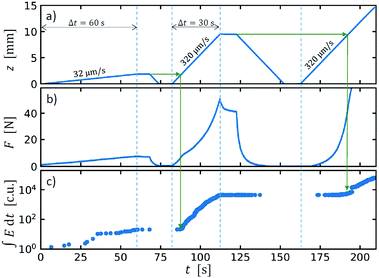
The compression protocol consists of three displacement controlled cycles illustrated in Fig. 3a. The first compression is a slow one with a displacement rate of ż = 32 μm s⁻¹ lasting 60 seconds corresponding to a strain rate of [small epsi, Greek, dot above] = 10% min⁻¹ (strain rate being calculated just as the displacement rate divided by the initial sample height). The first loading protocol up to 10% strain is based on a standard for thermal insulation materials.²⁹ The strain rate for the next loading phases is increased by the factor 10 in order to speed up the measurement. We observe the nearly linear increase in stress (which is proportional to the force F shown in Fig. 3b) and few individual acoustic emission events (Fig. 3c). After the loading has reached ε = 10% strain, the sample is unloaded with a faster rate ż = 320 μm s⁻¹ ([small epsi, Greek, dot above] = 100% min⁻¹). This return to the starting position is done manually with a few second delay after the loading has ended.

Fig. 3 The compression protocol consists of three cycles. (a) The displacement z data illustrates the linearity of the loading and the beginning and end of each loading cycle with dashed lines. (b) The measured force F corresponds to the loading cycles. (c) The cumulative acoustic emission energy is shown as dots when an event is detected. The data shows that there is a significant increase in acoustic event energy release rate when the compression exceeds the displacement of the previous cycle highlighted by green arrows.

The second compression cycle uses a faster displacement rate ż = 320 μm s⁻¹. Here, we observe clearly a non-linear stress–strain behavior and significantly more acoustic events. It also looks like the behavior changes as the strain exceeds the strain of the previous cycle and we start to compress the “virgin strain” portion of the sample. The green arrows highlight the location with a bump in the stress and significant increase in acoustic activity. The loading lasts for 30 seconds and the sample reaches ε = 50% strain. Again, after a few seconds we manually start the unloading ramp with the same faster displacement rate.

The third cycle is similar to the second one, except we compress until the stress limit of the load cell is reached. Also here we observe a bump in the stress data and a significant increase in acoustic activity as we move to “virgin strain” region of the sample.

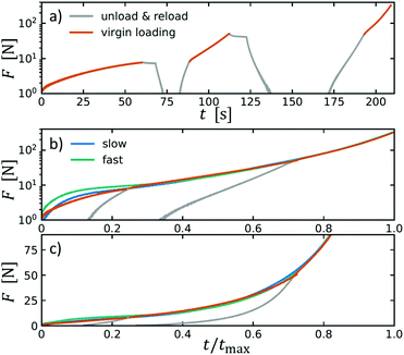
In the analysis that follows we have excluded all other parts except the virgin loading by stitching together the corresponding parts of the loading. This is done by attaching the end of one portion of virgin loading to the beginning of the next one as seen in Fig. 4. We can compare the resulting force curve to two reference experiments (which are not included in the further analysis) with continuous loading and different strain rates (slower one done with [small epsi, Greek, dot above] = 10% min⁻¹ and faster one with [small epsi, Greek, dot above] = 100% min⁻¹). This is done by normalizing the time-axis with the maximum time t_max (which for all experiments corresponds to the same stress). The force response is the same for both cases and we lose only a very tiny part of the acoustic emission data.

Fig. 4 The cyclic experiment can be re-scaled to a continuous loading. (a) There is a clear difference between when the strain exceeds the level of the previous cycle, highlighted in red. (b) Stitching the loading parts together overlaps with continuous compression experiments (blue and green). Here, the time is scaled. For the cyclic experiment the scaling is different for the first (slow) cycle. (c) The results appear the same in linear scale.

3 Results

3.1 Stress–strain response

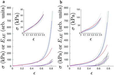
Fig. 5 shows the resulting averaged response for both sets of samples and zoomed-in views of the initial parts in the Insets. The curves are obtained from the cyclic experiments by joining together the parts of increasing compression. Ketoja et al.⁸ explained similar data for an extended set of trial points by making assumptions on the average order in which fiber segments (from a bond to subsequent bond) buckle during compression. The segment lengths a of the random network are exponentially distributed,where a₀ is the mean segment length. Long segments are generally less supported by the neighbouring ones and are expected to yield first. By assuming that on average fiber segments longer than a = a₀s(ε) undergo buckling and bending in order to scope with the mean strain ε, the following equation can be derived for the function s:⁸

[s(ε) + 1]exp[−s(ε)] = ε. (4)

On the other hand, the mean stress required for these bucklings to happen can be estimated using Euler's formula:⁸By solving s from eqn (4), we obtain the responsewhere W₋₁ is the second principal branch of the Lambert W-function, with one single fitting parameter σ₀. There are two main observations that one can draw based on Fig. 5. The first is that the theory fits the experiments up to a material-dependent strain/stress well. The agreement up to this point is very good for the BSKP samples that consist mainly of long fibers. Slightly larger deviation is seen for the CTMP samples probably due to their high fines content.³⁰ The second observation is that for both types of samples, the cumulative AE energy (depicted in Fig. 5 as a comparison) exhibits a strong increase in the region where the eventual discrepancy starts to be noticeable.

Fig. 5 (a) The stress–strain curves for the BSKP samples (light grey, decreases in strain from experiment cycles removed), their average (blue), the fitted model (red), the cumulative AE energies (dark grey) and their average (magenta). The fitting is done for the part below 50% strain. The Inset shows the same stress–strain response but zooming in on the part below 50% strain. (b) Same for the CTMP samples.

3.2 Acoustic emission and heterogeneous deformation

In cyclic compression tests, we observed a significant increase in the accumulated acoustic energy only when the compression exceeded the displacement of the previous cycle. Moreover, very few events were observed during the unloading of the sample between the cycles (see Fig. 3c). This suggests that acoustic events correspond to other failure mechanisms than fiber bending, which takes place also during unloading. The above mean-field theory based on fiber segment failures allows estimating the AE accumulation during compression. The proportion of buckled segments at strain ε is given byWe found the power α ≈ 3.0 of this function to describe the number of AE events with increasing strain (or stress), see Fig. 6. To compare the estimate for buckled segments to the AE event count we first normalize the event count n by the total number of events observed in an experiment n_tot. As the compression is stopped at a finite strain we do additional normalization with the predicted proportion of buckled segments at that maximum strain ε_max yieldingand similarly for the event rate . The normalized measured values of n* and ṅ* agree with the theoretical predictions e^−αs(ε) and , respectively, up to the strain level at which deviation between the measured and predicted stress–strain behavior was seen in Fig. 5.

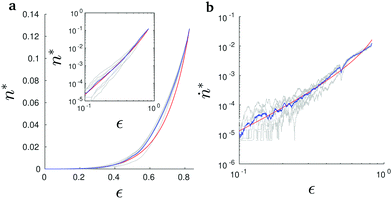Fig. 6 (a) Cumulative event counts (grey), their average (blue) and the theoretical prediction e^−αs(ε) (red) for varied strain ε. Here the measured values n have been normalized to according to eqn (8). The inset shows the same plot with logarithmic axes. (b) Event rates (grey) with the same normalization , their average (blue) and the theoretical prediction (red).

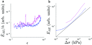
Moreover, the accumulated AE energy followed quite closely the total number of events for strains in the range of 10–50% (see Fig. 7a). In other words, the mean released acoustic energy per event was fairly constant in this region. For small strains below 10% this correspondence was lost but in this region there are only rather few events and the deformation is far from homogeneous as shown by Fig. 1b.

Fig. 7 (a) The ratio of the AE energy and event rates or in other words the average energy per AE event in a moving time window for BSKP (blue) and CTMP (magenta) samples. The average energy per event seems to be roughly constant until it starts increasing rapidly. This happens around the same point where the mean-field prediction for the stress–strain response starts to fail. (b) The deviation of the stress from the mean-field prediction versus the cumulative AE energy for the BSKP (blue) and CTMP (magenta) samples. The black line represents a power-law E_AE ∼ Δσ^1/2.

Beyond ε = 0.5, the energy integral increases rapidly (see Fig. 5). This coincides for both fiber structures with the deviations of the stress–strain curve from the mean-field like. Plotting the deviation

versus the AE energy integral shows that these two are roughly correlated in a power-law fashion with two different exponents close to 0.5 (see Fig. 7b). The consequence for the compression behavior of the foam formed structures is a hardening effect compared to the expected response (Fig. 5). The natural interpretation of this is the appearance of a different deformation mode, where further buckling events lead to localized avalanches and bursts of collective deformation. Similar avalanches have been earlier observed in simulations of non-bonded fiber networks.²⁶

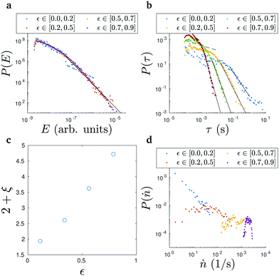
The statistics of the AE are quite different as regards the development with increasing strain. We therefore have divided the experiments into four strain bins (see Fig. 8) and consider the statistics of the events occurring in each strain bin separately. For the event energies we find in general P(E) ∼ E^−2.1, which is larger than what is found in the compression avalanches of other materials (Fig. 8a). Xu et al.³¹ have pointed out the possible existence of two different universality classes with more homogeneous materials tested (e.g. Vycor, wood¹⁹) resulting in a value of about 1.4 whereas more disorder leads in some cases (charcoal) to about 1.7, both in other words values again lower than 2.1. Here the fit is done as an maximum likelihood estimate to the set of all event energies (as the exponent does not change between the strain bins) and on the part of the distribution where the black line in Fig. 8a is drawn.

Fig. 8 (a) Distribution of the AE event energies from the BSKP samples divided into 4 strain bins. The black line is a power-law fit P(E) ∼ E^−2.1. (b) Distribution of the AE waiting times from the BSKP samples divided into the same 4 bins. The exponent of the power-laws fitted to the tail (solid black lines) seems to increase with strain. The dashed black line is power-law τ^−(1−ν) with ν = 0.6. (c) The exponents fitted to the tail of the waiting time distribution as a function of strain. There seems to be a linear increase in the exponent. (d) Distribution of the event rate in the same 4 bins.

The waiting time distribution evolves during the compression (Fig. 8b). As usual for AE waiting time statistics cut-off behavior is seen, so that at small strains the maximum times are larger and a power-law P(τ) ∼ τ^−(2+ξ) with an exponent close to −2 is found for the tail (Fig. 8c shows the results of fitting to distributions binned to strain windows). Again the fit is done as a maximum likelihood estimate and on the part where the solid black lines in Fig. 8b are drawn. The strong dependence of the distribution makes us expect that this is connected to the variations of event rate.¹⁴ If the probability distribution of the rates is broad enough this will show up in the waiting time distribution due to the rescaling of the waiting times even without any inter-event correlations as such. Fig. 6b demonstrates indeed that there is a change in the evolution of the rate, which grows approximately as a power-law in strain. Another typical feature of waiting time statistics in compression is that with small τ a small portion of the distribution seems to follow P(τ) ∼ τ^−(1−ν), here ν being close to 0.6 as seen from the dashed black line in Fig. 8b. This is related to Omori-type aftershock sequences with an event rate proportional to t^−(1−ν) when time is measured from the mainshock,¹⁴ and indicates correlations in the waiting times at short times. The tail of the P(τ) is on the other hand linked to the rate distributions, Fig. 8d, which has the easy interpretation that the probability of a large waiting time is dominated by the periods in the time series when the event rate is small.

4 Conclusions

We have studied the compression of foam formed fiber-based low-weight structures. These materials deform in their own, particular way which can be to a quite large degree be described by mean-field arguments. This includes not only the stress–strain behavior but also the measured accumulated AE events during compression. We found an explicit mathematical coupling between these two properties.

However, as one might expect, with increasing compression the deformation behavior changes. The main empirical observation is the hardening of the response as seen in the stress–strain curve, compared to the mean-field-picture. This change in behavior can be easily detected by AE observations. In a strain region around 50% the avalanche activity increases tremendously.

The AE bursts exhibit energy statistics that are not much dependent on the strain window of observation, thus on the main mode of deformation. Instead, the temporal, waiting time statistics show substantial changes. This is connected with the ramp-up of the AE event rate, and our results show that this is the fundamental reason behind the change in the waiting time statistics. We thus conclude that these materials differ from what has thus been observed in “non-soft” matter, including wood.

As the mean-field argument is very general, it will be interesting to seek for other similar systems where it could be applicable. In this context, a further topic is to investigate mechanisms by which the theory breaks because of possible collective or other complex phenomena, as seems to happen here at larger strains.

Conflicts of interest

There are no conflicts to declare.

Acknowledgements

We thank Eduard Vives for useful discussions. We acknowledge the financial support from the Academy of Finland through the Centers of Excellence program (Project No. 251748), and the postdoctoral grant 308235 (J. K). M. A. acknowledges support from the European Union Horizon 2020 research and innovation programme under grant agreement No. 857470 and from European Regional Development Fund via Foundation for Polish Science International Research Agenda PLUS programme grant No. MAB PLUS/2018/8. The work has been partly supported by the European Regional Development Fund (grant number A73089, A73092). We are also grateful for the support by the FinnCERES Materials Bioeconomy Ecosystem. We acknowledge the computational resources provided by the Aalto University School of Science “Science-IT” project.

Notes and references

1. B. Radvan and A. P. J. Gatward, Tappi J., 1972, 55, 748–751.
2. J. Lehmonen, P. Jetsu, K. Kinnunen and T. Hjelt, Nord. Pulp Pap. Res. J., 2013, 28, 392–398.
3. A. Madani, S. Zeinoddini, S. Varahmi, H. Turnbull, A. B. Phillion, J. A. Olson and D. M. Martinez, Cellulose, 2014, 21, 2023–2031.
4. M. Alimadadi and T. Uesaka, Cellulose, 2016, 23, 661–671.
5. S. Burke, M. Möbius, T. Hjelt and S. Hutzler, Cellulose, 2019, 26, 2529–2539.
6. A. M. Al-Qararah, A. Ekman, T. Hjelt, J. A. Ketoja, H. Kiiskinen, A. Koponen and J. Timonen, Colloids Surf., A, 2015, 482, 544–553.
7. T. Komori and K. Makishima, Text. Res. J., 1977, 47, 13–17.
8. J. A. Ketoja, S. Paunonen, P. Jetsu and E. Pääkkönen, Materials, 2019, 12, 384.
9. T. Sormunen, A. Ketola, A. Miettinen, J. Parkkonen and E. Retulainen, Sci. Rep., 2019, 9, 4258.
10. G. Subramanian and C. R. Picu, Phys. Rev. E, 2011, 83, 056120.
11. M. Alimadadi, S. B. Lindström and A. Kulachenko, Soft Matter, 2018, 14, 8945–8955.
12. M. J. Alava, P. K. V. V. Nukala and S. Zapperi, Adv. Phys., 2006, 55, 349.
13. L. Girard, J. Weiss and D. Amitrano, Phys. Rev. Lett., 2012, 108, 225502.
14. J. Baró, A. Corral, X. Illa, A. Planes, E. K. H. Salje, W. Schranz, D. Soto-Parra and E. Vives, Phys. Rev. Lett., 2013, 110, 088702.
15. F. Kun, I. Varga, S. Lennartz-Sassinek and I. G. Main, Phys. Rev. Lett., 2014, 112, 065501.
16. S. Lennartz-Sassinek, I. G. Main, M. Zaiser and C. C. Graham, Phys. Rev. E, 2014, 90, 052401.
17. G. Nataf, P. Castillo-Villa, J. Baró, X. Illa, E. Vives, A. Planes and E. K. H. Salje, Phys. Rev. E, 2014, 90, 022405.
18. J. Weiss, L. Girard, F. Gimbert, D. Amitrano and D. Vandembroucq, Proc. Natl. Acad. Sci. U. S. A., 2014, 111, 6231–6236.
19. T. Mäkinen, A. Miksic, M. Ovaska and M. J. Alava, Phys. Rev. Lett., 2015, 115, 055501.
20. J. Vasseur, F. B. Wadsworth, Y. Lavallée, A. F. Bell, I. G. Main and D. B. Dingwell, Sci. Rep., 2015, 5, 13259.
21. J. Baró, P. Shyu, S. Pang, I. M. Jasiuk, E. Vives, E. K. H. Salje and A. Planes, Phys. Rev. E, 2016, 93, 053001.
22. L. Viitanen, M. Ovaska, M. J. Alava and P. Karppinen, J. Stat. Mech.: Theory Exp., 2017, 053401.
23. J. Baró, K. A. Dahmen, J. Davidsen, A. Planes, P. O. Castillo, G. F. Nataf, E. K. Salje and E. Vives, Phys. Rev. Lett., 2018, 120, 245501.
24. F. Renard, J. Weiss, J. Mathiesen, Y. Ben-Zion, N. Kandula and B. Cordonnier, J. Geophys. Res., 2018, 123, JB014964.
25. C. Vu, D. Amitrano, O. Plé and J. Weiss, Phys. Rev. Lett., 2019, 122, 015502.
26. R. C. Picu and G. Subramanian, Phys. Rev. E, 2011, 84, 031904.
27. J. Blaber, B. Adair and A. Antoniou, Exp. Mech., 2015, 55, 1105–1122.
28. A. Patist, S. S. Bhagwat, K. W. Penfield, P. Aikens and D. O. Shah, J. Surfactants Deterg., 2000, 3, 53–58.
29. Standard EN826:2013, Thermal insulating products for building applications – Determination of compression behaviour, 2013.
30. T. Pöhler, J. A. Ketoja, T. Lappalainen, V.-M. Luukkainen, I. Nurminen, P. Lahtinen and K. Torvinen, Cellulose, 2020 DOI:10.1007/s10570-020-03263-x.
31. Y. Xu, A. G. Borrego, A. Planes, X. Ding and E. Vives, Phys. Rev. E, 2019, 99, 033001.

---