Autonomous analysis to identify bijels from two-dimensional images

Abstract

Bicontinuous interfacially jammed emulsion gels (bijels) are novel composite materials that can be challenging to manufacture. As a step towards automating production, we have developed a machine learning tool to classify fabrication attempts. We use training and testing data in the form of confocal images from both successful and unsuccessful attempts at bijel fabrication. We then apply machine learning techniques to this data in order to classify whether an image is a bijel or a non-bijel. Our principal approach is to process the images to find their autocorrelation function and structure factor, and from these functions we identify variables that can be used for training a supervised machine learning model to identify a bijel image. We are able to categorise images with reasonable accuracies of 85.4% and 87.5% for two different approaches. We find that using both the liquid and particle channels helps to achieve optimal performance and that successful classification relies on the bijel samples sharing a characteristic length scale. Our second approach is to classify the shapes of the liquid domains directly; the shape descriptors are then used to classify fabrication attempts via a decision tree. We have used an adaptive design approach to find an image pre-processing step that yields the optimal classification results. Again, we find that the characteristic length scale of the images is crucial in performing the classification.

---

1 Introduction

Physics has a close relationship to machine learning, especially with respect to the development of neural networks.^1–3 Today, there are a number of areas of physics in which machine learning is used extensively.¹ In soft matter physics, this is especially true for the design of soft materials.⁴ Examples include the inverse design of self-assembled materials⁵ and the investigation of protein folding landscapes.⁶ In addition to this, machine learning has been used to design experiments themselves⁷ and to identify crystal structures from molecular simulations or particle tracking data.^8,9

In this study, we are using machine learning to classify the outcome of experiments. A bijel is a “bicontinuous interfacially jammed emulsion gel”: a special class of particle-stabilised emulsion prepared by arresting demixing that occurs via spinodal decomposition.^10,11 The end result is a bicontinuous structure with the two phase-separated liquids intertwined and stabilised by the adsorption of colloidal particles to the liquid–liquid interface. This adsorption is effectively irreversible due to the high attachment energy of the particles to the interface,¹² so the structure is jammed once the particles are closely packed and is stable against further coarsening.

The tortuous, interconnected spinodal pattern is what characterises bijels and also what makes them interesting materials for a number of potential applications, including fuel cells,¹³ controlled release devices¹⁴ and tissue engineering.¹⁵ A bijel has a single characteristic length scale, which is the width of the liquid channels. This can also be seen in the structure factor of a system undergoing spinodal decomposition, which shows a single intensity peak at any given time during demixing.

We are interested in simple methods to quickly separate successful bijel samples from failed ones in order to expedite production. A simple tool for bijel classification could be widely used to verify if a bijel fabrication has been successful. Because of the difficulty in manufacturing them, research is ongoing into easier methods for making bijel structures, such as solvent transfer induced phase separation¹⁶ and direct mixing.^17,18 This area of research provides even more potential applications for a bijel classification tool, and in fact some initial attempts have been made to evaluate potential bijel structures using an empirical cost function.¹⁹

We make use of data from a previous study of the mechanical properties of bijels under compression,²⁰ in which there was a great need to verify the quality of bijel samples before they were subjected to centrifugal compression. This verification involved assessing each sample under a confocal microscope and we therefore have a large number of confocal images of both successful and failed bijel samples on which we can train and test our classification methods.

Current bijel research tends to focus solely on successful samples, so there is little public record of methods used for determining whether a bijel synthesis has been successful or not. We assume that most samples are assessed by the experimenter by eye both macroscopically and (predominantly) microscopically during imaging. Additionally, there are a number of methods used to quantify different aspects of a bijel, some of which can be used to identify failed bijels as well as to characterise successful ones. The local Gaussian (K) and mean (H) curvatures of a bijel structure have been found to have strong peaks at K < 0 and H = 0, respectively.^21,22 An alternative three-dimensional image analysis method of ‘region growing’ is used to determine whether the structure is bicontinuous:²² an important requirement of a bijel.

These methods could all be used to help identify successful bijel samples. However, as these methods all require a suitable three-dimensional image of the bijel (such as a confocal stack or a CT scan of a polymerised bijel), as well as significant computational workload, there is much scope for a more versatile, high throughput alternative. Here we assess the sample classification performance of machine learning methods applied to confocal micrographs of only two dimensions.

2 Methods

2.1 Image processing

Our confocal images are from a selection of successful and unsuccessful bijel samples. Each image is composed of a liquid (fluorescein-doped ethanediol) and a particle (silica modified with hexamethyldisilazane, doped with rhodamine B) channel. These two different fluorescent dyes were used so that the particles and the liquid could be imaged separately.²⁰ The images from the two channels were processed independently to obtain the structure factor and autocorrelation function of each image and channel.

Two functions were derived from the Fourier transform of the image. Firstly, the structure factor was calculated by radially averaging the Fourier transform. Secondly, the autocorrelation function was also calculated from the Fourier transform by multiplying it with itself under the transformation r → −r, then performing an inverse Fourier transform on the result. We have effectively convolved the image with its reflection, which gives us the correlation function of the image with itself, i.e. the autocorrelation function:

We performed this image processing in Python using the skimage package²³ to read in the two separate channels for each image and using the fast Fourier transform methods available in the standard scipy package.

2.2 Machine learning

We used R to perform all of our machine learning, primarily via the caret package,²⁴ which contains a wide array of machine learning tools and algorithms. In order to achieve optimal classification performance, we tested a number of different machine learning classification algorithms with a variety of potential predictors obtained from the structure factor and autocorrelation functions of our images. Three algorithms were particularly suited to our data and approaches: these are described below and detailed further in the ESI.† As well as testing different algorithms, we were always attempting to reduce the number of predictive variables used, because an optimal model should also be a minimal one. In this project, we never work with a large number of variables and the optimal model could therefore be easily found without the need for variable reduction methods, such as principal component analysis or ridge regression.

2.2.1 k-Nearest neighbours algorithm. The k-nearest neighbours (KNN) algorithm is one of the simplest and therefore most commonly used machine learning classification algorithms. This method classifies an unknown point in variable space based on a “vote” of its nearest k neighbours of known classification. The number of neighbours is tuned to improve the fit of the model.²⁵

In order to avoid inadvertently weighting some variables more than others, this algorithm requires that all variables are normalised so that they are of comparable scale. As long as this is done, the absolute scale of the variables is unimportant. Each variable is usually therefore normalised by the mean of its value over the whole training set.

2.2.2 Logistic regression. The logistic regression algorithm is in some ways more versatile than k-nearest neighbours because it can give a probability of the sample belonging to a class, which allows a classification to be tuned to achieve a suitable balance of false positives and false negatives depending on the needs of any application. We find the probability p(X) of a sample being a bijel given a set of predictive variables X = (X₁, X₂,…X_i) by fitting a linear logit function:using the maximum likelihood method to find values of β that fit the training data provided.²⁵ The form of this function means that the probabilities p(X) are bounded between 0 and 1, as required.

2.2.3 Decision trees. The decision tree algorithm can be used for both classification and regression, but here we focus on classification trees. In order form a classification tree, we take an approach known as recursive binary splitting, wherein we start at the ‘top’ of the tree and split the predictor space in two, such that the classes are best separated. We then repeat the splitting process down both possible branches, and we stop growing our tree when further branching leads to no significant improvement in the classification error.²⁵ The final tree shows us the proportion of a particular category in each end node as well as the splits that have been chosen, for example in Fig. 9(a).

2.2.4 Errors and cross-validation. We define our classification error rate as the percentage of test images that were misclassified. When fitting any model, the first comparison to make is to the null error rate, which is the error rate obtained by classifying every sample as the most popular class. In our case, the most common class is the successful bijels, and our null error rate is 31.9% misclassification.

In general, the application of machine learning to a problem requires splitting data into two sets: one for training and one for testing. The algorithm is first trained on the training data, then the final model output from this is used to predict the outcome of the test data and the error on these predictions is used to compare models. This approach is required in order to ensure that the model is not over-fitted to the fluctuations and quirks of a specific dataset, and can be effectively used to predict future data from outside the training set.

As we have a relatively small dataset (135 samples) we used cross-validation to make the most of this data without having to set aside a large chunk for testing our models separately. Cross-validation requires splitting the data into n equally sized sections, or folds. One of these folds is set aside for testing, and the model is trained on the remaining n − 1 folds. The trained model is then tested on the fold set aside, and this result is stored. The process is repeated n times, until each fold has been used once as a test set. The results of all n tests are combined to give a cross-validated error rate, which is a combination of all iterations and gives a final error effectively based on the whole dataset as a test set, but avoiding the problem of over-fitting. This method is often used to tune model parameters within a single machine learning method, and is included in the algorithm. The error quoted in the model output is then the cross-validated error. Except where stated otherwise, we used 10-fold cross-validation in all of our model fitting.

2.3 Efficient global optimisation

Our secondary approach was to categorise the micrographs while avoiding the averaging associated with autocorrelation functions and structure factors. Instead, the distribution of shapes within the images was separately analysed. The shapes of interest in our images are the liquid domains; these can be simplified and isolated using a grey-scale threshold. The resulting images show one liquid domain as black and the other as white. We then use the shape filter plugin for ImageJ to obtain descriptors of our liquid domain shapes such as: the area per perimeter, the fractal dimensionality, the solidity, and many others.^26,27 This approach would be advantageous if it captured details valuable for classification which autocorrelation functions and structure factors lose.

In order to achieve the optimal performance of the classification via the domain shape, we have carried out a thorough exploration of how the error rate is influenced by an image pre-processing step. Here we have used a decision tree combined with six-fold cross-validation as the final classification step. The great strength of this approach is that the succession of division criteria can subsequently be read and interpreted. The decision tree will effectively tell us what the optimisation step, described below, actually achieved. Such information would be more difficult to access using an alternative classification algorithm.

The control parameters for our pre-processing are: the size of a median filter, the upper and lower limits of a band pass filter of the grey-scale images, and an upper bound on the size of small liquid domains to ignore once the images have been thresholded. The effect of these pre-processing steps on seven example images is shown in the ESI.†

We have used an approach variously known as efficient global optimisation, adaptive design and kriging to explore this parameter space.^28,29 We want our exploration to yield the lowest possible error rate for our classification of bijel images. Efficient global optimisation begins with some well-spaced trial pre-processing approaches; these are used to train a machine learning algorithm. This algorithm could direct us to a prediction of the pre-processing parameters for which the classification error rate is apparently immediately minimised. This will, almost certainly, be a local minimum. In efficient global optimisation a composite parameter directs the search favouring a low error rate and also driving the exploration towards uninvestigated regions of parameter space, as described in the ESI.†

3 Results

3.1 Data

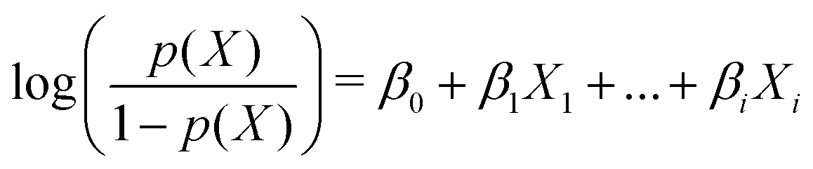
Fig. 1(a) shows the outcome (successful bijel or not) of a representative set of 135 bijel experiments, and their dependence on key compositional parameters. The HMDS (hexamethyldisilazane) content controls the particle wettability, and the nitromethane mass fraction (relative to the ethanediol content) acts as a proxy for the distance of the system from the critical composition, which is at a mass fraction of 0.640.²⁰ Many of the successful samples are clustered around this composition. Nonetheless, it is important to notice that the outcome of the experiment (bijel or non-bijel) is not guaranteed to be the same for the same experimental parameters. In other words, identical composition parameters do not always give identical outcomes. This is why an image analysis classification approach is valuable.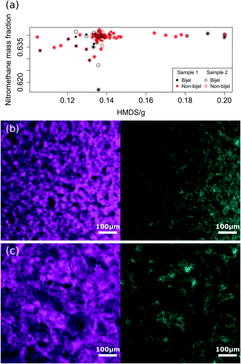

Fig. 1 Experimental data used in this project. Panel (a) shows the outcome of 135 attempted bijel samples indicating whether a successful bijel was created as a function of particle wettability and nitromethane mass fraction. Where samples 1 and 2 have the same composition, they are made from the same sample batch split in half. Panels (b) and (c) show examples of a successful and an unsuccessful bijel respectively. The ethanediol phase (liquid channel) is shown in magenta on the left, and the stabilising silica particles (particle channel) are in cyan on the right.

We can see this problem in Fig. 1(b) and (c), which show images from two compositionally identical samples. These were created by splitting one sample in half and applying the same experimental protocol to each half. From consideration of the whole sample from which these images were taken, the one in Fig. 1(b) was classified as a bijel, and Fig. 1(c) is not a bijel, as is evident from the abundance of droplets in the image.

Fig. 2 shows examples of the particle channel structure factor (a) and liquid channel autocorrelation function (b) of a bijel and a non-bijel. As the structure factor is much noisier than the autocorrelation function (in both channels but particularly the particle one), it was less useful for providing a wide range of variables to test in our models.

Fig. 2 Comparisons of representative example bijels (in red) and non-bijels (in black) in terms of their structure factors and autocorrelation functions. Panels (a) and (b) show the structure factors and autocorrelation functions of the liquid channel images respectively. Panels (c) and (d) show the structure factors and autocorrelation functions of the particle channel images.

Fig. 3 shows how the variables in our final machine learning models can individually distinguish an image of a bijel from an image of a failed bijel. Plots like these were made for a number of potential variables which were chosen to represent key features in the functions, and were used to rule out variables that clearly showed no distinction between bijels and non-bijels.

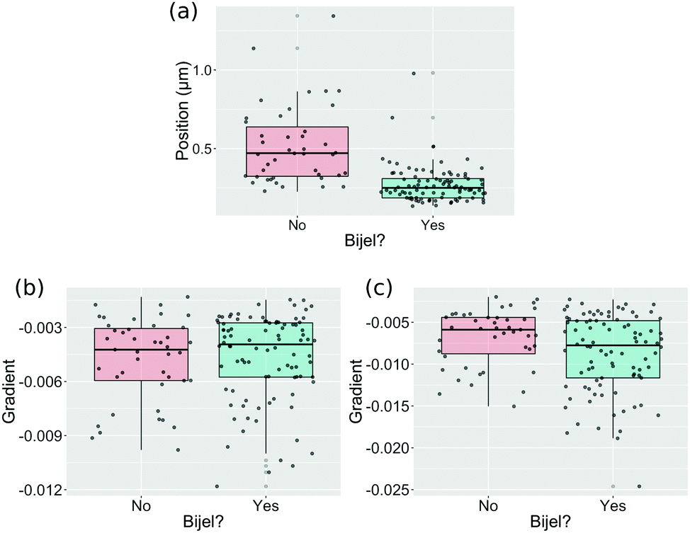Fig. 3 Box-and-jitter plots of the three variables included in the final combined-channel model. These plots show how the values of the variable are distributed for bijels and non-bijels. Jitter is added in the x-axis so all points can be seen. Panel (a) shows the position of the first turning point in the liquid channel autocorrelation function. Panels (b) and (c) show the gradient of the first 10 and 20 points, respectively, in the particle channel autocorrelation function.

It is clear that the position of the first turning point in the autocorrelation function of the liquid channel is a strong predictor on its own. Other variables, such as the gradient of a straight line fit to the first 10 (Fig. 3(b)) and first 20 (Fig. 3(c)) points of the particle channel autocorrelation function, show only a small difference between bijel and non-bijel samples and prove to be significant only when combined with other predictors. These two variables both approximate the initial slope of the autocorrelation function but both were assessed individually because the distributions shown in the box-and-jitter plots are sufficiently different, and because if they do give the same information then one will be eliminated when we remove ineffective variables.

The usefulness of these variables that seem less important is not unexpected, as we are analysing a multidimensional variable landscape and there is no need for a useful predictor to classify a bijel image alone. Instead, our approach requires only that any variables included in the final model are useful for reducing the overall classification error rate. This keeps the number of variables as low as possible while still maximising performance.

3.2 Machine learning results

3.2.1 Liquid channel model. We first trained the model using 7 predictive variables describing the shapes of the autocorrelation function and structure factors of the liquid channel images. We tested a number of algorithms and found that the k-nearest neighbours algorithm consistently gave the best results for these images, so we continued to use this model for further refinement.

Once we had this base model, we worked to improve its classification performance. We revisited the variables we had chosen, and assessed their success in differentiating between bijel and non-bijel samples. As we were working with only a few predictive variables, we opted to assess the impact of each variable individually rather than relying on methods such as principal component analysis. This gave us the benefit of knowing exactly how each variable affected the final performance of the model.

We calculated the significance of each variable in our model using the f-statistic:²⁵ a measure commonly used to compare models related to the ratio between the variance in the data that is explained by this variable and the variance that is not. We used these values to rank our predictive variables in order of significance, and iteratively refit the model removing the least significant variable each time. This allowed us to reached a minimal model with maximal performance.

Of the 7 variables used to fit the initial models, we discovered that the position of the first turning point in the autocorrelation function was the most significant predictor, followed by the initial gradient of the structure factor. Upon reducing the number of variables in the model, we found a decrease in error with each reduction, starting at 21.5% and achieving 16.6% when the model was reduced to only the most significant variable. Although we have identified a single useful indicator, and could therefore consider classifying bijels based on a threshold value of this variable, the application of machine learning is still required for two reasons. Firstly, the machine learning algorithms generally allow for more complex decision boundaries than a single split at a certain value. This can be seen in Fig. 4(b), with non-bijels predicted at position (*) as well as values above position (†). Secondly, the benefit of developing a machine learning method is that once a good model is chosen it can be re-trained on a different set of data in order to make predictions about a different bijel system. If we aimed to identify bijels by simply setting a threshold for the value of this autocorrelation turning point, this could not be generalised to other bijel systems.

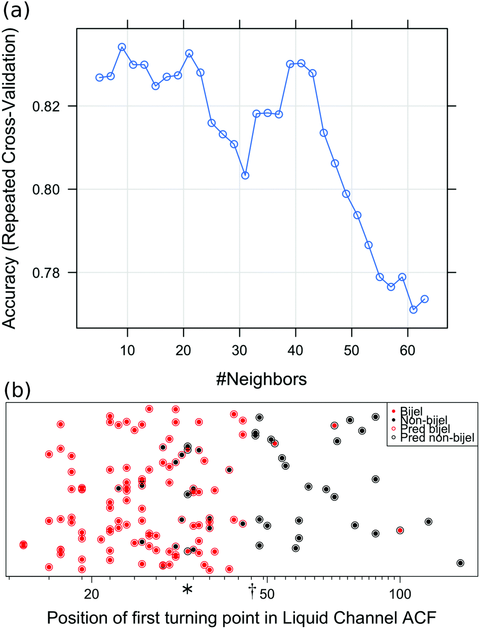Fig. 4 Results from the best liquid channel KNN model. Panel (a) shows cross-validation results for the final KNN fit to the liquid channel images, and how the cross-validated accuracy of the model changes with the number of neighbours used in the classification. Panel (b) shows the predicted (open circle) and true (filled circle) bijel classifications for each sample in the dataset, with y-axis jitter added as only one variable was used in the model. Predictions were output from the final liquid channel KNN fit.

Fig. 4 shows the outcome of the final k-nearest-neighbours model fitted to the liquid channel images. Fig. 4(a) shows how the error rate varies depending on the number of nearest neighbours used in the model. We see that k = 9 gives the best performance because it gives the highest accuracy, so this is chosen for the final model. Fig. 4(b) shows the predictions made by this model compared to the true classifications. The error rate for this prediction model is 16.6%.

3.2.2 Particle channel model. Once the results using the liquid channel alone were no longer improving, we turned to the particle channel for more information that could help to identify a bijel sample. We first investigated this channel on its own in order to understand which variables would be useful predictors.

Using 5 initial predictive variables, in this case all derived from the autocorrelation function due to the noisiness of the structure factor, we tested various machine learning algorithms and found that logistic regression out-performed its competitors. The logistic regression generates a probability of a sample being a bijel and being a non-bijel, and the sample is classified as a bijel if Pr(bijel) ≥ Pr(not bijel). We also considered the support vector machine algorithm²⁵ as a strong contender in this test since it gave no significant improvement over logistic regression. However, logistic regression has the benefit that the fits can be used directly to determine the significance of each variable. Therefore, we will not pursue the support vector machine algorithm further here.

For this channel, our initial predictors were all associated with the autocorrelation function because the structure factors for the images in this channel were much noisier and less consistent than those of the liquid channel. From the logistic regression fit, we found that the most significant of these predictors were the gradients of the first 10 and first 20 points of the autocorrelation function, followed by the value of the autocorrelation function at its first turning point. The least significant predictors were the number of turning points and the position of the first turning point in the autocorrelation function. Removing these two variables from the model led to an error change from 20.4% to 20.6%: a small drop in performance. However, removing the turning point value, leaving only the two gradient variables, led to a much improved error of 17.6%. Further reduction of the model led to a large increase in the error.

Fig. 5 shows the outcome of the best performing model fitted to particle channel images. This model was a linear logistic regression of two variables: the straight line gradients of the first 10 and first 20 points of the autocorrelation function. The error rate for this model is 17.6%, which is worse than that of the liquid channel model. In order to seek further improvements, we combined the two channels together for a final model.

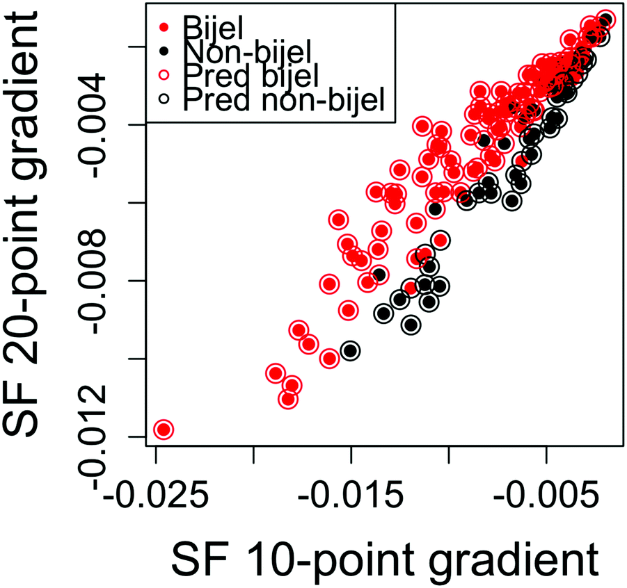Fig. 5 Results from the best particle channel logistic regression model. Predicted (open circle) and true (filled circle) bijel classification results for each sample in the dataset. Predictions were output from the final particle channel model and plotted as a function of the two variables in the model.

3.2.3 Combined model. We combined the optimal variables from both the liquid and particle channels, and again tested a number of algorithms in order to identify which performed best. We unsurprisingly found that the KNN and logistic regression methods gave the best performance. Of these, logistic regression gave the lower error so we explored this model a little further by assessing the impact of non-linear dependencies of the logit function on the predictive variables. This consistently decreased the performance confirming that the linear logistic regression was the most suitable version.

In order to confirm that the inclusion of all three previously chosen variables gave for the best result, we tested all previously untried combinations of pairs of these variables using both the KNN and logistic regression algorithms. We found that, with both the KNN and logistic regression algorithms, the inclusion of all three variables gave the best performance. Interestingly, reducing the number of variables made little to no difference to the performance of the KNN method, but with logistic regression the inclusion of all three variables was vital for achieving the optimal performance and allowing it to outperform the KNN algorithm and the single-channel models.

Fig. 6 shows the outcome of the best performing model fitted using variables from both the liquid and particle image channels. We achieved a 14.6% error: our best performance with this approach and a significant improvement from the results of either channel individually. Once the variables have been selected, this model can be trained and used to classify new images in a matter of seconds. This approach therefore provides an effective method of quickly categorising bijel images.

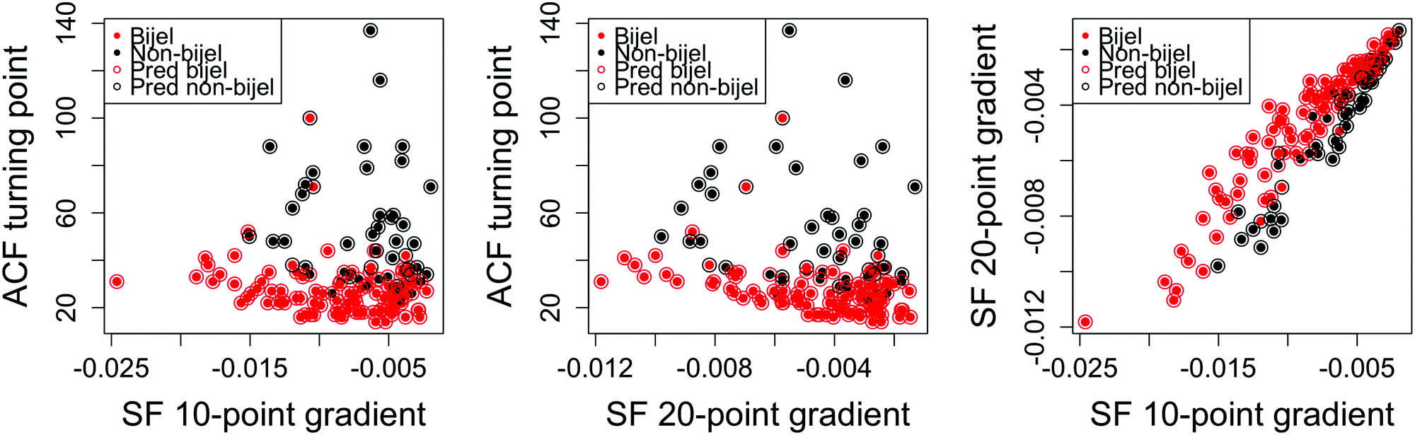Fig. 6 Results from the final logistic regression model using both liquid and particle channels. Predicted (open circle) and true (filled circle) bijel classification results for each sample in the dataset plotted for each possible pair of the three variables used in the model.

3.2.4 Model validation. Once our final model was chosen, we used a number of tests to assess the performance of the model further. This allows us to gain more information on the quality of the final model besides the classification error, and to verify that it is a useful classification tool.

Fig. 7 is a ROC (receiver operator characteristic) curve showing the balance between the true and false negative results as we change the probability threshold above which a sample is classified as a bijel. The straight line signifies the expected result from a random guess. The point (0,1) is the error-free point, where all of our classifications would be correct. The area underneath the curve is used to measure the quality of the model as a test, where an area of 1 represents a perfect test and a test with an area of 0.5 is worthless. Our test has an area of 0.912, which is generally viewed as excellent.

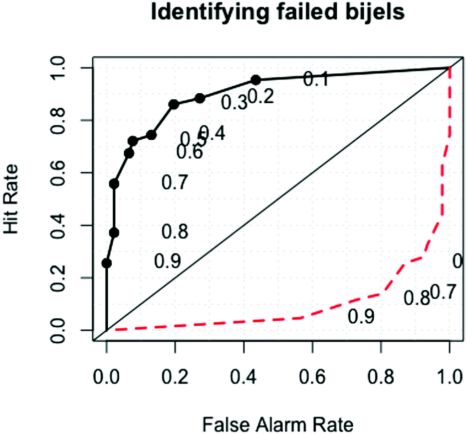Fig. 7 Receiver operator characteristic curve for the final model fit used to measure the quality of the fitted model. This shows how the true and false negative results change as a function of the probability threshold at which a sample is classed as a non-bijel. The area beneath the curve is 0.912, indicating an excellent model.

As a test of whether the images carry useful information about the classification of the samples, we randomised the classification of the images. Fig. 8 shows the error rate for 1000 iterations of the final model. This model was used to classify the same images that were used for training but with random (and thus incorrect) labels of bijel and non-bijel. The total number of each label was not changed. Comparison to the error rate of our best model (in purple) shows that the predictive power of the model is indeed significant and relies on the images being correctly classified. Therefore, we can be sure that we are indeed identifying features of images from bijel samples rather than random similarities between images.

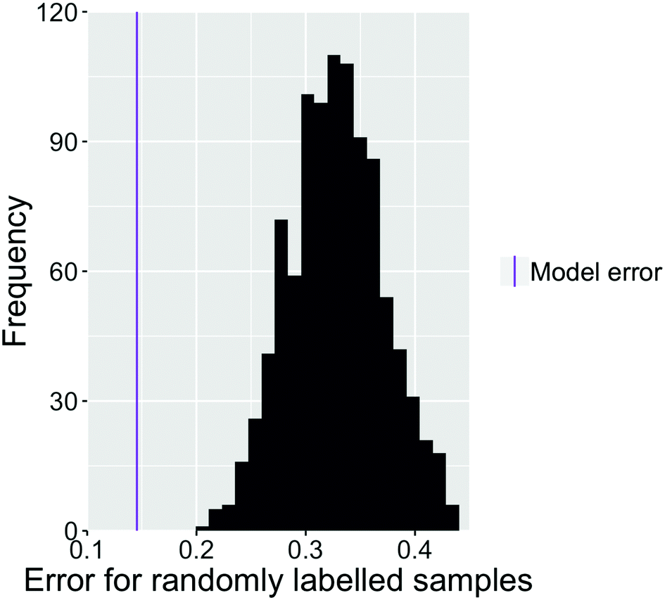Fig. 8 Histogram of the error rate for 1000 iterations of the final model fitted with random bijel labelling. These errors are all significantly higher than the error achieved with our model fit to the true data, shown as a purple line.

We assessed the performance of the fitted model on multiple images from the same sample. These additional images were taken from two of the 135 experimental samples used in the training of the model, one a bijel and one not. The model was used to predict whether these new images were from a bijel sample or not, and these predictions were correct for 6 of 8 bijel images, and all of the 11 non-bijel images tested.

As a final test of our machine learning approach, we applied it to a new set of data. This data was from samples of the same general composition but using a different batch of particles which led to different results in the final sample. Our machine learning models show that the two sets of samples have different properties: testing the previously trained model on the new data gave an error rate of 39%. In contrast, when we use the same approach and train a k-nearest neighbours algorithm with the same 3 predictive variables on the new data, we obtain a model that can identify a bijel with only a 13% error rate. This shows that the machine learning approach developed here can be used on a variety of different bijel systems and confirms that the models require re-training for each new system, since the characteristic length scale changes.

3.2.5 Efficient global optimisation approach. Finally, we look at using an efficient global optimisation approach. This involves simply analysing the distribution of shapes within the images. The classification error rate was investigated for various image pre-processing steps. Prior to optimised pre-processing, our typical error rate using this method was 27% of the images misclassified. Following the investigation of dozens of combinations of pre-processing parameters we reduced the error rate to 12.0%. The classification was based on the shape descriptors: fractal dimensionality, area per perimeter, Feret mean diameter, and the solidity. It is important to note that most of these descriptors are, to some extent, characterising the length-scale of the domains. The optimal image pre-processing approach (corresponding to a 12% failure rate) had no median filtering and modest amounts of low and high pass filtering. The shape size cut-off removed objects of size less than 415 pixels, which is surprisingly large.

As shown in Fig. 9(a), the decision tree initially uses several parameters to classify the images. Even then the performance is poor. An example of the problem is shown in Fig. 10(a), which shows a box plot of the shape descriptor area per perimeter. There is very strong overlap between this characteristic for bijel and non-bijel samples. Once the pre-processing has been optimised this box plot changes markedly (see Fig. 10(b)). Now the overlap between bijel and non-bijel samples is considerably reduced. The decision tree now harnesses this good separation (see Fig. 9(b)). The tree divides bijel from non-bijel samples relatively cleanly relying on the area per perimeter parameter alone. This makes classification more straightforward and therefore more likely to be accurate, as evidenced by the drop in error rate from 27% to the final value of 12.0%.

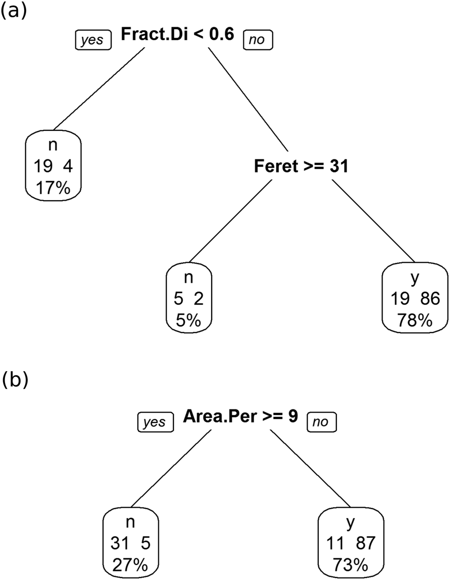Fig. 9 Example outcomes from applying the decision tree algorithm to variables before (a) and after (b) optimised pre-processing. The samples have been categorised based on the values of fractal dimensionality (Fract.Di), Feret mean diameter (Feret) and area per perimeter (Area.Per). A ‘y’ result indicates that a sample in the node is predicted to be a bijel and an ‘n’ that it is a non-bijel. The two numbers in each node show the number of non-bijel and bijel training observations that fall in the node respectively. The percentage in each node shows the percentage of all training observations present in the node.

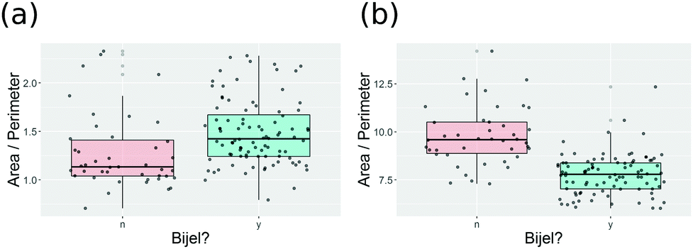Fig. 10 Box-and-jitter plots of an example variable: area per perimeter. Panel (a) shows this variable with only minimal pre-processing, and (b) shows it after pre-processing optimised via efficient global optimisation.

4 Conclusions

We have found that machine learning can be a powerful tool for use in the identification of bijels from a two-dimensional confocal image. We have used two different but similar approaches, and found both of them to be interesting. The first approach, which involved processing the images to get the autocorrelation function, was optimised to a classification accuracy of 85.4% and allows for rapid classification. As our images contained separate information about two of the three phases present in the bijel, we found that we were able to gain even more classification performance using both channels compared to using one channel alone.

The second approach, which involved optimising the pre-processing of the image, gave a better classification accuracy of 88.0%. Using this approach, it was particularly clear that the length scales present in the sample are important in the classification of the bijel. The downside to this approach compared to using the autocorrelation function is that the optimisation of the pre-processing is more time-consuming and requires more human input than simply calculating the autocorrelation function.

As the machine learning algorithms require very little computation time and minimal human intervention once the optimal model has been found, these approaches provide an opportunity to easily identify a bijel from a two-dimensional image. Even without information from a third dimension, bijels can be identified with reasonable accuracy showing the usefulness of machine learning for applications such as this.

Conflicts of interest

There are no conflicts to declare.

Acknowledgements

E. M. G. thanks EPSRC for PhD funding with the Condensed Matter Centre for Doctoral Training (CM-CDT) under grant number EP/L015110/1. K. A. M. thanks EPSRC for PhD studentship funding with the Condensed Matter Centre for Doctoral Training (CM-CDT) under grant number EP/G03673X/1. We also thank Iain Muntz for his assistance with calculating autocorrelation functions.

References

1. G. Carleo, I. Cirac, K. Cranmer, L. Daudet, M. Schuld, N. Tishby, L. Vogt-Maranto and L. Zdeborová, Machine learning and the physical sciences, 2019, http://arxiv.org/abs/1903.10563.
2. E. J. Gardner, D. J. Wallace, N. Stroud, E. J. Gardner, B. Derrida, H. Gutfreund and I. Yekutieli, J. Phys. A: Math. Gen., 1988, 21, 257–270.
3. J. J. Hopfield, Proc. Natl. Acad. Sci. U. S. A., 1982, 79, 2554–2558.
4. A. L. Ferguson, J. Phys.: Condens. Matter, 2018, 30, 043002.
5. M. R. Khadilkar, S. Paradiso, K. T. Delaney and G. H. Fredrickson, Macromolecules, 2017, 50, 6702–6709.
6. R. Singh, J. Xu and B. Berger, Proc. Natl. Acad. Sci. U. S. A., 2008, 105, 12763–12768.
7. C. Li, D. Rubín de Celis Leal, S. Rana, S. Gupta, A. Sutti, S. Greenhill, T. Slezak, M. Height and S. Venkatesh, Sci. Rep., 2017, 7, 5683.
8. C. L. Phillips and G. A. Voth, Soft Matter, 2013, 9, 8552.
9. W. F. Reinhart, A. W. Long, M. P. Howard, A. L. Ferguson and A. Z. Panagiotopoulos, Soft Matter, 2017, 13, 4733–4745.
10. K. Stratford, R. Adhikari, I. Pagonabarraga, J.-C. C. Desplat and M. E. Cates, Science, 2005, 309, 2198–2201.
11. E. Sanz, K. A. White, P. S. Clegg and M. E. Cates, Phys. Rev. Lett., 2009, 103, 255502.
12. R. Aveyard, B. P. Binks and J. H. Clint, Adv. Colloid Interface Sci., 2003, 100-102, 503–546.
13. J. R. Wilson, W. Kobsiriphat, R. Mendoza, H.-Y. Chen, J. M. Hiller, D. J. Miller, K. Thornton, P. W. Voorhees, S. B. Adler and S. A. Barnett, Nat. Mater., 2006, 5, 541–544.
14. J. W. Tavacoli, J. H. J. Thijssen, A. B. Schofield and P. S. Clegg, Adv. Funct. Mater., 2011, 21, 2020–2027.
15. M. Martina, G. Subramanyam, J. C. Weaver, D. W. Hutmacher, D. E. Morse and S. Valiyaveettil, Biomaterials, 2005, 26, 5609–5616.
16. M. F. Haase, K. J. Stebe and D. Lee, Adv. Mater., 2015, 27, 7065–7071.
17. D. Cai, P. S. Clegg, T. Li, K. A. Rumble and J. W. Tavacoli, Soft Matter, 2017, 13, 4824–4829.
18. C. Huang, J. Forth, W. Wang, K. Hong, G. S. Smith, B. A. Helms and T. P. Russell, Nat. Nanotechnol., 2017, 12, 1060–1063.
19. T. Li, J. Klebes, J. Dobnikar and P. S. Clegg, Chem. Commun., 2019, 55, 5575–5578.
20. K. A. Rumble, J. H. J. Thijssen, A. B. Schofield and P. S. Clegg, Soft Matter, 2016, 12, 4375–4383.
21. M. N. Lee and A. Mohraz, Adv. Mater., 2010, 22, 4836–4841.
22. M. Reeves, K. Stratford and J. H. Thijssen, Soft Matter, 2016, 12, 4082–4092.
23. S. van der Walt, J. L. Schönberger, J. Nunez-Iglesias, F. Boulogne, J. D. Warner, N. Yager, E. Gouillart and T. Yu, PeerJ, 2014, 2, e453.
24. M. Kuhn, J. Stat. Softw., 2008, 28, 1–26.
25. G. James, D. Witten, T. Hastie and R. Tibshirani, An Introduction to Statistical Learning, Springer New York, New York, NY, 2013, vol. 103.
26. J. Schindelin, I. Arganda-Carreras, E. Frise, V. Kaynig, M. Longair, T. Pietzsch, S. Preibisch, C. Rueden, S. Saalfeld, B. Schmid, J. Y. Tinevez, D. J. White, V. Hartenstein, K. Eliceiri, P. Tomancak and A. Cardona, Nat. Methods, 2012, 9, 676–682.
27. T. Wagner and H.-G. Lipinski, Journal of Open Research Software, 2013, 1, e6.
28. D. R. Jones, M. Schonlau and W. J. Welch, Journal of Global Optimization, 1998, 13, 455–492.
29. P. I. Frazier, A Tutorial on Bayesian Optimization, 2018, http://arxiv.org/abs/1807.02811.

---

Footnote

† Electronic supplementary information (ESI) available. See DOI: 10.1039/c9sm02187f

---