Life cycle environmental analysis of ‘drop in’ alternative aviation fuels: a review

Abstract

Alternative aviation fuels possess significant potential to reduce the environmental burdens of the aviation industry. This review critically explores the application of the Life Cycle Assessment Methodology to the assessment of alternative aviation fuels, highlighting critical issues associated with implementing Life Cycle Assessment, such as the regulatory policy, functional unit selection, key system boundaries and the selection of the appropriate allocation methods. Critically distinct from other reviews on aviation fuels, a full, detailed analysis of the 37 Lifecycle Assessment studies currently available is critically evaluated over the past decade, supported by the additional background literature. For the first time, it brings together the assessment of sustainable feedstocks, processes and impact methods on the assessment of the jet fuel fraction. Significantly, the results highlight a lack of assessment into other characterisation factors within the Life Cycle Impact Assessment phase, leading to an over reliance on Global Warming Potentials and high uncertainty during production and combustion of the aircraft at high altitudes. Future perspectives on the next generation of aviation fuels from novel feedstocks are explored, leading to recommendations for applying endpoint damage assessment categories to these studies.

---

B. W. Kolosz

Dr Ben Kolosz (MBCS, MIET, AMEI) is research fellow in carbon capture technologies at the clean energy conversions laboratory, Worcester Polytechnic Institute, USA. He received his PhD from the Institute for Transport Studies, University of Leeds, UK in 2013. He was the LCA leader for the EPSRC low carbon fuels consortium, UK and formerly the research outreach manager of the RCCS low carbon systems group. His expertise includes Life Cycle Assessment, environmental engineering and artificial intelligence and holds memberships in the British Computing Society (MBCS), the Institute for Engineering and Technology (MIET), is an associate member of the Energy Institute (AMEI) and is an affiliate of the Royal Society of Chemistry (RSC).

Y. Luo

Dr Yang Luo is a post-doctoral research associate in the Research Centre for Carbon Solutions (RCCS) at Heriot Watt University. He received his PhD degree from the Wolfson School of Mechanical, Manufacturing and Robotics Engineering at Loughborough University in 2016. Currently, he is conducting his post-doctoral studies under the supervision of Prof Maroto-Valer and Dr Andresen through assessing the sustainability and process integration of next generation green data centres. His expertise includes waste heat recovery, energy efficiency and lifecycle assessment and is an associate member of the Institute of Mechanical Engineering (AMIMechE).

B. Xu

Dr Bing Xu is an Associate Professor in Finance in the Edinburgh Business School at Heriot-Watt University, UK. She holds a MA (Hons) in Business Studies & Accounting and a PhD in Management both from the University of Edinburgh, UK. Bing sits on the Roundtable on Sustainable Biomaterials (RSB) board of directors and is an Energy Economics Group Chair for the Chinese Economics Association. Her research concerns banking and finance, energy economics, Data Envelopment Analysis and Multi-Criteria Decision-Making Analysis. She has also worked on several external funded research projects (e.g., E-Harbours; Efficient Sustainable Energy Management with Abattoir and Dairy Industries in Scotland) and collaborated with a wide range of industrial and government partners. Currently, Bing leads the work package on Policy, Public Engagement and Regulations, for two EPSRC funded projects on low carbon fuels.

M. M. Maroto-Valer

Prof M. Mercedes Maroto-Valer (FRSE, FIChemE, FRSC, and FRSA) is the Assistant Deputy Principal (Research & Innovation) and Director of the Research Centre for Carbon Solutions (RCCS) at Heriot-Watt University. She leads a multidisciplinary team of over 50 researchers developing novel solutions to meet the worldwide demand for energy. Her team's expertise comprises energy generation, conversion and industry, carbon capture, conversion, transport and storage, emission control, low carbon fuels, and low carbon systems. She has over 450 publications, of which she edited 4 books, and 32% of her publications are among the top 10% most cited publications worldwide. Her research portfolio includes projects worth £35m, and she has been awarded a prestigious European Research Council (ERC) Advanced Award. She obtained a BSc with Honours (First Class) in Applied Chemistry in 1993 and then a PhD in 1997 at the University of Strathclyde (Scotland). Following a one-year postdoctoral fellowship at the Centre for Applied Energy Research (CAER) at the University of Kentucky in the US, she moved to Pennsylvania State University in the US, where she worked as a Research Fellow and from 2001 as an Assistant Professor and became the Program Coordinator for Sustainable Energy. She joined the University of Nottingham as a Reader in 2005, and within 3 years she was promoted to Professor in Energy Technologies. During her time at Nottingham she was the head of the Energy and Sustainability Research Division at the Faculty of Engineering. In 2012, she joined Heriot-Watt University as the first Robert Buchan Chair in Sustainable Energy Engineering and has served as the head of the Institute for Mechanical, Processing and Energy Engineering (School of Engineering and Physical Sciences) and the pan-University Energy Academy. She is a member of the Directorate of the Scottish Carbon Capture and Storage (SCCS). She holds leading positions in professional societies and editorial boards, and has received numerous international prizes and awards, including the 2018 Merit Award Society of Spanish Researchers in the United Kingdom (SRUK/CERU), 2013 Hong Kong University William Mong Distinguished Lecture, 2011 RSC Environment, Sustainability and Energy Division Early Career Award, 2009 Philip Leverhulme Prize, 2005 U.S. Department of Energy Award for Innovative Development, 1997 Ritchie Prize, 1996 Glenn Award—the Fuel Chemistry Division of the American Chemical Society and 1993 ICI Chemical & Polymers Group Andersonian Centenary Prize.

J. M. Andresen

Dr John Andresen joined Heriot Watt University in 2012 as Associate Director of the Low Carbon Systems group under Research Centre for Carbon Solutions and is an Associate Professor and Reader in Chemical Engineering. He is currently leading LCA efforts on AAFs (EP/N009924/1), green data centres (EP/P015379/1) and waste plastic recycling (KTP/11171). He gained his PhD in Applied Chemistry researching sustainable binders for carbon materials in 1997 from University of Strathclyde, Scotland. He then worked as an Assistant Professor at Pennsylvania State University, USA, where he was Director for the Consortium for Premium Carbon Products from Coal as well as its Carbon Research Centre. He then moved to University of Nottingham, England, where he became an Associate Professor in 2006. At University of Nottingham he worked closely with industry and secured three Knowledge Transfer Partnerships (KTP) projects in the area of sustainable fuel. He is a member of the Royal Society of Chemistry (MRSC) and an Associate Member of the Institute for Chemical Engineering (AMIChemE).

---

1. Introduction

The delivery of the recent ‘Global Warming of 1.5 °C’ report by the IPCC (Intergovernmental Panel on Climate Change) has indicated that global CO₂ emissions should reach net zero by 2050 in a bid to avert unrecoverable climate change.¹ Life Cycle Assessment (LCA) is fast becoming a critical accounting tool for guiding policy makers, investors and fuel producers towards a holistic energy system approach.² Specifically, LCA over the past decade has been crucial for assessing the sustainability of Alternative Aviation Fuels (AAF), where GHG emissions within the aviation sector are increasing by 3% globally.³

A full traditional LCA approach normally entails framing the entire product supply chain and is known as a cradle-to-grave analysis, but for the purposes of assessing fuel based products, the literature refers to this type of study as Well-to-Wake (WtWa). LCA as a method features contrasting configurations depending upon the context of analysis and requires a thorough review across the AAF literature to make sense of how it interprets performance. Thus, depending on the context of scope and scale, confusion over allocation of fuel co-products remains.^4–9 When used correctly and following appropriate standards, LCA can provide a consistent level of AAF benchmarking across different feedstocks and process pathways including all greenhouse gas (GHG) emissions from selected technologies over their total lifetime, from extraction, through to production and eventual combustion. This review, therefore aims to assist and provide guidance to the reader in performing LCA on alternative aviation fuels.

Technologies that are labelled “zero-carbon” may be unsustainable when comparing their cumulative emissions. LCA studies have therefore proven extremely useful for assessing various liquid fuels based on global warming potentials (GWP).¹⁰ In addition, Environmental midpoint impact categories including eutrophication, acidification and ozone depletion can highlight complex interactions across different spheres such as the biosphere and hydrosphere etc. over their entire lifetime due to changes in the system boundary or the introduction of new emission factors.¹¹ Such factors can provide new insights depending on the environmental focus and study context, however, they are seldom used, particularly when assessing liquid fuels.

Other methodological issues that are prevalent within the environmental footprint of AAFs act as common sub-topics within the LCA literature. Key issues include functional unit definition, system boundary definition, temporal and spatial variability, data availability, and data quality.^12–15 The Society of Environmental Toxicology and Chemistry (SETAC)'s “Code of practice” established four methodological phases within the LCA: goal and scope definition, Life Cycle Inventory (LCI), Life Cycle Impact Assessment (LCIA) and Life Cycle interpretation in its international standard (ISO 14040).^7,16,17 Across the aviation LCA literature, various types of LCAs have been applied. In some cases, recent studies have incorporated economic assessments which have been performed using market allocation through marginal data via either attributional or consequential LCA^18–21 and these have been highlighted, although economic results in this context is out of scope for the review.

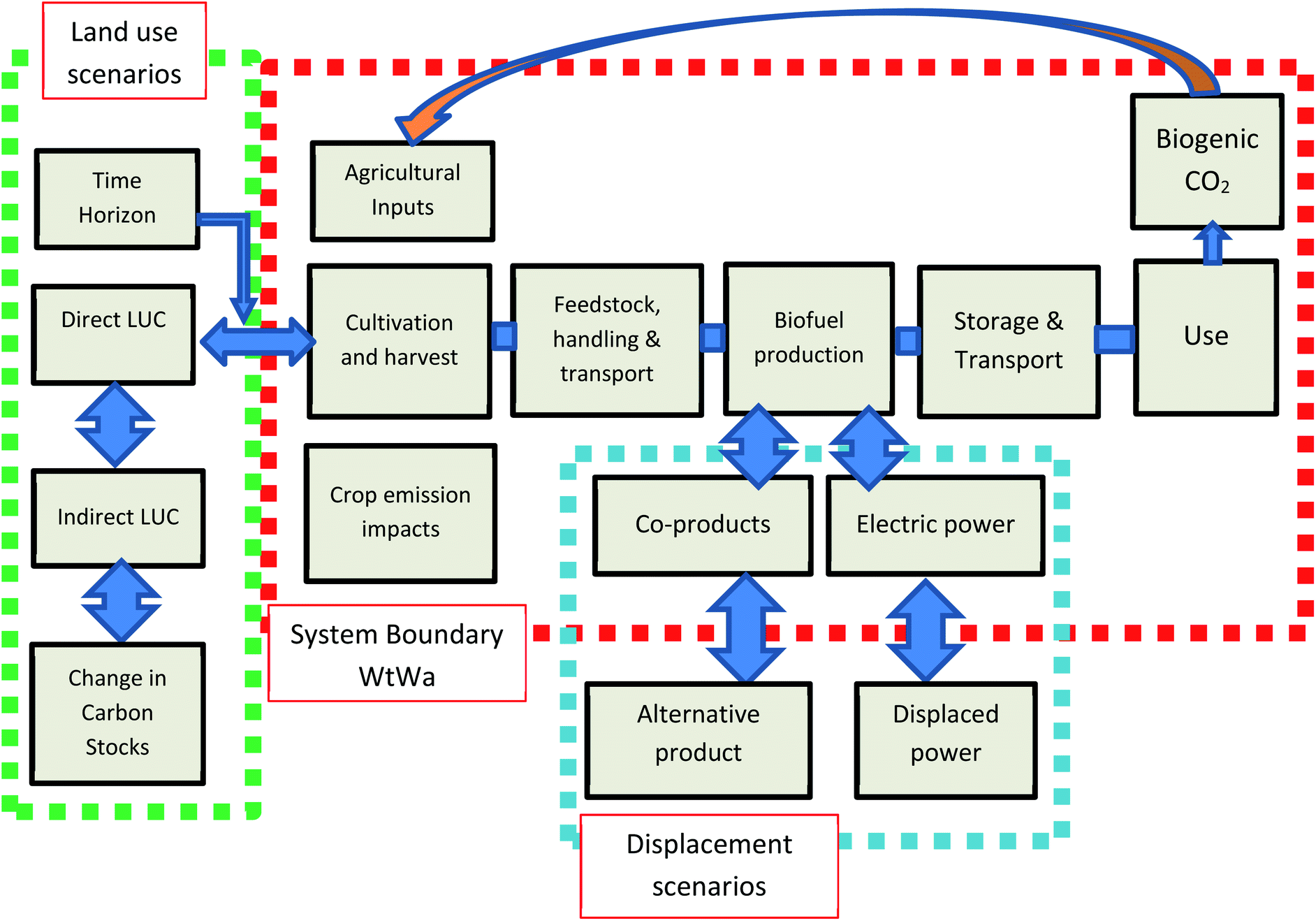
One of the contested debates in terms of applying LCA to AAF fuels is the setting of the system boundary.²² In Fig. 1, LCA features four typical boundary settings when applied to aviation fuel. The first is Well-to-Wake (WtWa) in the blue box and covers the full lifecycle of the fuel pathway from extraction to combustion of the fuel. Well-to-Pump (WtP) includes every step excluding combustion in the red box. The third boundary focus is Well-to-Gate (WtG) and an example can be seen in the green box. The final boundary configuration is Gate-to-Gate (GtG) in the orange box. The system boundaries cause significant uncertainty when performing comparisons with the rest of the LCA literature.² Across the system boundary, allocation is performed in order to partition environmental burdens of products or functions that are involved in or at least share the same process.² The allocation procedure (see Section 2.2) is primarily carried out through one of four ways, namely mass,⁴ displacement (system expansion), energy and economic (market) partitions. Implementation remains difficult with the methods interpreting results in different frames relating to the function of that specific method. Applying an attributional LCA to the WtP process boundary is straightforward; estimating the emissions from combustion is complex due to relative efficiencies of different types of aircraft in operation as well as distances covered. For example, long-haul aircraft are efficient over long distances such as transcontinental flights, while they are less so over short-term flights such as inter-city “hops” due to complex manoeuvring and power adjustment. Such studies are out of scope for this review but are readily available.^23–27

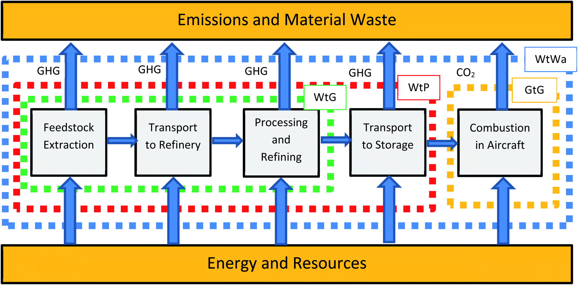Fig. 1 LCA system boundary analysis of a generic aviation fuel pathway. WtWa = well-to-wake; WtP = well-to-pump; WtG = well-to-gate; GtG = gate-to-gate.

This review aims to benchmark currently available studies on AAFs (2008–2018) and so aims to consolidate the work that was started in other review papers.^28–38 The focus of the review includes an analysis of the types of LCA performed, the process pathways, feedstocks and uncertainty associated with LCA. It also identifies what processes negatively influence upstream/embedded emissions and assists in the identification of which combination of processes and feedstock's provide the most optimal emission reduction.³⁹

Section 2 illustrates current regulatory policy and the general data requirements for AAF research, including key LCA tools (software and algorithms) and their terminologies. Section 3 introduces and describes the current AAF fuel technologies available, considering all feedstocks and process pathways as well as their commercial readiness. Section 4 critically evaluates the 37 LCA studies in terms of their results and trends. The distribution of conventional jet A1 is compared across the literature, since significant variation also exists with this baseline. Availability and scaling issues of each process is explored, as well as the uncertainty and distribution of the results. Finally, Section 5 provides a short prospective, highlighting available fuels that have not been assessed by LCA to produce aviation fuels as well as future work that discusses new technologies that require either modification of the existing aircraft fleet or the creation of entirely new aircraft to support such future pathways. The conclusions then close the paper.

2. Approaches, data requirements and resources

This section discusses the regulatory and general assumptions when configuring LCA. It explores policy, key LCA terminologies for assessing AAF, product allocation methods that have been applied and the role of the functional unit and system boundaries. Finally, LCA databases and tools are also explored and discussed.

2.1 LCA configurations for aviation fuel

2.1.1 Attributional and consequential. LCA can be grouped into two different categories – attributional and consequential studies.^6,40,41 Attributional applies sustainability parameters to a specific AAF pathway. Total impacts of the separate processes to produce aviation fuel can be easily summed, however indirect impacts from the refinery cannot be simulated and the system boundary is fixed on the product supply chain only. Direct environmental effects from input are included as well as the output i.e. combustion of the fuel.

Consequential LCA on the other hand allows the system boundary to include both direct and indirect effects of the production system with the realisation that the production is part of a larger system that can adjust its behaviour in response to the adjustments in production – essentially simulating cause and effect dynamics.^42–45 Additional environmental effects can be captured due to the ability to capture the dynamics of the system over time.

2.1.2 The functional unit (FU) and system boundary. The functional unit (FU) lies at the centre of all LCA studies,⁴⁶ providing normalisation metrics for the liquid fuel products. It is a common rule that the LCA should closely relate to the functions of the “product” as opposed to the physical or tangible product which is why an energy based FU is normalised based on one embodied MJ of its product and performed for the 37 studies with either g CO₂e per MJ or kg CO₂e per GJ.^47,48 The FU differs between product categories based upon the type of product that is being used and it should be able to compare across multiple different products. The FU differs between allocation and consequential methods. For allocation, the unit is fixed based upon the specified allocation parameters within a specific timeframe. For consequential decision making, the scale of the consequence may influence how the size of the functional unit is defined.

2.1.3 Time horizon. Most linear LCA studies do not consider time, and this of course causes considerable confusion. In order to be as realistic as possible, emission timing should be taken into account in order for the results to become more accurate.^15,49 For example, as new technologies emerge that are cleaner and more stable, this will have an impact on the LCA results. Ideally, the time horizon should equal the project lifespan.¹⁵ There is no clear quantitative method that is currently available that allows the selection of this value. The RFS2 analysis of land use emissions aimed to set fuel production to a time horizon of 30 years with the current yields being retained. The standard time horizon of 100 years which relates to the GWP potentials was also taken into account in all of the studies, however, serious challenges are present with such approaches. The first issue is that using the standard 100 year assessment period is suggestive of GHG emissions being passed on to future generations and there is an argument that the 20 year timeline should be implemented also for comparison purposes. Also, relying on GWP does not necessarily represent the true environmental impact or even the burden of cost. AAF projects may either fail quickly freeing up land for other applications or some biofuel projects may actually persist for much longer periods of time. Also, CO₂ sequestration on land addresses other challenges. One example of a time specific approach was introduced as a time shock value as opposed to spreading such environmental burdens equally throughout the selected time boundary⁵⁰ with the single impact being higher than the amortized value.⁵¹

2.1.4 Process efficiency. The process efficiency of the various pathways is dependent on the types of technology being used, and therefore, will determine the balance of emissions versus the production of fuel. Refinery process efficiency is also of primary interest in most studies. This can be expressed as an overall energy efficiency ratio (1):

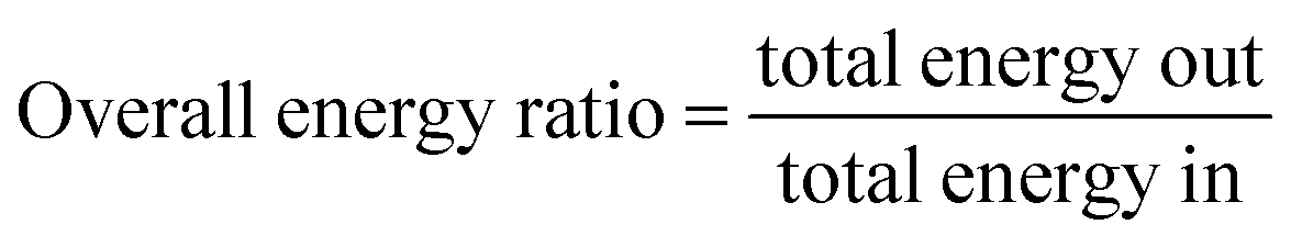
A process pathway energy ratio can be estimated by calculating the overall energy ratio (i.e., total energy in) to produce 1 MJ of jet fuel (i.e. total energy out). The amount of energy that is feeding into the system is derived from energy that is fed into the pathway in addition to all primary process requirements (electricity grid etc.). Process energy accounts for everything else and is dependent upon the efficiency of the overall process pathway. The overall energy ratio can be expressed by (2) as:

2.2 LCA allocation methods

As described earlier in Section 1, several allocation methods are available when comparing the LCA of AAFs. The most common include: (1) energy allocation;⁴ (2) mass allocation;⁵² (3) market or economic allocation^47,52 and (4) displacement, also known as system expansion or substitution.⁵³ Using only one of these methods can produce drastically different LCA results, and therefore, care must be taken when deciding on which allocation method should be used. Fig. 2 illustrates the type of allocation methods that have been applied to AAF LCA studies.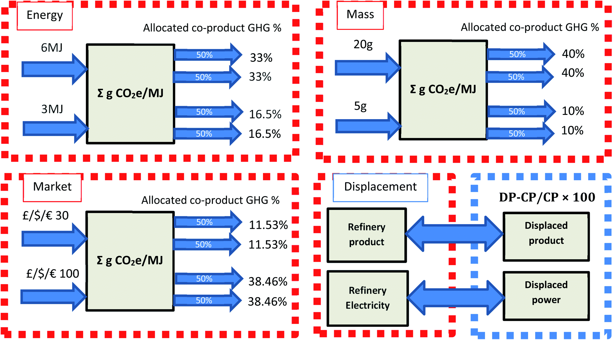

Fig. 2 Comparison of allocation methods applied to fictional alternative aviation fuel co-products produced at a generic refinery using dual feedstocks as input. The functional unit is represented by the central box for energy, mass and market allocation methods. The allocated co-product GHG% illustrates the change in emissions based upon the allocation method adopted. Note that the feedstocks and co-products are the same, only the allocation methods change, impacting the distribution of GHG results across different co-products.

2.2.1 Energy allocation. Energy based allocation aims to assess the LCA performance of a process pathway by allocating results based upon the energy content of a feedstock.^2,54,55 It is a requirement of the EU renewable energy directive.⁵⁶ Just like mass allocation, it is easy to apply and is probably the most relevant method to employ when assessing AAF technologies due to the variable energy content of feedstocks. Most of the EU literature uses the Lower Heating Value (LHV) for pre-production, while North America uses the Higher Heating Value (HHV) which includes the latent heat of water vaporization for post-production to determine energy content, which is proportional to the functional unit. All of the co-products that are produced for the final production of AAF can be used as energy sources, and therefore, it is logical to use this approach.⁴⁷

2.2.2 Mass allocation. Mass allocation is probably the simplest to perform, since it allocates emissions based upon co-product mass.⁵² This technique appears to be the most useful when co-product quantity is small compared with the aviation fuel fraction. In addition, it is preferred if a co-product substitute cannot be found that displacement/system expansion should be applied.⁴⁷ Other perspectives indicate mass allocation in liquid fuels which makes it difficult to compare technologies without first declaring their energy content, unless the co-products are displaced on a physical/mass basis.

2.2.3 Market allocation. Market value allocation offers both a fixed and non-linear approach, as the parameters may not be constants, but could consist of marginal data which can be forecasted through time.^48,57 Emissions and energy are allocated to the main supplier of the production of AAF based upon market dynamics driving the production.⁵⁸ If production from aviation fuels is being increased through demand, the price of the fuel also rises due to such demand. The monetary value of co-products falls as their additional supply increases resulting in a higher allocation of emissions to the main product and a reduced level of allocation to the co-products.

In effect, the aviation fuel product i.e. kerosene becomes the driving force of the AAF production pathway as well as its final emissions.⁵⁹ Unfortunately, it can be difficult to accurately measure market stability over time, which may introduce additional uncertainty such as fluctuations in oil price.^60–62

2.2.4 Displacement. Displacement is necessary in order to conform with the U.S. renewable fuel standard⁶³ and is the most logical choice for allocating the emissions and energy of AAF process pathways and feedstock's. It determines benefits from its co-products compared with conventional aviation fuels and credits them to the specified fuel product (known as discounting). For example, if industrially sourced CO₂ was considered as a feedstock, the avoided venting from the production source would be applied to the quantity of CO₂ that was processed in the aviation fuel production plant, effectively discounting its quantity from the atmosphere. This can be seen in Fig. 2, where refinery co-products and electricity production are being displaced with the business as usual case. Key difficulties for this type of method include finding an appropriate product which can be displaced, assessing the environmental burden and eventually finalising the appropriate displacement ratio.⁶⁴ There is also a considerable misunderstanding of how land use change emissions should be quantified, particularly first generation biomass feedstocks that are also produced as a food source e.g., soybeans and rapeseed featuring particularly large food-based markets.

As Fig. 2 illustrates, although the results can be different, there is no specific right or wrong approach to implementing product allocation methods, however, it is proving important (and perhaps necessary) to perform a comparative analysis using multiple allocation methods based upon the number of distinct scenarios. The type of feedstocks that are under scrutiny must be carried out on an independent basis due to the uniqueness of the feedstock and how they affect the process pathway once again highlighting the deviation of results in Fig. 2. The development of rulesets and guidance for assisting AAF modellers with applying the four allocation methods is currently ongoing.^22,56

2.3 Regulations, guidelines and accounting standards

Table 1 highlights 18 distinct regulatory approaches that are either actively engaged with assessing the performance of AAFs or possess the potential to do so. A variety of policies and frameworks exist in order to assess transportation fuels. Due to the similarity of their methodologies, it is possible that they could also be applied to the governance of the aviation industry.

Table 1 Regulations, guidelines and accounting standards influencing alternative aviation production^a

Fuel programs	Region	Responsible parties	Allocation approach	Calculation tools
a LCFS = low carbon fuel standard; CORSIA = carbon offsetting and reduction scheme for international aviation; EISA = energy independence and security act; RFS2 = renewable fuel standard 2^nd amendment; European RED = renewable energy directive; European ETS = emissions trading scheme; RTFO = renewable transport fuel obligation; CSBP = council for sustainable biomass production; GBEP = global biomass energy partnership; ISCC = international sustainability and carbon certification association; ISO = international standards organisation; RSB = roundtable for sustainable biomaterials; RSPO = roundtable for sustainable palm oil; RTSS = roundtable on responsible soy; EPD = environmental product declaration; PCR = product category rules; PAS = publically available specification.
Government regulations
California LCFS	California	Transportation fuel providers	Attributional, displacement	CA-GREET, GTAP
CORSIA	International	Flight operator and airline	Attributional, energy	GREET, E3
EISA section 526	U.S.	Federal agency fuel procurers i.e. Department of defence	Attributional	GREET
RFS2		U.S. fuel producers	Consequential, displacement
European RED	European Union	Fuel suppliers	Attributional, energy	Biograce
European ETS		European Union Industry (aviation to be included)	Non-specific	Non-specific
RTFO	United Kingdom	Fuel suppliers	Attributional	Default calculations
Sustainability guidelines
Bonsucro	International	Sugarcane producers	Non-specific	Non-specific
CSBP		Biomass and biofuel producers
GBEP		Biofuel analysts and policy makers
ISCC		Biofuel producers	Attributional, energy	ISCC GHG emission calculation
ISO 14040, 14044		Lifecycle assessment studies	Non-specific	Non-specific
RSB		Biofuel and biomaterial producers	Attributional, market	RSB greenhouse gas tool
RSPO		Palm oil producers	Non-specific	Non-specific
RTRS		Soy oil producers
Environmental accounting
EPD/PCR	International	Products with environmental declaration	Various	Various
ISO 14025
PAS 2050	United Kingdom

---

2.3.1 Government-based programs. A total of 7 government-based programs (Table 1) are currently in operation. These are the California low carbon fuel standard (LCFS),⁶⁵ the Carbon Offsetting and Reduction Scheme for International Aviation (CORSIA),⁶⁶ the U.S. Energy Independence and Security Act (EISA),⁶⁷ the U.S. renewable fuel standard (RFS2),⁶⁸ the European Renewable Energy Directive (RED)⁶⁹ and the Renewable Transport Fuel obligation (RTFO).⁷⁰

All support the assessment of GHG emissions and energy requirements, but they do not support other environmental criteria. When assessing their methodologies, they can be narrowed down to three key points. The first consists of co-product allocation methods and if displacement (Section 2.2.4) is being used across the system boundary. The second is double counting of co-products within the system boundary, which can lead to inaccurate conclusions in terms of environmental results. The third is the incorporation of land use impacts, which can be both direct and indirect, and depends on the type of associated feedstock. The choice of either consequential or attributional LCA causes different interpretations in terms of how the system boundary behaves. Finally, the default values for the regulatory frameworks may be different, and can therefore cause similarly performing feedstock pathways to behave differently. As an example, a pathway that produces surplus electricity, the RFS2 standard assigns emission-based credits depending upon the amount of surplus available.

Regulations have various accounting requirements for energy production, which can have implications on the emissions credit attribution. The LFS standard in Table 1 for example incorporates a regional grid mix. Under the RED framework, the emissions credit is fixed to the feedstock that was used to produce the electricity; therefore the assigned credit would be much lower as opposed to comparing directly with the regional grid mix which is naturally more emission intensive. In terms of more established standards such as the RFS2 and RED, it may be worthwhile in the future to harmonise the sustainability requirements for fuel production. This is because some pathways may accept a certain type of fuel by one regulatory body but would not be sufficient for another based on calculation methods, differences in GHG targets and land use requirements, which currently can act as barriers to implementation.

2.3.2 Voluntary based standards and independent bodies. Table 1 also illustrates a number of contrasting voluntary based programs consisting of independently run regulatory bodies and institutions that aim to standardise, promote and invest in improvements for sustainable aviation and similar industries. Such bodies emphasize and target specific sustainability characteristics and differ greatly between regional focus, feedstock scope and scale. For example, Bonsucro (UK)⁷¹ focuses on sugarcane feedstocks as well as its producers, however they do not feature or apply a specific LCA methodology to carry this out. Instead, they set mandatory targets of <24 g CO₂e per MJ of fuel-based emissions in order for mills and farms to remain certified. This target is much lower than the EU renewable energy standard (RED) which requires all fuels to be between <54.4–33.5 g CO₂e per MJ depending on whether installations were open before or beyond 5^th October, 2015. On the other hand, the Roundtable on Sustainable Biomaterials (RSB)⁷² focuses on all feedstocks and process pathways and features very distinct methodological requirements in the form of an attributional LCA assisted with data that is taken from various data sources such as Biograce.⁷³ In addition to small scale standards such as Bonsucro and RSB, the International Sustainability and Carbon Certification (ISCC)⁷⁴ and Council for Sustainable Biomass Production (CSBP) offers certification standards and guidelines for biomass derived fuels.

2.3.3 Environmental accounting standards. Supporting the regulatory bodies and governmental programs in Table 1 are three environmental accounting standards, which are designed to give guidance on environmental product declarations. The Public Available Specification (PAS 2050)⁷⁵ was created by the British Standards Institution in an attempt to standardize the methodology that is used in LCA and is based upon standards that have been developed by IPCC and ISO. Hence, it is designed to support consistency and step-by-step guidance on how to create an LCA for any product. In comparison between these two, system boundaries and functional units vary between the different products, however, PAS 2050 focuses on GHG emissions only compared with EPD's multiple environmental criteria. With the exception of ISO 14040, the basis for their guidelines consists of completely different standards. While PAS 2050 has a detailed LCA methodology drawn out, a Product Category Rule (PCR) is required which may lead to a long and difficult certification process. ISO 14025 (ref. 76) is designed to assess the requirements for designing EPD guidelines which is why it has been included in Table 1.

2.4 Databases and tools applied to alternative jet fuels

A variety of commercially available and free LCA software is available for analysing current AAF production pathways and simulations. In this section, we review seven commonly used approaches.

2.4.1 GREET. The GREET (Greenhouse gas Regulated Emissions and Energy use in Transportation) is an LCA tool which was developed by the Argonne National Laboratory, U.S. It is considered to be the most popular tool when assessing the LCA of AAFs.^47,77,78 Data from GREET is based mainly on U.S. sources and parameters (U.S. electricity generation mix via the U.S. Environmental Protection Agency's e-grid database, U.S. industrial statistics, U.S. transportation modes and distances⁷⁹). GREET has been credited by the Society of Automotive Engineers as the gold standard for WtWa analyses of vehicles and fuel systems. Since its creation, the U.S. government and industry have relied on the GREET model. Argonne's own simulations using ASPEN plus software for engineering processes, Autonomie simulations for vehicle fuel consumption and EPA MOVES modelling of vehicle emissions also use the GREET model. In terms of AAFs, a few studies have contributed to the refinement of the GREET database, such as Elgowainy et al.⁷⁸ and studies by the Massachusetts Institute of Technology (MIT).^{24,47,80–82}

2.4.2 Biograce. Biograce is a model that was developed by Intelligent Energy Europe.⁸³ The software follows the regulations of the EU RED (as described earlier in Table 1). It features two different scales in the form of general or country specific (i.e. Germany, Spain and Netherlands etc.). The functional units are derived from the European Commission's Joint Research Centre (JRC). It is capable of providing over 15 different biofuel pathways and allows for auditing. Co-products are allocated using the energy allocation method, therefore GHG emissions are partitioned using only this method, providing less flexibility compared to some of the other models currently available. However, Biograce can be updated through importing external LCI data. It does not calculate other impacts beyond CO₂e which is one of the major issues with the LCA aviation fuel literature.

2.4.3 ALCEmB (assessment of life cycle emissions of biofuels). ALCEmB is a lifecycle GHG model which is specifically created in order to assess biofuels and has been proposed by Lokesh et al.^84,85 GHG emissions are allocated to bio-SPKs from WtWa LCA configurations. ALCEmB adapts the process pathway conditions as well as the selected feedstocks in order to predict combustion emissions (see Section 4.4). In previous studies, it was assumed that combustion emissions were definite. Biomass credits are predicted via a special chemical algorithm determining hydrocarbon chemistry and constantly updated tracking of the carbon cycle. Water consumption is given a linear relationship in line with carbon intensity and specific engine configurations of aircraft and its systems are investigated. The core system boundaries of the ALCEmB tool is applied from the cultivation of biomass (representing the well/cradle) through to the combustion of the fuel product in the engine producing wake emissions (representing the grave). The tool primarily uses energy-based allocation as the core baseline scenario. Fuel specific systems are quantified through a specific module in addition to operational emissions. A fluid property library that contains several parameters for the aviation fuels is relative to temperature, fuel air ratio and pressure.⁸⁶

2.4.4 TLCAM (Tsinghua University LCA model). The Tsinghua University LCA Model or TLCAM was created to simulate the standard parameters of China's transport network and includes an LCA suite.⁸⁷ Most of the key transport modes are covered, as well as the two different versions of sustainable energy, which are utilised after data extraction in addition to the transportation only function. The indirect energy and the impacts of GHG emissions are assessed in detail so that descriptions of the environmental burden and energy requirements for the secondary energy pathways are shown in China.

2.4.5 NETL LCA tools. NETL LCA are a set of tools that were created by the National Energy Technology Laboratory (NETL) who assists in the support and implementation of LCA models for AAF production. They consist of the following models and programs. The NETL Fischer–Tropsch (FTL) black box model allows the user to enter different compositions of syngas with the expected output being displayed. The assumptions assume 50 000 bbl per day. Key outputs are CO₂ emissions, mass flows, required syngas input and the export of electricity from the facility. The coal and biomass GHG optimisation tool performs scenario analysis to optimise the performance of GHGs under various coal and biomass to liquids (CBTL) configurations through three different coal types (Montana Rosebud sub-bituminous coal, Illinois No. 6 bituminous coal or North Dakota Lignite).

2.4.6 GHGenius. GHGenius is an LCA tool based on transportation fuels⁸⁸ and features a variety of different biofuel feedstocks and process pathways. It is capable of analysing contaminants associated with the production of the 1^st generation of AAF fuels such as hydro processed fatty acids (HEFA)-based feedstocks. The tool was originally specific to Canada and used by Natural Resources Canada, but GHGenius can also calculate results for several other locations including India, Mexico and the U.S.⁸⁹. The three key GHGs are included in this model (i.e. CO₂, CH₄ and N₂O) as well as CFC-12 and HFC-134a and criteria pollutants. This model is a lot more complex than traditional LCA models and includes around 20 different regions and soil types, in addition to indirect GHG calculations as well as a non-linear simulation of the atmosphere. Over 200 feedstock pathways exist that focus on fuel, pathways and vehicles, however they do not measure the jet fuel pathway, as the focus is on ground transportation.

2.4.7 SimaPro and Ecoinvent. SimaPro (v8.5.2) is one of the most popular LCA software suites globally and includes the Ecoinvent database (v3.6).⁹⁰ Other databases that are included with SimaPro include the US Lifecycle Inventory database, Industry data 2.0, EU Danish input–output and the European Life Cycle Database (ELCD). As good background data is important, specifically in LCA, practitioners mainly use LCI databases, such as Ecoinvent, which can be considered to be one of the largest, most transparent and most fully-equipped unit-process LCI databases internationally. The most recent version, Version 3.5, provided several important methodological and technological improvements, as well as a high number of extensive and revised datasets.

3. Current pathways and feedstocks

The seven pathways that form the core AAF LCA literature consist of: Hydroprocessed Renewable Jet fuel (HRJ), also known as Hydroprocessed Esters and Fatty Acids (HEFA); pyrolysis (Hydrotreated Depolymerized Cellulosic Jet (HDCJ)); Fischer–Tropsch (FT); Catalytic Hydrothermolysis (CH), referred to as Hydrothermal Liquefaction (HTL) in this paper; Alcohol-to-Jet (ATJ); Sugar to Jet (STJ), also referred to as Direct Sugar to Hydrocarbons (DSHC), and Aqueous Phase Processing (APP) which can be considered as a secondary pathway to STJ. Fig. 3 illustrates the Commercial Aviation Alternative Fuels Initiative (CAAFI) Fuel Readiness (FRL) scale, measuring technological maturity for certification and commercial use.⁸³ FRL 1 in the CAAFI FRL scale indicates that basic principles have been observed and reported indicating that the feedstock and process principles have been identified. FRL 2 indicates that a technology concept has been formulated and a complete record of the feedstock process has been identified. FRL 3 is the proof of concept, which can be attributed to lab scale experiments that have validated the approach. An energy balance has also been undertaken and basic fuel properties have been validated. The fuel quantity that is to be prepared at this stage is 0.13 US gallons (500 ml). FRL 4 is divided into two parts, preliminary, technical and evaluation.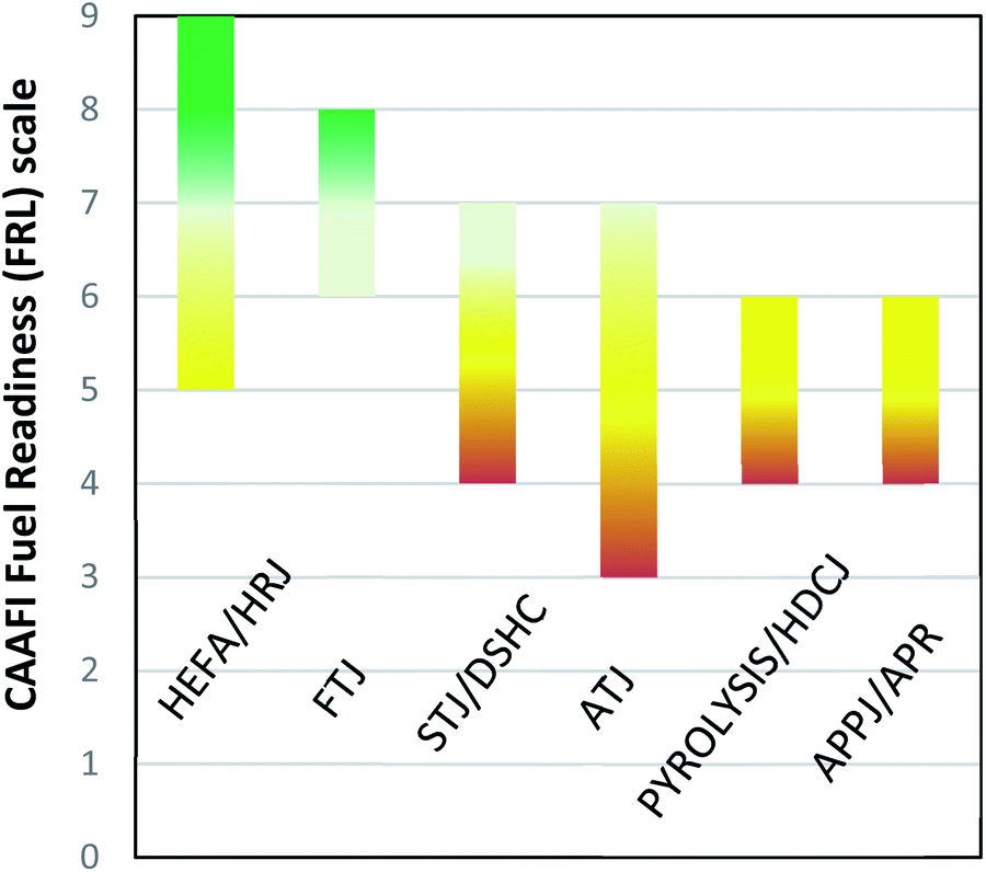

Fig. 3 CAAFI fuel readiness scale.⁹¹ HEFA = hydroprocessed esters and fatty acids; FTJ = Fischer–Tropsch; STJ/DSHC = sugar-to-jet/direct sugar to hydrocarbons; ATJ = alcohol-to-jet; HDCJ = hydrotreated depolymerized cellulosic jet; APPJ/APR = aqueous phase processing/aqueous phase reforming. Note that HTL does not yet have an FRL level.

System performance and integration studies are carried out and entry criteria/specification properties are evaluated. At this stage 10 US gallons (37.8 litres) of fuel are produced and given rigorous performance tests. According to Fig. 3, all of the pathways of the core LCA literature in this paper have reached FRL 5 dependent on pathway configuration which entails process validation and consists of gradual upscaling to an operational pilot plant. The quantity of fuel produced can be between 80 US gallons (302.8 litres) to 225 000 US gallons (851 715 litres). At FRL 6, a full-scale technical evaluation is conducted which includes fitness, fuel properties, rig testing and engine testing. The same quantities of fuel are produced here just as in FRL 5. FRL 7 provides the approval of fuel in a set of international standards. FRL 8 provides commercial and business model approval and a GHG assessment is carried out of the refinery using standard LCA techniques. At FRL 9 the commercial plant is fully operational.

3.1 Available pathways

3.1.1 HEFA/HRJ pathway. Hydroprocessed ester and fatty acids (HEFA/HRJ) according to Fig. 3, has a CAAFI FRL of between 5–9 depending on the feedstock and is one of the certified process pathways currently available for trials that are being carried out by major airlines.^{31,47,81,92–94}Fig. 4(a) illustrates the steps to produce aviation fuel from a WtP system boundary. Biomass is first harvested and transported to the refinery where the feedstock's molecules (consisting mostly of triglycerides in addition to fatty acids) are hydrogenated and isomerized in order to produce long chain hydrocarbons within a desired carbon length.^94–97 The most common feedstocks for this specific process include any form of oil and fats from both plants and animals including vegetable oils.

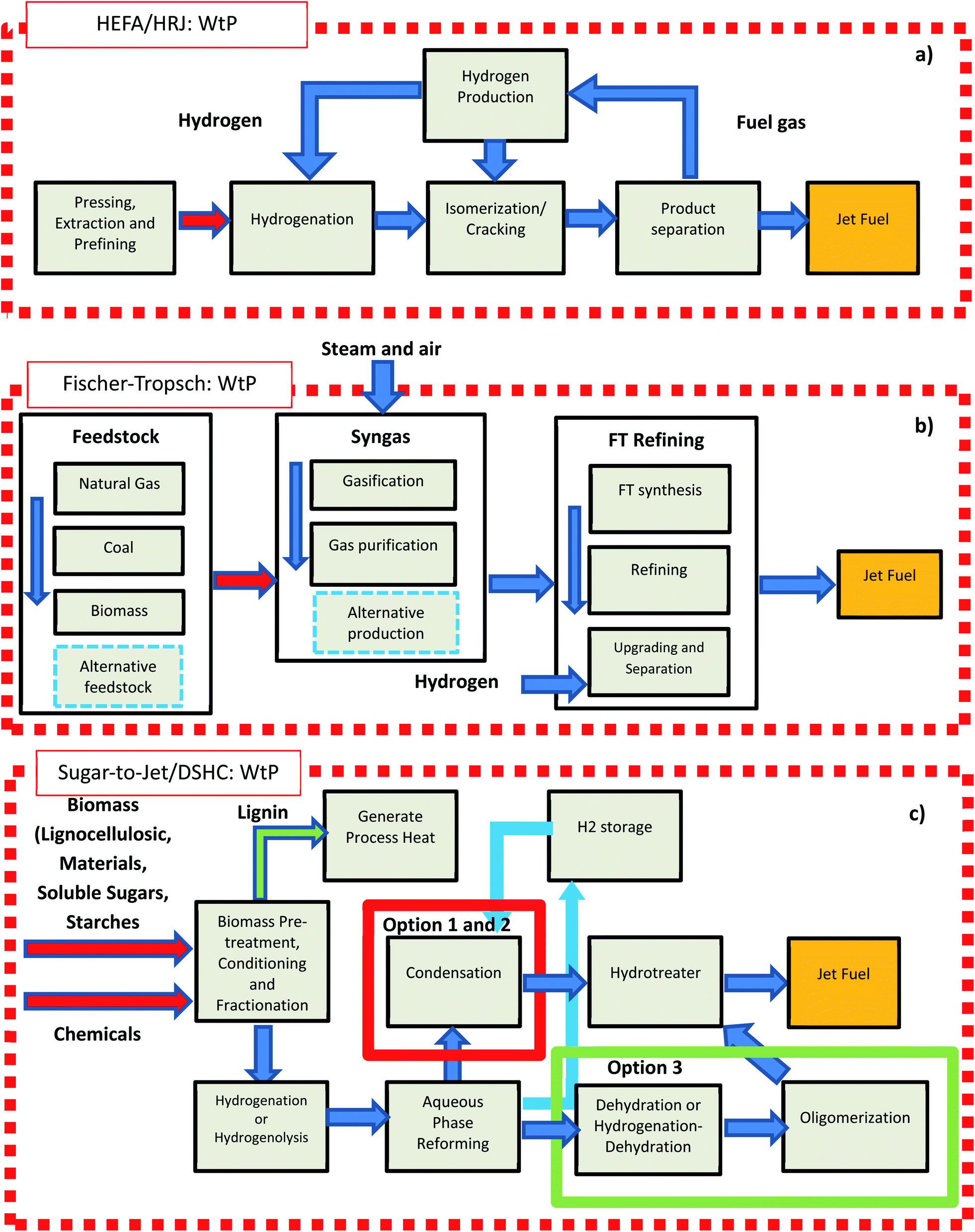Fig. 4 Overview of (a) HEFA/HRJ; (b) Fischer–Tropsch and (c) sugar-to jet. Red arrows indicate transportation emissions would be included at this specific phase of the process.

3.1.2 Fischer–Tropsch (FTJ) pathways. Fischer–Tropsch (FT) is a proven and well established pathway which produces aviation fuel by taking syngas as an input in addition to a number of other co-products. It was established in 1925 by the two German scientists Franz Fischer and Hans Tropsch.^98–101 According to the CAAFI fuel readiness scale (Fig. 3), FT has an FRL of between 6–8.⁹¹ FT is usually twinned with syngas production from gasification¹⁰² and has already been well established for over 80 years.¹⁰³ Depending on the configuration, the FRL level aims to make a decision on the type of feedstock to use for full commercial production. Unlike crude oil which can be synthesised to kerosene directly, coal requires the use of FT⁹⁹ (see Section 3.3.3). Fig. 4(b) illustrates such a configuration where syngas is produced from the gasification process. The gasifier then purifies the gas using a combination of steam and air to determine product composition. It is then sent to the FT refinery which refines, upgrades and separates the product. It is also possible that thermochemical conversion can be applied to produce syngas.¹⁰⁴ As well as other alternative syngas production approaches such as CO₂ electrolysis through direct air capture or source capture from industry (described in Section 5.1.2). Such approaches are represented in Fig. 4(b)via the alternative feedstock and production boxes with the dashed blue lines.

3.1.3 Sugar-to-jet (STJ) pathways. STJ involves the conversion of sugars to jet fuel^105–108 According to Fig. 3, STJ has a FRL rating of between 6 and 7 indicating that up to 225 000 US gallons (851 715 litres) can be produced as well as the establishment of a set of international standards.

According to the literature, there are two primary STJ pathways that exist. The first is based on catalytic upgrading of sugars and their intermediates to suitable hydrocarbons.¹⁰⁹ The second approach consists of the biological conversion of sugars and their intermediates to hydrocarbons.¹¹⁰ Significant research has been carried out into the fermentation of hydrocarbon fuel. Fig. 4(c) illustrates this process via the conversion of biomass into solubilized sugars. This process is typically carried out through the biomass pre-treatment phase and the appropriate enzymatic hydrolysis of biomass in order to create the C5 and C6 sugars. The second phase involves the transportation of purified hydrolysate to reforming reactors where carbohydrates are converted in the presence of hydrogen into polyhydric alcohols through hydrogenation. The hydrotreated product is then sent directly to the APR reactor where it is reacted with water over a catalyst between 450 to 575 K and pressures of 10 to 90 bar. Hydrogen is produced using the APR reactors. The types of feedstock that are available for sugar-to-jet tend to include lignocellulosic materials, soluble sugars and starches. According to the literature, there are three possible approaches to converting oxygenates during the reforming step into appropriate hydrocarbons¹¹¹ which include option 1: acid condensation, option 2: aldol condensation and option 3: dehydration or hydro-dehydration.

3.1.4 Alcohol-to-jet (ATJ) pathways. ATJ and its alternative term alcohol oligomerization is converted from a variety of different chemicals such as methanol, ethanol, butanol and a long chain of different fatty based alcohols.^112–116 According to Fig. 3, it has an FRL level of between 3 and 7 indicating significant deviations in the type of feedstock used as well as the pathway configuration. The quantity of fuel that can be produced is from lab scale 0.13 US gallons (500 ml) up to pre-commercial production volumes i.e. 225 000 US gallons (851 715 litres). In some cases an FRL level of 7 indicates ATJ features a set of international standards for full commercial use. Fig. 5(a) illustrates a typical ATP pathway taking methanol as an input where it is dehydrated and fractionated. After fractionation C₁–C₃ paraffin's are recycled to be dehydrated further. C₄ paraffins and olefins are fractionated into jet fuel. The main advantages of ATJ pathways include the potential of higher availability of feedstocks, i.e. sugar/starch and lignocellulosic biomass are abundant. In addition, the technological maturity of ATJ conversion is also high, particularly when using starches and sugar based feedstocks. Within the U.S., ethanol is added to a specific type of petrol i.e. E10. The amount of ethanol that was produced in the U.S. equalled 55.6 billion litres in 2015. The main advantages of ATJ pathways include the potential of higher availability of feedstocks, i.e. sugar/starch and lignocellulosic biomass are abundant. In addition, the technological maturity of ATJ conversion is also high (see Fig. 3), particularly when using starches and sugar based feedstocks. Within the U.S., ethanol is added to a specific type of petrol i.e. E10. The amount of ethanol that was produced in the U.S. equalled 55.6 billion litres in 2015. Gasoline equalled 553 billion litres (2015) although this is expected to decline due to increases in renewable energy shares.¹¹⁷ Through the 10% blend wall, the production of ethanol may supersede the consumption within the US E10 market, providing some additional approaches for ATJ technology growth.

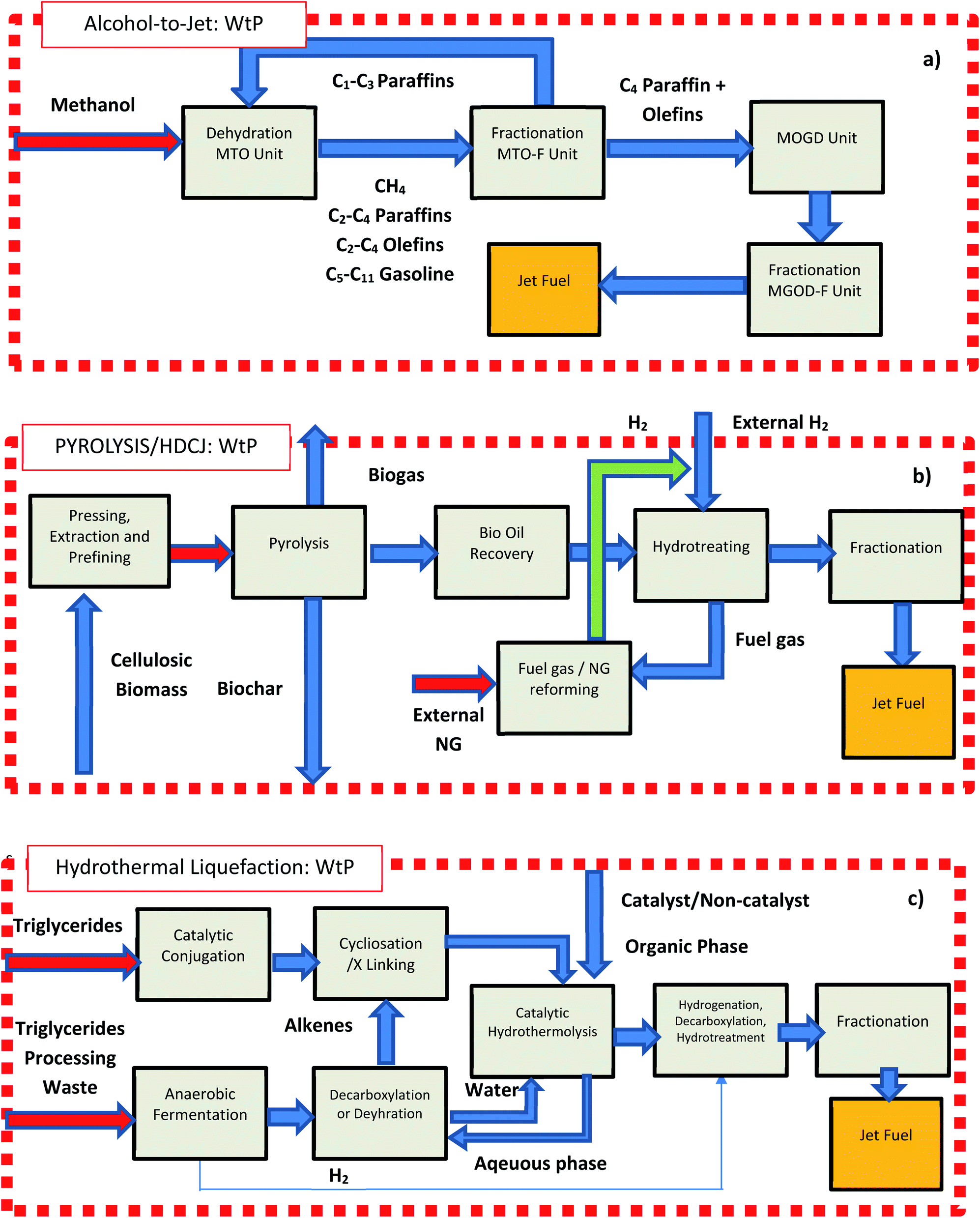Fig. 5 Overview of (a) alcohol-to-jet and (b) pyrolysis and (c) hydrothermal liquefaction pathways.

3.1.5 Pyrolysis/HDCJ. Pyrolysis is a process that aims to heat various forms of biomass without the use of oxygen through different process speeds.^{30,78,118,119} According to Fig. 3, pyrolysis has a FRL level of between four and six and produces pyrolysis gas, biochar and pyrolysis oil.¹¹¹ The pyrolysis pathway, also known as Hydrotreated Depolymerized Cellulosic Jet (HDCJ) can covert biomass into jet fuel although it currently has not been approved by ASTM. Like HEFA, the oils from the pyrolysis process undergo hydrotreatment in order to create the aviation fuel product.¹¹¹Fig. 5(b) illustrates the process pathway. Where the biomass is extracted and transported to the refinery. The next step involves pyrolysis of the feedstock where biogas is produced and diverted to be reused, possibly as a power or heat source. The bio oil is then recovered and then hydrotreated. Finally, fractionation occurs which produces the aviation fuel. The feedstocks that are most related to this pathway include corn stover, switchgrass, sugarcane bagasse, guinea grass, algae biomass and forest residue.⁷⁸

3.1.6 Aqueous phase processing (APP). Aqueous-phase processing (APP) or aqueous phase reforming is another approach synonymous with sugar-to-jet which converts cellulosic biomass thermochemically into AAF and co-products.^120–124 According to Fig. 3, they currently have an FRL level of between 4–6 indicating that system performance and integration studies are carried out and the potential quantity of jet fuel that can be produced at this stage is between 10 US gallons (37.8 litres) and 225 000 US gallons (851 715 litres). APP can produce hydrogen from biomass based oxygenated compound i.e. sugar and sugar alcohols. The potential for energy efficiency is significant as all of the reforming is carried out within the liquid phase hence it does not volatilize the water. Another benefit is that the water–gas shift reaction is favourable to the temperatures necessary for APP, therefore CO is minimized and decomposition is almost eliminated. Fig. 5(c) illustrates the aqueous phase reforming process via the conversion of biomass into solubilized sugars.

3.1.7 Hydrothermal liquefaction (HTL). HTL is a thermal depolymerisation process used to convert under moderate temperatures and high pressure wet biomass into crude like oil.^125–133Fig. 3 indicates an FRL of 4–6 indicating between 10 US gallons (37.8 litres) to 225 000 US gallons (851 715 litres) can be produced depending upon the pathway configuration and the technology that is used. According to Fig. 5(c), third generation feedstock's, i.e. algae and microalgae, tend to use HTL due to their high moisture content, but theoretically almost any type of biomass can be used in this process.³⁴ This process is carbon-neutral i.e. plant based biomass has carbon stored from photosynthesis and when it is exposed to HTL the carbon is released back into the atmosphere, albeit completely offset from the carbon that has been collected by that specific biomass type (stated earlier in Section 3.4). Although HTL and pyrolysis are indeed related, it needs to be considered that biomass with a high moisture content (algae and microalgae for example), can produce bio jet fuel which has a 2 : 1 energy density ratio than pyrolysis-based oil. Biomass within the pyrolysis process is dried in order to increase the yield. In addition, algae oil contains up to 80 wt% in terms of feedstock carbon content.

3.2 Current feedstocks

Table 3 illustrates the properties of the feedstock. Each of the feedstocks contain unique properties that can affect the partitioning of GHG emissions depending upon the allocation factor that is used (see Section 2.2). Such parameters that can effect LCA partitioning including mass based parameters such as weight and density (ρ) in addition to the chemical compositions (C, H, N, O, S). Energy based allocation can be affected by the calorific or lower heating value (LHV) in addition to the process efficiency of the pathway (see Section 2.1.4).

3.2.1 Conventional crude oil. Traditional jet A/A1 is a kerosene based feedstock with multiple components and feature a carbon chain length of C⁸–C¹⁶ manufactured from lamp oil.¹³⁴ The primary feedstock is extracted from crude oil that is recovered from below the surface after millions of years of fossil compression. Kerosene production has improved in terms of consistency and is evolving through changes in security of supply and safety criteria. The kerosene composition consists of aromatics and cycloparaffins or naphthenes. Paraffins and olefins are also included, albeit in small amounts.¹³⁵Table 3 indicates that aviation fuel has an average LHV of 43.2 kg MJ⁻¹i.e. 23.17 g MJ⁻¹. Carbon content is high as expected from crude oil (86.2%). Ultra-low sulphur jet fuel is regarded as the most common conventional pathway and includes hydrotreatment so that sulphur content is reduced to ∼5 ppm as indicated in Table 3.

3.2.2 Unconventional crude oil. Unconventional crude oil derives from a selection of different liquid sources, which include extra heavy oil, gas to liquids, other liquids and oil sands.^136–143 Such oils are extracted using different methods compared with the oil well method.¹⁴⁴ The two most dominant types of unconventional crude oil are oil sands and oil shale. Two of the largest reserves of unconventional crude oil are oil sands in Alberta (Canada) and oil shale embedded in the Green River formation in parts of Colorado, Utah and Wyoming (U.S.).¹⁴⁵ According to Table 2, the chemical composition of unconventional crude oil is similar to conventional crude.

Table 2 Overview of the LCA studies highlighting AAF feedstock properties and chemical compositions by the literature. VM = volatile matter; FC = fixed carbon; M = moisture content; LHV = lower heating value; ρ = density; C = carbon; S = sulphur; O = oxygen; H = hydrogen; N = nitrogen; Cl = chloride and A = ash yield

Feedstocks	AAF LCA studies	VM	FC	M	LHV	ρ	C	S	O	H	N	Cl	A
Conventional crude oil
Petroleum	Elgowainy et al.^156	No data available			43.2	0.8	86.2	3.0	1.0	12.5	0.6	No data available
	Wong^47							600
P ultra-low sulphur	Elgowainy et al.^156					0.7	86.0	11
	Vera-Morales and Schäfer^157				42.8	0.8	86.2 (ref. 47)	<0.1
	Wong^47				43.2	0.7	86.0	15
	Lokesh et al.^158				43.1	0.8	86.2 (ref. 47)	<0.1
Unconventional crude oil
Crude mixture	Elgowainy et al.^156	No data available			43.2	0.8	86.2	700	1.0	12.5	0.6	No data available
Oil sands	Vera-Morales and Schäfer^157				42.8			0.05
	Wong^47				43.2			600
Oil shale	Vera-Morales and Schäfer^157				42.8			0.05
	Wong^47				43.2			600
Coal
Coal (bituminous)	Wong^47	29.1	52.6	32.1	24.4	N/D	61.2	1.1	9.5	15.0	11.3	<0.1	15.2
	Skone et al.^159						63.75			5.0	1.3
	Vera-Morales and Schäfer^157				44.1	0.7	83.1	<0.1
Coal (U.S. average)	Stratton^77	30.8	43.9	5.5	22.7	N/D	59	1.7	13.6	5.2			19.8
Coal w/switchgrass	Kinsel^160	No data available			No data available
Coal w/switchgrass	Skone et al.^159
Coal w/forest residue	Elgowainy et al.^156
Coal w/switchgrass	Stratton^77				22.7	N/D	59	11k	N/D	N/D	N/D	N/D	N/D
Municipal solid waste
Municipal solid waste	Suresh^82	70.3	0.5	4.2	19.99	N/D	48.0	1.5	36.8	7.8	1.1	<0.1	<0.1
Natural gas
Natural gas	Elgowainy et al.^156	Not applicable			47.1 (ref. 47)	0.2 (ref. 47)	72.4	6.0 (ref. 47)	No data available
	Olcay et al.^161
	Vera-Morales and Schäfer^157				50	0.2 (ref. 47)		<0.1
	Wong^47				47.1	<0.1		6.0
Biomass
Algae and microalgae	Agusdinata^162	45.1	23.1	10.7	44.1 (ref. 127)	0.7	43.2	2.6	45.8	6.2	2.2	2.6	21.1
	Connelly et al.^127						52.0
	Elgowainy et al.^156						84.7
	Cox et al.^163						43.2
	Fortier et al.^164						78.7	<0.5
	Handler et al.^126				24.0		43.2	2.60
	Lokesh et al.^158				43.2			<0.1
	Ou et al.^165				44.1 (ref. 127)		50.0	2.6
	Guo et al.^166						43.2
	Vera-Morales and Schäfer^157
	Carter^80						78
Camelina	De Jong et al.^83	64.3	15.3	14.4	44.1 (ref. 158)		51.3	0.19 (ref. 158)	41.0	6.3	1.2	0.1	6.0
	Agusdinata^162
	Li and Mupondwa^167				44.0			<0.1
	Lokesh et al.^158				44.1
	Shonnard et al.^168
Canola	Ukaew^169	N/D	N/D	N/D	N/D		N/D	N/D	N/D	N/D	N/D	N/D	N/D
Corn (maize)	Han et al.^105	67.7	17.8	7.4	16.3 (ref. 77)		44.5	0.1	44.1	6.4	0.7	0.6	7.1
	De Jong et al.^83
	Staples et al.^170
	Han et al.^105
Corn stover	Agusdinata^162
	De Jong et al.^83
	Han et al.^105
	Stratton^77
Eucalyptus bark	Crossin^171	68.7	15.1	12.0	N/D		48.7	<0.1	45.3	5.7	0.3	0.2	4.2
Forest/woody residue	Agusdinata^162	57.4	12.2	26.4	15.4 (ref. 77)		51.4		41.9	6.1	0.5	<0.1	4.0
Forest residue	Elgowainy et al.^156	34.5	7.3	56.8	16.3		52.7	0.1	41.1	5.4	0.7		1.4
	De Jong et al.^83
	Ganguly et al.^172
	Pierobon et al.^173
	Stratton^77				15.4		51.7
	Wong^47				16.3
German substrate	Neuling and Kaltschmitt^116	N/D	N/D	N/D	N/D	N/D	N/D	N/D	N/D	N/D	N/D	N/D	N/D
Jatropha curcas	De Jong et al.^83	64.3	15.3	14.4	19.0	0.7	84.2	<0.1	41.0	6.3	1.2	0.1	6.0
	Stratton^77
	Bailis & Baka^174
Jatropha curcas	Lokesh et al.^158	N/D	N/D	N/D	44.3	N/D	N/D	N/D	N/D	N/D	N/D	N/D	N/D
	Neuling and Kaltschmitt^116				N/D
Manure
Naphtha	Stratton^77	64.3	15.3	14.4	44.4	0.7	51.3	<0.1	41.0	6.3	1.2	0.1	6.0
Pennycress	Fan et al.^175				36.6
Pongamia	Cox et al.^163				N/D
Palm	Neuling and Kaltschmitt^116	N/D	N/D	N/D	N/D		N/D	N/D	N/D	N/D	N/D	N/D	N/D
	Wong^47	46.3	12.0	36.4	44.0		51.0	0.3	40.1	6.6	1.5	N/D	5.3
Poplar	De Jong et al.^83	79.7	11.5	6.8	N/D		51.6	<0.1	41.7	6.1	0.6	N/D	2.0
	Budsberg et al.^176
Rapeseed	Stratton^77	70.7	16.3	8.7			48.5	0.1	44.5	6.4	0.5	<0.1	4.3
Salicornia		64.3	15.3	14.4	16.3		51.3	<0.1	41.0	6.3	1.2	0.1	6.0
Soybean	Elgowainy et al.^156	69.6	19.0	16.3			84.7	0.1	46.9	6.7	0.9	N/D	5.1
	Wong^47						87.1
Sugarcane^177	Michailos^178	76.6	11.1	10.4	7.5		49.8	<0.1	43.9	6.0	0.2	<0.1	1.9
	De Jong et al.^83
	Moreira et al.^179
	Staples et al.^170
Switchgrass	Agusdinata^162	70.8	12.8	11.9	17.6		49.7	0.1	43.4	6.1	0.7		4.5
	Staples et al.^170
	Olcay et al.^161						47.0	0.1
	Stratton^77
Tallow	Seber et al.^81	61.7	12.4	2.5	N/D		57.3	20.8	8.0	12.2	1.69	0.87	23.4
Wheat grain	Neuling and Kaltschmitt^116	N/D	N/D	N/D			N/D	N/D	N/D	N/D	N/D	N/D	N/D
Wheat straw		67.2	16.3	10.1			49.4	0.17	43.6	6.1	0.7	0.61	6.4
Willow^177							49.8	0.06	43.4	6.1	0.6	0.01	1.4
	De Jong et al.^83	74.2	14.3
Wood (red maple)	Olcay et al.^161	70.1	17.8	8.4			45.4 (ref. 180)	0.11	41.3	6.2	0.4	N/D	3.7
Yellow grease^181	De Jong et al.^83	61.7	12.8	11.9	17.6 (ref. 77)		76.4	<0.1	11.2 (ref. 181)	12.2	N/D	N/D	N/D
	Seber et al.^81
Chemicals
Ethanol	Capaz et al.^182	N/D	N/D	N/D	N/D	N/D	N/D	N/D	N/D	N/D	N/D	N/D	N/D
	Olcay	N/A	N/A	N/A	N/A	N/A	N/A	N/A	N/A	N/A	N/A	N/A	N/A
Methanol		N/A	N/A	N/A	N/A	N/A	N/A	N/A	N/A	N/A	N/A	N/A	N/A
Seawater	Falter^104	N/A	N/A	N/A	N/A	N/A	N/A	N/A	N/A	N/A	N/A	N/A	N/A

---

Both oil and gas can be produced from shale using a method known as retorting.¹⁴⁶ The shale is heated in order to convert kerogen to liquid and gaseous hydrocarbons.¹⁴⁷ As with oil sands, surface and in situ methods can be utilised to extract the oil and the surface mining involves crushing and retorting in an above ground facility. The in situ process heats the oil shale while still underground so that it can be extracted and eventually transported to the surface. Surface retorting is the most emission intensive process as it operates at up to 750 °C.¹⁴⁸ Carbonate minerals decompose releasing CO₂ back into the atmosphere. Surface retorting damages land¹⁴⁹ and is considered controversial internationally, suggesting that the damage impact categories of an LCA would commonly indicate mass fouling of land to local ecosystems (Fig. 6).¹⁵⁰

Fig. 6 Conventional, ULS and unconventional jet fuel pathways.

3.2.3 Coal. Coal – another fossil fuel – can be considered as the first direct alternative to crude oil due in part to its relative historical abundance.^151–153 Unlike crude oil which can be synthesised to kerosene directly, coal requires the use of FTL⁹⁹ (see Section 2.3.2). Table 3 illustrates the general ash composition of bituminous and sub-bituminous coal, which is high in Al₂O₃ and SiO₂ compared to biomass and Municipal Solid Waste (MSW) but low on K₂O. In addition, U.S. averages are given from 37 samples. There are essentially two different approaches for producing coal through liquefaction: indirect¹⁵⁴ (current technology) and direct¹⁵⁵ (laboratory stage at time of publication). In the indirect process, the hydrocarbon chains are reduced through a decomposition process with reorganisation of the molecules to optimum production configurations.

Table 3 Elemental analysis of selected fossil and biomass feedstocks (adapted from ref. 177)

Feedstocks	SiO2	CaO	K2O	P2O5	Al2O3	MgO	Fe2O3	SO3	Na2O	TiO2	Sum	Mn (ppm)	Samples
Coal
Coal (bituminous)	56.1	4.9	1.6	0.2	24.8	1.5	6.6	2.1	0.7	1.1	100	511	22
Coal (sub-bituminous)	54.7	7.05	1.67	<0.1	22.8	2.14	5.30	4.07	1.09	1.00		509	N/D
Coal (U.S. average)	54.0	6.5	1.6	0.5	23.1	1.8	6.8	3.5	0.8	1.0		543	37
Biomass
Algae/microalgae	1.6	12.3	15.3	9.7	0.8	12.5	1.8	25.7	19.8	N/D	99.9	326	11
Corn stover	49.9	14.7	18.5	2.4	5.0	4.4	2.5	1.8	0.1	0.2	100	620	1
Eucalyptus bark	10.0	57.7	9.29	2.3	3.1	10.9	1.1	3.4	1.8	0.1		10 850
Forest residue	20.6	47.5	10.2	5.0	2.9	7.2	1.4	2.9	1.6	0.4		13 180	3
Forest/woody residue	53.1	11.6	4.8	1.3	12.6	3.0	6.2	1.9	4.4	0.5		N/D	2
Palm	63.2	9.0	9.0	2.8	4.5	3.8	3.9	2.8	0.8	0.2			1
Rapeseed	40.8	30.6	13.4	2.2	5.4	2.0	2.0	2.6	0.4			310	N/D
Switchgrass	66.2	10.2	9.6	3.9	2.2	4.7	1.3	0.8	0.5			N/D	3
Tallow	<0.1	41.2	3.1	40.9	2.3	1.3	0.2	4.2	6.4	<0.1		78	1
Wood (red maple)	8.9	67.3	7.0	0.7	3.9	6.59	1.43	1.99	1.76	0.12		5430	2
Municipal solid waste
Municipal solid waste	38.6	26.8	0.2	0.7	14.5	6.4	6.2	3.0	1.3	1.9	100.0	N/D	1

---

According to Table 2, the U.S. average of coal has an LHV of 22.7 kg MJ⁻¹. The direct process converts coal into liquids directly with no intermediate steps through breaking down the organic structure of coal with catalysts or solvents.

This procedure is typically carried out in an environment with high temperature and pressure. WtWa emissions of coal can vary sporadically depending upon technologies used and emission control mechanisms in place. Coal is the first feedstock that has been produced on a large scale as an AAF through Sasol's full synthetic jet fuel.¹⁸³ 50% of coal blends are carried out with standardised jet A-1 fuel.¹⁸⁴ Coal is the first feedstock that has been produced on a large scale as an AAF through Sasol's full synthetic jet fuel.¹⁸³ 50% of coal blends are carried out with standardised jet A-1 fuel.¹⁸⁴ Under DEF STAN 91-91, AAFs can be utilised in commercial flights through a maximum of 50% concentration as long as there is sufficient lubricity and 8% aromatics are present within the final product. These must all originate from the blending of petroleum.

However, most studies on coal feature LCA emissions exceeding the WtWa of conventional jet fuel. Coal can be gasified and is a process that directly precedes FT catalytic conversion.

3.2.4 Natural gas. NG is the third and final historically abundant fossil fuel. Synthetic oil and its production process from NG closely parallels coal liquefaction using the gasification/FTJ process pathway.¹⁸⁵ The only difference is that energy requirements are not as intensive compared to coal. Numerous studies for harnessing NG for aviation fuel have been carried out.^47,77,78,157 In addition, most studies report that the embedded emissions of using NG constitutes worse emissions than conventional jet fuel because of the high methane content which must be gasified in order to produce the syngas to produce the fuel (see Section 3.4).

3.2.5 Biomass. Biomass constitutes the majority of the LCA studies on AAF and features sporadically differing process pathways and results due to the wide variety of feedstocks and their compositions. Table 3 also illustrates that biomass, particularly algae, feature commonly high levels of moisture, Cl, K, Na, Mn in addition to trace elements¹⁷⁷ indicating that Biomass can be broken down into a variety of different categories and generations. The first generation conflicts with human food sources and industry.¹⁸⁶ Examples of first-generation biofuels include starch, sugar and vegetable oil. Fig. 7 illustrates an overview of the biomass system boundaries, highlighting how the LCA tends to be configured for biomass. In a typical full WtWa system boundary when assessing alternative aviation fuels, biogenic CO₂ uptake in biomass is in equilibrium with the combustion of CO₂ during flight, and the literature assumes that combustion emissions would typically be offset.⁴⁷ LUC scenarios tend to be added to the sensitivity analysis and consists of time horizon, direct LUC such as the physical planting and removal of biomass as well as the change in carbon stocks over time. Emissions are allocated based upon the cultivation of the land. Fertilizer for example can be emission intensive and will therefore increase the emission burden. Various displacement scenarios can take place which compares the product or co-products at the refinery with alternative products that have been avoided. This can either cause emissions to increase or decrease based upon the emission intensity of the product.

Fig. 7 Overview of biomass system boundaries and example scenarios.

The second generation of feedstocks attempts to avoid the conflict between human consumption and AAF production, and therefore, all second generation feedstocks are non-food based or are not traditionally consumed on a large scale.¹⁸⁷

Examples of second generation feedstocks include wood based crops and agricultural waste residues which are more difficult to extract.^2,32 Different process pathways are usually required for this type of feedstock although wood-based biomass can use conventional gasification/F–T synthesis.^188,189 Another argument for adopting second generation biofuels is the efficiency that they can be refined at, i.e. no waste compared with first generation biofuels.¹⁹⁰ Other feedstocks such as Municipal Solid Waste (MSW) contains a mixture of different substances containing refuse, food waste (considered to be the organic fraction) as described in Table 3 and commercial and industrial waste.^82,191 It is a promising feedstock as it has the potential to reduce land use and offset unsustainable disposal of rubbish into sensitive zones such as ocean and landfill and can offset waste management strategies. One of the biggest drawbacks to this feedstock is its high variability and non-uniform composition.

Table 2 illustrates an average approximation into what the potential chemical properties of MSW could be but it is for refuse only. For the production of jet fuel, MSW is processed using the gasification and FT combination

The third generation is derived around algae based feedstocks¹⁹² and their diversity is impressive. Algae can produce much more additional fuels than the previous generations by up to 10× the normal amount of some first and second generation biomass.¹⁹³ Unfortunately, the capital costs for this type of generation are the highest.¹⁹⁴ Algae or microalgae contains approximately 70% lipid content (dry weight) and present the capability to be nurtured in various wastewater streams, such as saline or brackish water and seawater near coasts resulting in reduced freshwater demand within LCA results.¹⁹⁵ Current efforts are on finding an ideal species of algae featuring high growth conditions and lipid content.

4. Evaluation of aviation fuel lifecycle results

This section focuses on a detailed analysis of all 37 currently published LCA studies of AAFs, supported by the wider renewable fuels literature. Table 4 illustrates a breakdown of all the LCA studies currently available. The LCA scope emphasizes whether the assessment incorporates a techno-economic assessment in addition to the environmental investigations. Out of the studies available, 15 (40%) contain some form of techno-economic assessment and interested readers can refer to these assessments here.^{80,81,104,116,157,160–162,169,170,178,196–198}

Table 4 Current LCA studies on jet fuel including LCA type, software, impact methods and characterisation factors. Uncertainty methods were also illustrated where available. LCA types may also include an economic component in the form of a techno-economic analysis. This is shown in the appropriate category. Note that we use displacement to also account for system expansion allocation methods

LCA studies	LCA scope	LCA type	LCA software/toolkit	Allocation method	Uncertainty methods
Wong^47	Environmental	Attrib/conseq.	GREET	Disp., energy, market, mass	High–low sensitivity pathways
Vera Morales and Shafer^157	Enviro/tech-eco.	Attributional	Custom	Market, mass	None
Stratton^77	Environmental	Attrib/conseq.	GREET	Disp., energy, market,	High–low sensitivity pathways
Bailis and Baka^174			SimaPro	Disp., energy, mass	Energy/mass based allocation
Kinsel^160	Enviro/tech-eco.	Attrib/conseq.	Eiolca.net	Market	None
Shonnard et al.^168	Environmental	Attributional	SimaPro v7.1	Disp., energy, mass	High–low sensitivity pathways
Skone et al.^159			NETL LCA tools		Probabilistic uncertainty
Agusdinata et al.^162	Enviro/tech-eco.	Consequential	Custom	Market
Handler et al.^126	Environmental	Attributional		Energy
Carter^80	Enviro/tech-eco.	Attrib/conseq.	GREET v1 2011	Disp., energy, market	Monte-Carlo simulation
Elgowainy et al.^78	Environmental		GREET	Disp., mass	None
Han et al.^119				Displacement, energy, mass
Ou et al.^165		Attributional	TLCAM	Energy
Fan et al.^199		Attrib/conseq.	SimaPro v7.2	Displacement, mass
Fortier et al.^125		Attributional	SimaPro v7.3.3	Mass	Monte-Carlo simulation
Li and Mupondwa^200		Consequential	SimaPro v7.2	Displacement	Custom
Cox et al.^196	Enviro/tech-eco.		SimaPro v7.3.3	Displacement, market	Monte-Carlo simulation
Seber et al.^81		Attrib/conseq.	GREET 2011, SimaPro 7.3.3	Energy, market and mass	High–low sensitivity pathways
Staples et al.^201		Consequential	GREET	Displacement, market
Moreira et al.^179	Environmental	Attributional	CA-GREET and others	Displacement	Monte-Carlo simulation
Connelly et al.^127			GREET	Energy
Falter et al.^104	Enviro/tech-eco.		Custom	Energy, market	High–low sensitivity pathways
Lokesh et al.^202	Environmental		ALCEmB	Energy, mass	None
Budsberg et al.^203			SimaPro v.8.0/GREET	Displacement
Guo et al.^166			GREET 2014	Energy
Suresh^82	Enviro/tech-eco.	Attrib/conseq.	GREET 2015	Displacement, energy	Monte-Carlo simulation
Ukaew^169		Attributional	SimaPro 8.0	Disp. Energy, market	None
Crossin^171	Environmental		SimaPro 8.0.4.6	Disp., energy, market, mass
Han et al.^105		Attrib/conseq.	GREET	Displacement, energy	None
De Jong^83	Enviro/tech-eco.		GREET v1.3.0.12844,	Disp., energy, market, mass	Alternative allocation
Capaz et al.^182	Environmental		Custom	Disp., energy market	None
Ganguly et al.^172		Attributional	SimaPro 8	Mass
Klein et al.^204	Enviro/tech-eco.			Market
Olcay et al.^161		Attrib/conseq.	GREET/SimaPro	Energy, market and mass
Pierobon et al.^205	Environmental	Attributional	USLCI, NETL, TRACI, SimaPro 8.1	Displacement, mass
Michailos^178	Enviro/tech-eco.		Custom	Displacement, energy	Sensitivity analysis only
Neuling and Kaltschmitt^116			Custom with Aspen plus	Energy, market

---

17 (46% of the studies) consist of consequential LCA's. The LCA database software or toolkit is also indicated (as described in Section 2.4) where the GREET database (14 studies or 37.83%) and SimaPro (13 studies or 35.13%) are the most popular LCA methods for assessing AAFs. Allocation methods illustrate how the environmental results have been assigned to the co-products (Section 2.2). Energy allocation methods are used in 21 studies (56.7%) incorporating the energy and displacement allocation. Finally, uncertainty methods highlight what type of additional results have been carried out in order to determine influential parameters. Here the most popular methods have been high–low sensitivity analysis with six studies (16.21%) and Monte-Carlo analysis (13.51%).

4.1 Fossil fuels

4.1.1 Conventional crude oil. Fig. 8(a) illustrates a strategic overview of the GHG emission intensity and energy requirements of aviation fuel production from crude oil using Wong⁴⁷ as the primary example, producing a GWP of 85 g CO₂e per MJ. Crucially, not only is this resource critically emission intensive, but as it is a fossil fuel it is of limited supply.²⁰⁶ Most of the AAF literature in Table 4 uses different baselines to compare their results to conventional jet fuel.

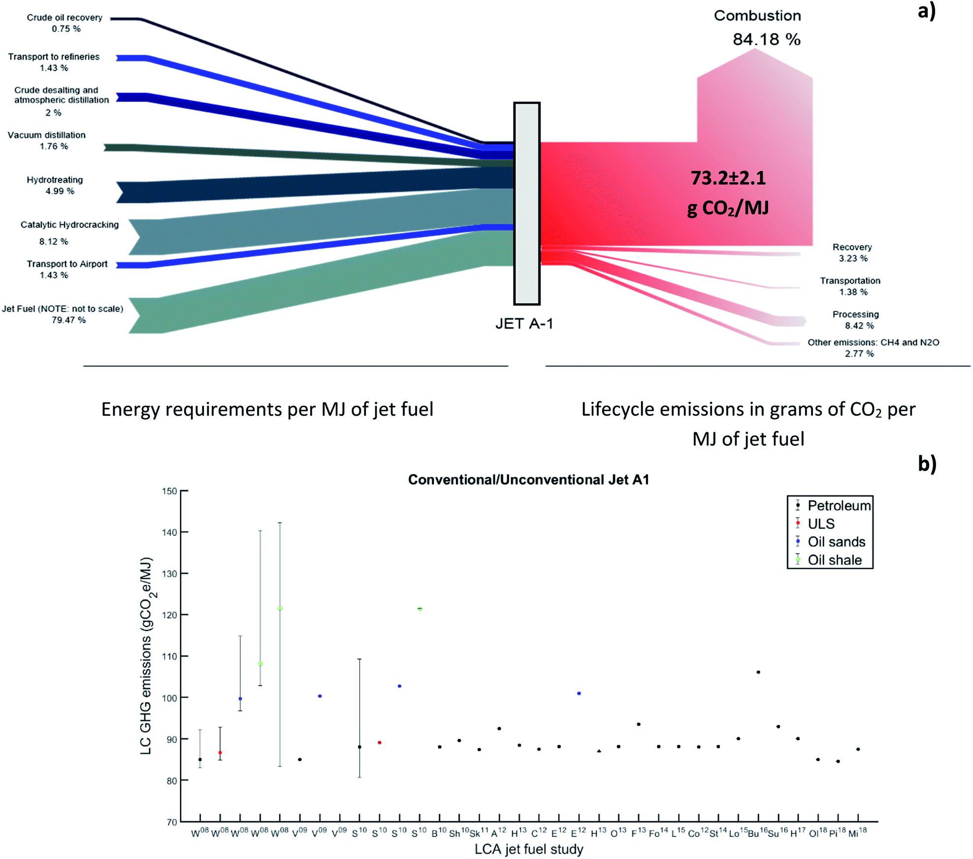Fig. 8 (a) Energy and lifecycle GHG emissions of conventional jet fuel; (b) Comparison of conventional/unconventional jet A1 emission factors. Horizontal axis illustrates the author and year of publication in superscript: W = Wong; V = Vera Morales and Shafer; S = Stratton; B = Bailis and Baka; Sh = Shonnard et al.; Sk = Skone et al.; A = Agusdinata et al.; H = Han et al.; C = Carter; E = Elgowainy et al.; O = Ou; F = Fan et al.; Fo = Fortier et al.; L = Li and Mupondwa; Co = Cox et al.; St = Staples et al.; Lo = Lokesh et al.; Bu = Budsberg et al.; Su = Suresh; Ol = Olcay et al.; Pi = Pierobon et al.; M = Michaelos et al.

The most energy intensive process is catalytic hydrocracking (8.12%) followed by hydrotreating (4.99%), while the largest contributor of GHG emissions is the fuel combustion in addition to processing (84.18%) which due to significant variation only the total contribution of CO₂ is presented (73.2 ± 2.1 g CO₂ per MJ). Taken as a whole, conventional jet fuel features a WtWa of approximately 95.3 ± 10.75 g CO₂e per MJ (ref. 47 and 77) based upon the literature available. Fig. 8(b) illustrates the distribution of these GHG results with error bars representing deviations from the sensitivity and uncertainty analyses where available. Of the more interesting works, Stratton compared the GHG emissions related to the origin of the oil field. The crude oil origin was averaged for the baseline scenario attributed to the countries that were researched in the study as well as the processing technique. The U.S. was selected for the crude oil origin low emission scenario and Nigeria was selected for the high emission scenario. The specifications indicated a refining efficiency of 93.5% for the baseline, 98% (low) using a straight run processing technique and 88% (high) using an HRJ/HEFA pathway. Results indicated 87.5 and 89.1 g CO₂e per MJ for jet A-1 and ULS, respectively.

The main contributor of GHG emissions is kerosene combustion. Interestingly, Stratton also performed an assessment of the non-CO₂ combustion emissions (see Section 4.4 for further discussion) through upscaling the CO₂ value raising the overall impact of GHG emissions by 2.47 times up to 180.8 g CO₂e per MJ accounting for all climatic impacts.

4.1.2 Unconventional crude oil (UCO). As discussed in Section 3.3.2, unconventional crude oil offers an alternative to conventional crude. Based upon the results of the literature in Fig. 8(b), UCO overall is considerably worse in terms of GHG emissions compared with crude oil over the entire lifecycle with a total study deviation of between 96.8 and 142.2 g CO₂e per MJ. The two types of unconventional crude – oil sands and oil shale is carried out by the literature. Wong for example conducted two assessments for Canadian oil sands. The first study was based upon surface mining with emissions reported to be around 99.7 g CO₂e per MJ. The second assessment was based upon in situ production and resulted in 108.2 g CO₂e per MJ. Stratton²⁰⁷ improved upon Wong's study by performing an environmental analysis of oils sands and oil shales, reporting total emissions of 102.7 and 121.5 g CO₂e per MJ. In addition, crude mixes were also assessed which looked into combining both crude types⁷⁸ which oil sands emitted 103 g CO₂e per MJ and the crude mix roughly equalled conventional crude, indicating no significant improvements was carried out to the emissions levels, although lower sulphur content was reported. From these results it appears that oil shale carries the highest level of GWP due to the mining and extraction processes, resulting in significantly worse GWP emissions than conventional crude oil.

4.1.3 Coal. In terms of the results of this feedstock, it is immediately clear according to Fig. 9, that coal is one of the worst performing pathways in terms of GHG emissions and in some studies up to six times worse without point source carbon capture. This can be confirmed across the literature in Wong⁴⁷ who conducted an analysis of coal with carbon capture (CC) and without carbon capture (WCC) technology, indicating that WCC produced emissions of 194.8 g CO₂e per MJ. Coal with CC produced much lower emissions of 91 g CO₂e per MJ. The sulphur content was recorded at 32 500 ppm and a further, more significant analysis evident in Vera-Morales and Schäfer¹⁵⁷ showed that liquid conversion efficiency was approximately 50% with WtP emissions that result in 115 g CO₂e per MJ using coal, i.e. 10× the level of conventional jet A1. Combustion emissions increase the GHG results to approximately 190 g CO₂e per MJ. This indicates that it contains twice the emission intensity of Jet-A1 derived jet fuel. If CC technology is applied, GHG emissions can be reduced substantially. GHG emissions indicate a total of 90 g CO₂e per MJ compared with 85 g CO₂e per MJ of petroleum-derived jet fuel. Stratton, a relation of Wong's earlier work conducted a similar study with results equalling 194.8 without CC and 97.2 g CO₂e per MJ with CC. In addition, Stratton also assessed a mixed blend of coal and switchgrass reporting a total GWP of 56.9 and 53 with and without CC. Elgowainy et al.⁷⁸ found that the total emissions were 225 g CO₂e per MJ for coal without CC installed and 105 g CO₂e per MJ with CC. Fig. 9 illustrates the results of the coal. Significant deviations can be seen indicating the impact of point source carbon capture across the studies.

Fig. 9 Comparison of LCA results of using coal for jet A1. Horizontal axis illustrates the author and year of publication in superscript: W = Wong; V = Vera-Morales et al.; S = Stratton; Sk = Skone and Allen; E = Elgowainy et al.

From the results of the coal LCA's, if point source carbon capture is installed within the gasification unit, there is potential to bring the total emissions to within the jet fuel production margins of crude oil. None of the investigations into the coal/gasification pathways for aviation fuel have included other characterisation factors apart from GWP but there is considerable evidence that the overall environmental impact of coal is considerably worse than that of crude oil.

4.1.4 Natural gas. According to Fig. 9, NG fairs better in the LCA results than coal when considering results with carbon capture and without. Wong⁴⁷ carried out two studies on NG (with and without CC).

His work originated in North America with the pathway data being available in the GREET LCA software (see Section 2.3.1). The analysis assumed a standalone FT plant which aimed to maximise the production of FTL and include tail gas recycling from F–T reactors. The study aimed to produce acceptable levels of energy to fuel its internal processes with no additional excess.

In addition, another pathway focusing on hydroprocessing of long chain liquid products estimated that 100.4 and 87.3 g CO₂e per MJ would be produced from NG, WCC and with CC technology, respectively. Two out of the four studies indicate much worse GHG emissions than the reported distribution of results of conventional jet A1. In another study by Vera-Morales and Shafer,¹⁵⁷ for example, results in terms of energy use within the fuel-cycle was the equivalent of 0.68 MJ per MJ of jet fuel (they assumed a gas-to-liquids conversion efficiency of 60 percent). GHG emissions were approximately 25 g CO₂-eq per MJ². When combustion is included, GHG emissions equalled 99 g CO₂-eq per MJ, a 16% increase over conventional jet fuel.

When using CC, reductions in CO₂ emissions (5.8 g CO₂-eq per MJ) becomes considerably lower than conventional jet fuel. Some studies such as Elgowainy et al.⁷⁸ from the Argonne National Laboratory estimated a 63% process efficiency for producing FT diesel which is comparable to the other studies. Their results indicated that up to 1 750 000 (J/MJ) of WtWa fossil energy were utilised by NG and a marginal amount of petroleum energy (J MJ⁻¹). Emissions resulted in 115.34 g CO₂e per MJ. In terms of trends, most of the results for NG tend to stay within the jet A1 margins and with carbon capture can perform slightly better than crude oil production.

4.2 Coal and biomass

Studies combining both coal and biomass via gasification/FTL have been reported comprising assessments of both coal and either corn stover or switchgrass (see Tables 2 and 3). The main impacts of corn stover indicates the extraction phase carrying the biggest burden due to the use of fossil fuels. This includes windrowing, baling and the transportation of the corn stover plant to a suitable location in the field. Fertiliser also possesses a significant impact.¹¹⁸ The impact of cultivation is not applied to corn stover (corn is its by-product). Across the literature, transportation fluctuates widely due to differences in biomass yields and bio refinery capacity. Estimated figures in terms of capacities for pyrolysis bio refineries are between 2000–3000 dry tons of biomass per day.^118,208Fig. 10 illustrates the results of coal and biomass from the literature. Half of the baseline results are worse than the reported conventional jet A1. Manufacturing jet fuel through the combination of corn, coal or corn stover uses the established gasification/FTL process pathway. Crucially, the biomass feedstock fraction is a key parameter for LCA results.^208–211 Select studies include Skone et al.¹⁵⁹ where they carried out a large case study on the gasification/FT process pathway assessing 10 different scenarios of aviation fuel production from coal and various concentrations of switchgrass. The results are highly detailed giving a range of between 55.2 or 37% reduction (scenario 8 using displacement with best estimate value) to 98.2 g CO₂e per MJ or 12% increase (scenario 1 using displacement with best estimate value) compared to conventional jet fuel i.e. 88.1 g CO₂e per MJ. Elgowainy⁷⁸ highlighted that Coal mixed with biomass (forest residue) produces total emissions equalling approximately 140 g CO₂e per MJ.²¹² Others studies²¹³ focused on the assessment of coal and corn stover to produce FT liquids. The combination of liquids tended to include diesel, jet and naphtha. Corn stover is arguably the best candidate for the gasification/F–T pathway due to its minimal land use requirement.²¹⁴ The forming and extraction of corn stover, the mining of Bitumen coal and cleaning, and FT production were all emission intensive processes. The harvested corn stovers nutrient content was calculated through mass equations and assumptions were made on N₂O emissions in that they can be represented as the same as synthetic nitrogen and nitrogen in crop residues i.e. supplemental nitrogen fertiliser (nitrification and denitrification) were assumed to be zero.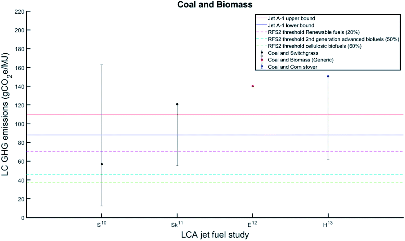

Fig. 10 Comparison of LCA results of using coal combined with a variable biomass fraction for jet A1. The process pathway adopted was the gasification/FTL process pathway. Horizontal axis illustrates the author and year of publication in superscript: S = Stratton; Sk = Skone and Allen; E = Elgowainy et al.; H = Han et al.

In terms of transport of coal and biomass, the literature assumed various distances, based upon the above studies from both pyrolysis and gasification/FTJ pathways. The source of GHG emissions for coal mining included abandoned mines, degasification, post-mining operations and non-combustion CH₄ emissions.²¹⁵ The study in particular identified both surface mining and underground activities, where non-combustion emissions of CH₄ differ radically. Coal mining and cleaning also includes the energy costs of mining above and below ground. Biomass shares of around 20% are considered to be the baseline variable for the study. As expected, the increase in corn stover usage reduces the GHG impact of aviation fuel production. The results of CC with improved efficiencies indicated 98 g CO₂e per MJ while reduced efficiencies indicated 152 g CO₂e per MJ.

4.3 Biomass

4.3.1 First generation biomass. The production of aviation fuel from first generation biomass is taken primarily from the HEFA/HRJ pathway and is in direct conflict with human food supply, invoking significant land use requirements.

The U.S. for example historically invested in soybean oil in order to produce biofuel indicating 30.9 g of N, 210 of potassium oxide (K₂O), 113.4 g of phosphorous pentoxide (P₂O₅), where data was taken from the National Agricultural Statistics Service.²¹⁶ Around 1.32% of the N from indirect and direct conversion in fertilisers and soybean biomass in the field leads to emissions of N₂O.⁶⁴ Oil extraction energy requirements is approximately “3590 Btu lb⁻¹ of oil; 5.4 lb of soybeans yield 1 lb of oil and 4.4 lb of soy meal”.²¹⁷ Livestock feed based on soybeans is displaced via soy meal. For the displacement ratio, approximately 1.2 lb soybeans represented 1 lb of soymeal.

Fig. 11(a) illustrates a comparison of all of the 1^st generation biomass LCA studies. The results of allocating first generation biomass to be used for AAF production comprises 11 studies (30%)^{47,78,91,105,119,169,179,196,198,201,204} which all performed a WtWa of aviation fuel produced by first generation biomass. There were a total of five feedstocks that were reported from the HEFA process pathway consisting of sugarcane (six studies), soybean (four studies), corn grain (three studies), rapeseed (two studies), and canola (one study). These feedstocks were one of the first to be assessed for aviation fuel production and consist of additional co-products where available which in turn may affect the distributions of results of the LCA.

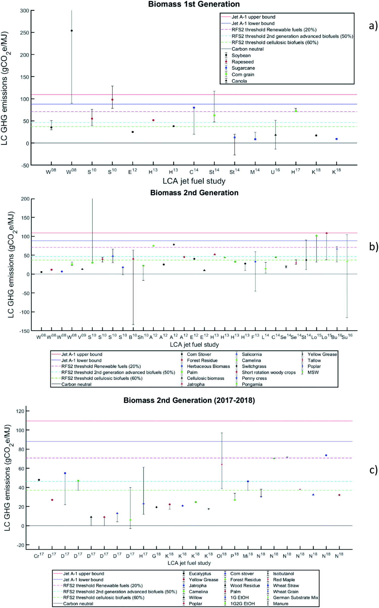Fig. 11 LCA results of first (a), second (b) and second (2016–2018) (c) generation biomass with error bars representing all scenarios in the specific study. Upper and lower bounds of conventional jet A1 derive from the distribution of ULS and crude oil results in Fig. 8. Dotted lines represent the 2^nd edition of the renewable fuel standard, illustrating the required reduction percentile for the fuel to be certified with RFS2. Horizontal axis illustrates the author and year of publication in superscript: A = Agustinata et al.; B = Bailis and Baka; Bu = Budsberg et al.; C = Cox et al.; G = Ganguly et al.; E = Elgowainy et al.; H = Han; K = Klein et al.; L = Li and Mupondwa; Lo = Lokesh et al.; Mi = Michailos et al.; M = Moreira; N = Neuling and Kaltschmitt et al. Ol = Olcay et al.; P = Pierobon et al.; U = Ukaew et al.; S = Stratton; Se = Seber et al.; Sh = Shonnard et al.; St = Staples et al.; Su = Suresh et al.; U = Ukaew et al.; W = Wong.

As can be seen in Table 4, all four allocation methods were involved across the studies. Overall results by the displacement allocation method indicated between −27–639 g CO₂e per MJ. Staples et al.²⁰¹ in their comprehensive analysis of sugarcane recorded the best results out of the 1^st generation biomass feedstocks from the advanced fermentation pathway with optimal feedstock-to-fuel efficiencies and utility requirements with overall variability of their results being high. Wong⁴⁷ on the other hand calculated that depending on land use requirements, the results of soybean could lead to 639 g CO₂e per MJ depending on the feedstock that is being displaced or in this instance replacing soybean with its soy meal co-product.

Overall results for the energy allocation method led to between 26–600.3 g CO₂e per MJ. De Jong⁸³ recorded the lowest GHG emissions for sugarcane from the ATJ pathway with the most energy intensive process coming from the conversion of the feedstock, performing better than the STJ pathway. The highest emissions stem from the worst land use scenario for soybean in Wongs study. Different land use change scenarios were applied to the cases from Wong which were also applied to three or four unique pathways.

In terms of mass allocation, the overall distribution of results equated to between 21–131.5 g CO₂e per MJ for AAF production from soybean. Both of these results come from Wongs mass allocation scenario where the lowest number represents the exclusion of land use and the highest number representing the results are inclusive of land use. These results are dependent on the mass of the co-products. For example, two key co-products tended to be produced from the soybean plant, which consists of soy oil and soy meal (which is a livestock feed⁷⁸). In terms of mass, soy meal for example has a higher mass allocation (about 5 times that of the extracted soy oil.) although its energy to mass ratio is lower.

Finally, market allocation resulted in deviations of between 6.8–289.0 g CO₂e per MJ. The lowest emissions were based upon the sugarcane feedstock being produced through advanced fermentation that was carried out by Staples et al. Once again, due to land use change accounting for over 87% (253.8 g CO₂e per MJ) of the result the most emission intensive pathway was Wongs evaluation of the Soybean feedstock.

Overall, when land use is included into the LCA calculation, soybean being produced through HEFA/HRJ is the most emission intensive feedstock out of the 1^st generation biomass pathways. In addition, Stratton later updated the datasets of soy oil that Wong originally assessed in order to determine emissions that were more related to HRJ/HEFA based process pathways. Land use changes and their impacts were also updated and refined as they possessed substantial damage effect on the LCA AAF fuel including long-term impacts.

4.3.2 Second generation biomass. As discussed earlier (Section 3.3.4), 2^nd generation biofuels originate from biomass that cannot be consumed by humans, including plants, animal waste such as tallow and Municipal Solid Waste (MSW) which can be used specifically to produce aviation fuel. Fig. 11(b) and (c) illustrates the results of the second-generation pathways. The results of allocating second generation biomass in order to produce aviation fuel consists of 28 studies (75% of the literature)^{47,77,78,81,82,105,116,119,157,159–162,171,172,174,178,182,196,199–205,218} which all performed WtWa analysis of aviation fuel produced by second generation biomass. There were a total of 18 feedstocks that were reported across five different pathways. These pathways consisted of: HEFA/HRJ (15 studies), gasification/FT (12 studies), advanced fermentation/STJ (six studies) and alcohol-to-jet (five studies). The majority of the feedstocks consist of lignocellulosic biomass that is in an abundant supply globally, hence this type of feedstock is a popular choice for the production of aviation fuel.

Referring to Table 4, all four allocation methods were once again utilised throughout the various studies and the results are represented through these methods. Overall results by the displacement allocation methods indicated between −134 and 98 g CO₂e per MJ. The best displacement performance stems from Bailis and Baka¹⁷⁴ who compared the LCA emissions of synthetic paraffinic kerosene (SPK) derived from the Jatropha curcas feedstock produced in Brazil. The findings from this study considered four tonne dry fruit per ha through drip irrigation using current logistical planning through energy-allocation. A 20 year lifetime for plantation with zero LUC was assumed resulting in 40 g CO₂e per MJ of produced fuel, performing better than jet A1 by 55%. When including LUC carbon stocks the results vary from 50 tonne C per ha (if it is grown within woodland) increasing to 10–15 tonne C per ha (grown within former agro-pastoral regions). GHG emissions can fluctuate from 13 c if the Jatropha plant is grown within previously established agro-pastoral lands (85% decrease) to approximately 141 g CO₂e per MJ, if Jatropha was grown via cerrado woodlands (60% increase). However, the best performance stems from using the seedcake and husk as boiler fuel and selling the remaining excess electricity back to Brazil's national grid. The high end emissions from displacement are from Staples who estimated that switchgrass may feature emissions of 89.8 g CO₂e per MJ. Once again, the variability in the technology of advanced fermentation performance which affects the feedstock-to-fuel conversion efficiency in addition to the utility requirements contribute to this result.

In terms of energy allocation the best results were obtained from Suresh et al. who calculated −115.5 g CO₂e per MJ from ATJ process pathways which were sensitive to associated fuel yields co-product allocation method, feedstock transportation distance, MSW composition, plant scale and waste management strategy displaced. However, the most prominent factors for such a result is the non-biogenic fractions where were assumed to be 0% for −115.5 and 65% for a results of 104.2 indicating that the results are highly sensitive to MSW's organic fraction. The worst results were carried out by Strattons⁷⁷ work who performed a comparative analysis of switchgrass, Jatropha and Salicornia with biomass credits of −222.7, −70.5 and −105.3 g CO₂e per MJ due to photosynthesis. For switchgrass, offsetting total LCA emissions if land use changes are applied (−19.8), negative WtWa emissions of −2 g CO₂e per MJ are obtained, providing a minor carbon sink and 17.7 g CO₂e per MJ taking into account unavoided land use. However, the worst land use scenario indicated 698 g CO₂e per MJ.

In terms of mass allocation, the range of results indicated between 10–47.1 g CO₂e per MJ. Elgowainy et al.⁷⁸ calculated GHG regulated emissions for cellulosic biomass. The results were incorporated into the expanded transportation (GREET) model. The results of the corn stover from pyrolysis indicate approximately 39.6 g CO₂e per MJ (55% reduction) while cellulosic biomass gave WtWa results of around 10 g CO₂e per MJ or 85% reduction which is the best result in the literature. Crossin¹⁷¹ estimated the worst performing feedstock from mass allocation from the Mallee Eucalyptus feedstock using a theoretical biorefinery operating in the great southern region of Western Australia. GHG emissions were reduced by up to 40% compared to crude oil and further reductions can be applied such as capturing methane emissions for the production of hydrogen and the use of co-produced bio-diesel. The potential impact of environmental benefits were sensitive to potential food displacement and co-production.

Finally, for market allocation, the worst result that was recorded was from Wong where palm oil that was inclusive of land use indicated total emissions of 139.0 g CO₂e per MJ. This was calculated through assigning 97.9% of the total feedstock cost to the palm oil ($0.78 per kg) and palm kernel oil ($0.78 per kg) and 2.1% to the palm kernel expeller. The market value of palm oil in 2008 ($0.15 per kg). The best result was recorded in Capaz et al.¹⁸² with sugarcane bagasse and straw indicating total emissions of 8.2 g CO₂e per MJ.

4.3.3 Third generation biomass. Fig. 12 illustrates the GHG results of third generation biomass showing high variations in terms of GHG's and significant uncertainty. As discussed earlier in Section 3.4.5, 3^rd generation biofuels consist entirely of algae/microalgae feedstocks. They do not conflict with food for human consumption, land use is minimal and their energy content is superior than lignocellulosic biomass (2^nd generation). For example, Vera-Morales and Schäfer's²¹⁹ study on microalgae offered early promising insights from the perspective of productivity as lower land requirements and food resource avoidance offer considerable benefits. Algae productivity consisted of 30 g per m² per day and lipid contents of 50%.²²⁰ Energy requirements (0.44 MJ MJ⁻¹) stems from CO₂ from coal power plants that fertilises algae resulting in approximately 32 g CO₂e per MJ (40% reduction). Captured CO₂ emissions from coal power plants result in 86 g CO₂e per MJ fuel within the threshold of conventional jet fuel results in Fig. 8. If clean flue gas is used 19 g CO₂e per MJ is produced. The results of allocating 3^rd generation biomass to the production of jet fuel consists of 12 studies representing 32.4% of the literature.^{77,78,80,125–127,157,162,166,196,202,221} Two different pathways have been used to produce algae/microalgae: HEFA/HRJ (nine studies representing 24.3%) and HTL (two studies or 5.4%).

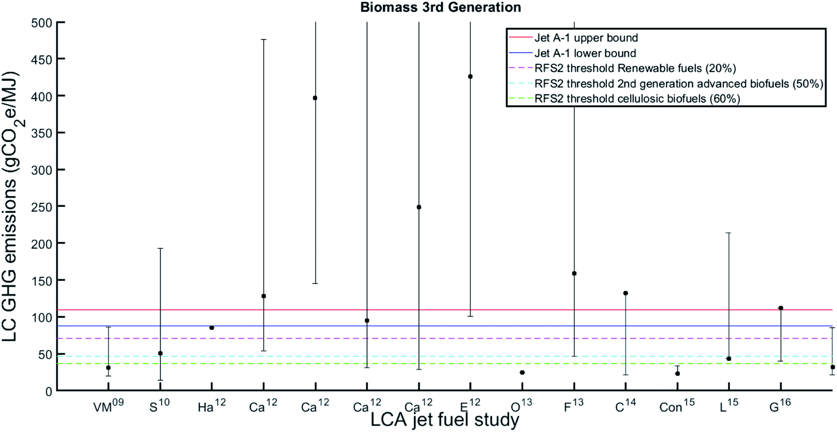Fig. 12 LCA results of third generation biomass with error bars representing all scenarios in the specific study. Upper and lower bounds of conventional jet A1 derive from the distribution of ULS and crude oil results in Fig. 8. Dotted lines represent the 2^nd edition of the renewable fuel standard, illustrating the required reduction percentile for the fuel to be certified with RFS2. Horizontal axis illustrates the author and year of publication in superscript: V = Vera-Morales et al.; S = Stratton; H = Han et al.; Ca = Carter; E = Elgowainy et al.; O = Ou et al.; F = Fortier et al.; CO = Connelly et al.; Lokesh et al.; Guo et al.

With reference to Table 4, all four allocation methods were used to assess the environmental performance of 3^rd generation feedstocks and the results are once again compared using the different methods in order to identify trends and the most dominant pathway processes. From the perspective of displacement, GHG emissions from Microalgae were between 14.1–1020 g CO₂e per MJ, representing a significant variation in results across the displacement method alone. For the best result, Stratton⁷⁷ conducted an LCA of algae-derived jet fuel from the HEFA/HRJ pathway. From an analysis of the study using displacement for the low and baseline scenarios, the most notable differences between the cases that have been conducted lie within the recovery phases, as well as WTT CH₄. CO₂ emissions are appended from injection, dewatering and drying of the algae. Uncertainties surrounding N₂O emissions (algae ponds and flooded rice fields have been given similar cultivation penalties). Little information exists on N₂O formation from algae ponds. N₂O only contributes 16% of WtWa GHG emissions. The worst emissions stem from Carter⁸⁰ who carried out an environmental LCA on microalgae production (U.S.) using horizontal serpentine tubular packed bed reactors.

GHG emissions, energy, land use and water consumption are sourced in the “direct cultivation, harvesting, dewatering, and drying”.⁸⁰ In terms of cultivation technologies, GHG emissions and production costs were really sensitive within the context of lipid content, inputs and microalgae productivity although harvesting technologies were more sensitive for the open raceway ponds.

In terms of the energy allocation method overall results indicated between 17.23–851.9 g CO₂e per MJ. The best result consists of a detailed study by Guo et al.¹⁶⁶ who performed an LCA of microalgae based aviation fuel. Lipid content on fossil fuels and GHG emissions are relatively close and energy consumption is 0.68 MJ MJ⁻¹ and GHG emissions of their entire study were between 17.23–51.04 g CO₂e per MJ. Effectively, this is an increase of between 59.70–192.22% with higher lipid content. Total energy requirements is reduced (2.13–3.08 MJ MJ⁻¹ or 0–47.10%) with lower N efficiency of between 75–50% in terms of recovery. The worst results of the literature stem from Ou et al.¹⁶⁵ who studied open ponds using datasets that correlate to the Tsinghua University LCA Model (TLCAM) which was explored in Section 2.2.3. Most of the attention was based upon the energy recovery via biogas production and also combined heat and power from leftover biomass after lipid extraction. This includes CH₄ emissions of biogas production and N₂O emissions of digestates which can be used as agricultural fertiliser. These emissions stem from the assumptions of low algae productivity, and high energy use in CO₂ acquisition for cultivation with 140 kW h per tonne, algae harvest and lipid extraction.

For mass allocation overall results were between 20 and 131.9 g CO₂e per MJ with Vera-Morales et al. offering the best result assuming that flue gas was utilised as an input for CO₂ extraction and point source carbon capture was implemented on site. The worst result on the other hand was discovered by Fortier et al.¹²⁵ who conducted a study of microalgae via HTL (1 GJ functional unit) which was “cultivated in wastewater effluent”. Two distinct scenarios were carried out in a refinery and a wastewater treatment plant. Upon assessing the results, refinery transportation and waste nutrients dominated the LCA. Levels of heat integration introduced a great deal of sensitivity to the LCA in addition to the heat source and the solids content of the dewatered algae. In their most optimised study up to 76% reduction compared with jet A1 can be attained with minor improvements to the aforementioned sensitivity parameters.

Finally, the market allocation gave a distribution of between 31–2020 g CO₂e per MJ. This distribution was carried out entirely within Carters study, who assessed the difference between open raceway ponds using wet lipid extraction against horizontal serpentine tubular reactors which were significantly more energy intensive resulting in significantly high levels of GHG emissions.

4.4 Other environmental factors from combustion

4.4.1 Estimating combustion effects during flight. The estimation of GHG emissions during the combustion phase is open to controversy as there is a lack of agreement on how to suitably model the impact of the aircrafts wake. Thus, non-CO₂ effects during flight has received a significant amount of attention recently and these studies can be read here.^222–225 Key issues to resolve are the methodologies that are being used to calculate emissions during each phase of a commercial aircraft i.e. taxiing, taking off, cruising and landing. ICAO has reported that due to a lack of agreement on the methodologies quantifying GHG estimations other than CO₂, there are no official results available.

4.4.2 Water vapour and water contaminated fuel. Water vapour when produced at high altitude contributes significantly to global warming.²²⁶ Although the residency period does not get mentioned in the literature much it has been estimated as 8.9 ± 0.4 days,²²⁷ however, it is currently difficult to quantify such emissions using the GWP20 and GWP100 characterisation factors. Water contaminated fuel when combusted produces additional water vapour in its wake and it is thought that the aromatic component plays a role in the solubility of water in jet fuel.^225,227

4.4.3 Additional environmental results. For kerosene based fuel, other studies explored additional characterisation factors. For example, Koroneos et al.²²⁸ used a functional unit of 1 kg of kerosene production. Ozone depletion indicated 1.84 × 10⁻⁸ while acidification had the highest impact at 7.75 × 10⁻⁴ where 96.04% is due to combustion. Eutrophication (1.93 × 10⁻⁴ air and 1.06 × 10⁻⁵ water) and summer smog (2.76 × 10⁻⁴) were less severe.

A select number of studies carried out an environmental analysis of the AAF product using the following characterisation factors: smog, eutrophication, eco-toxicity, acidification, carcinogenics, non-carcinogenics, respiratory effects, water use and land use. Table 5 highlights the results of these assessments.

Table 5 Further environmental factors in the alternative jet fuel literature

Feedstock	Smog (g O3e per MJ)	Eutrophication (g PO4e per MJ)	Eco-toxicity (day per CTU per MJ)	Acidification (g SO2e per MJ)	Carcinogenics (CTUh MJ^−1)	Non carcinogenics (CTUh MJ^−1)	Respiratory effects (g PM2.5e MJ^−1)	Water use (L)	Land use (m^2 a)
Koroneos et al.
Kerosene	2.76 × 10^−4	2.04 × 10^−4		7.75 × 10^−4
Cox et al. – displacement allocation
Sugarcane	—	44	5.11 × 10^−7		—	—	—	14.7	38.9
Pongamia	—	12	1.10 × 10^−9	—	—	—	—	1.18	7.8
Microalgae	—	11	8.60 × 10^−10	—	—	—	—	1.39	7.0
Cox et al. – energy allocation
Kerosene	—	7	1.40 × 10^−10	—	—	—	—	0.001	0.003
Sugarcane	—	15	5.20 × 10^−10	—	—	—	—	1.56	5.1
Pongamia	—	9	5.20 × 10^−10	—	—	—	—	0.55	4.5
Microalgae	—	9	4.20 × 10^−10	—	—	—	—	0.64	6.8
Ganguly et al. – energy allocation
Forest res.	9.17	1.12	283.03 CTU	0.39	−1.04–10^7	9.55–10^6	−0.34	—	—
Pierobon et al. – mass allocation
Forest res.	9.54	0.03	47.46 CTU	0.47	5.40 × 10^−8	7.55 × 10^−6	−0.07	—	—
Pierobon et al. – displacement allocation
Forest res.	11.03	−0.09	162.97 CTU	0.88	1.94 × 10^−8	2.51 × 10^−5	−0.28	—	—

---

Cox et al. carried out an analysis of the effects of eutrophication using displacement allocation (44, 12, and 11 g PO₄e per MJ for sugarcane, pongamia and microalgae respectively) indicating that sources of nitrogen oxide (NO_x) exhaust gases from combustion in jet engines from the combustion of bagasse in addition to biogas and light gases from fossil fuels were the most dominant. According to Cox et al., sugarcane also has the potential for field emissions of the nutrients (N and P) which originate from the sugarcane growth which can amount to higher levels of eutrophication as opposed to pongamia and microalgae cases.

Eco-toxicity potential trends stem from the release of heavy metals and organics which originate from chemical production and electricity generation. Grid displacement in terms of electricity provides the lowest toxicity score. Further comparisons of different impact assessment methods are required as the configuration of weights differ between the characterisation factors i.e. greater priority for environmental burden is given to pesticides as opposed to metals and organics.

The key process responsible for water use was irrigation for the growth of pongamia and sugarcane. The supply of water to the ponds that hold algae are carried out in order to compensate for key evaporative losses.

Pongamia (1.18 L or displacement and 0.55 for energy allocation) features the lowest water use and sugarcane possesses much higher use in more arid climates such as Australia, indicating that the environment is a marker to determine water use in feedstock production for AAF.

In terms of land use, the pongamia cause offers the best result due to high cultivation efficiency (4.5 m²/100 MJ), followed by sugarcane (5.1/100 MJ) and microalgae (6.8/100 MJ). All three pathways can be considered relatively low compared to biodiesel.

Studies by Ganguly et al.¹⁷² and Pierobon et al.²⁰⁵ using energy, mass, and displacement allocation on forest residue were carried out with some deviations in their results. Eutrophication (1.12, 0.03 and −0.09 g PO₄e per MJ) and eco-toxicity (283.03, 47.46 and 162.97 CTU) can be mostly attributed to the wastewater treatment process, releasing acetic acid, furfural, nitrates, lignosulfonic acid, nitrogen dioxide, phosphates, soluble sugars and sulphur dioxide. The key contributor to the smog characterisation factor (9.17, 9.54 and 11.03 g O₃e per MJ) stems from combustion during flight (representing just under half of the total impact). This factor is also related to acidification 0.39, 0.47 and 0.88 g SO₂e per MJ (33.7%). Additional impacts arising from combustion include carcinogenics impact (−1.04–10⁷, 5.40 × 10⁻⁸ and 1.94 × 10⁻⁸ CTU_h MJ⁻¹) and non-carcinogenic impact (9.55–10⁶, 7.55 × 10⁻⁶ and 2.51 × 10⁻⁵).

5. Prospective and conclusion

5.1 Alternative ‘drop in’ aviation fuels for current technologies

The following section explores possible alternative feedstocks and pathways which could be used to produce jet fuel, however, they do not yet possess LCA results from the literature specifically referring to the jet fuel fraction. Nevertheless, such alternatives may become important in the future in a bid to avoid land use and conflict with food.

5.1.1 Oleaginous yeasts. An opportunity exists to produce jet fuel from oleaginous yeasts which are lipid based microorganisms.^229–236 Their ability to produce such lipids is relatively high (20% of their dry weight can produce such organic compounds) and it may also be possible to increase lipid content to 70% under certain conditions offering excellent potential as a jet fuel provider. Unfortunately, the lipid extraction process phase has to currently be performed using solvents that include a wide variety of toxic chemicals such as petroleum hexane as well as a mixture of hydrocarbons. Such extraction methods will have to be replaced in the future for LCA performance to remain competitive with the core feedstock contributions to biomass in Section 4. A non-LCA based study on oleaginous yeasts towards the production of jet fuel currently exists. Breil et al. performed an experimental study on jet fuel production with two theoretical sub-units based on the extraction of oil from the Yarrowia lipolytica organism. They hypothesize that ethyl acetate, CPME and MeTHF could replace hexane solvents in order to support the energy required to evaporate 1 kg of solvent,²²⁹ however, it remain to be seen when exactly such innovations will take place.

5.1.2 Waste carbon, water and materials. There is promising potential to produce jet fuel from waste carbon such as CO₂ and water due to the presence of H₂. Current technologies that are available which can help make this happen is the use of solid oxide co-electrolysis (SOEC)^237–241 which separates O₂ from H₂O through reverse water–gas shift and microbial fuel cells (MFC's). Microbial fuel cells (MFC's) which are a rapidly evolving field and consists of new forms of energy generation in which no universally defined terminology has been given.^242–249 MFCs offer a promising technology to produce liquid fuels from wastewater leading to the potential production of aviation fuel and although this particular field is still in its infancy, there has been significant progress, as summarised here.^36,250–253 In the past decade, it was discovered that the alkane biosynthesis pathway could be created from cyanobacteria in the range of C13–C17 alkanes and alkenes.²⁵⁴

Waste carbon from residues and other materials are in abundant supply. Throughout the studies, there is a potential opportunity for a future process pathway that can take CO₂ from industrial sources such as a coal power plant, oil refinery or steel industries in order to produce H₂ rich syngas.²⁵⁵. This technology allows CO₂ to be reduced into its constituent elements and together with biomass from gasification performs co-valorisation, producing two syngas streams with one rich in CO and the other in H₂. Recent technological advances indicate that SOEC's may be affordable while providing high performance and low temperature SOEC due to recent advances in Ni thin-film electrodes on porous alumina templates.²⁵⁶ Solid oxide co-electrolysis²⁵⁷ would effectively allow for a rich H₂ syngas to be produced while the biomass would enter a gasifier and produce a rich CO syngas, eventually combining them through FT to produce carbon neutral aviation fuel. CO₂ pipelines would transport the CO₂ from the industrial source to the bio refinery²⁵⁸ and directly into the SOEC unit.

5.2 Alternative aviation fuels for modified aircraft and future technologies

This section discusses potential future aviation fuel sources that require non-conventional modification of an existing aircrafts system.

5.2.1 Ethanol and methanol. Ethanol, while currently being used in land vehicles in small quantities (known as E10 with a 1 : 10 fuel ratio in U.S.), there are issues which go against its use. The first is that ethanol like 1^st generation biomass possesses conflicts with human consumption and secondly, it is very difficult to store the chemical safely²⁵⁹ due in part to its low flash point. Issues also arise during flight where a combination of difficulties may include fuel system vapour lock, which is where liquids will change their state to a gas within the fuel delivery system. There are several methods to reduce vapour lock and improve the safety of the use of ethanol, but it requires substantial investment in the modification of current infrastructure and aircraft. Also, there is a lower level of performance overall in terms of energy efficiency (40% reduction compared with conventional jet fuel).²⁶⁰

Methanol is a by-product of the fossil fuel production process of coal and NG (described in Sections 3.2.3 and 3.2.4). However, it can also be produced from biomass from both woody and MSW's and can also be produced from CO₂via carbon capture technologies. Methanol production is one of the key drivers for the persistence of NG production, it is 70% energy efficiency and almost the entire product is methanol (99%).²⁵⁹

5.2.2 Hydrogen. Hydrogen sourced feedstock's can become a suitable future aviation fuel^{259,261–265} and can be extracted from a wide variety of sources. Hydrogen productions paths may include direct water splitting from renewable energy, as a by-product of electricity production from electrolysis from radioactive waste and also from the cracking and steam reformation process from fossil fuels once carbon sequestration has taken place.²⁶¹ Hydrogen has a calorific value that is 2.8 times higher than kerosene, however the volume of hydrogen is four times more so this higher energy content will be offset somewhat in addition to a heavier tank. In order to be utilised. H₂ needs to be stored in liquid form (LH₂) in cylindrical storage tanks with appropriate insulation and pressure differentials indicating that the tanks will require non-conventional modifications. Ammonia can be converted into hydrogen pathway (below).

5.2.3 Ammonia. Ammonia is considered to be one of the most highly produced inorganic chemicals²⁶⁶ and offers an abundant supply of feedstocks as a potential replacement to fossil fuels, therefore it can be used as a cleaner source of fuel production. It currently cannot be used in conventional engine technologies due to its extremely narrow flammability spectrum although it has a remarkably high octane rating of 120. Ammonia can be fed into a fuel cell that can produce energy with the calorific value of ammonia being much lower than kerosene at 22.5 MJ kg⁻¹. If the water vapour is not condensed the calorific value will be 21% less than the aforementioned number. Carbon monoxide, hydrocarbons and soot cannot be produced as ammonia does not feature any carbon therefore it burns very cleanly with minimal contaminants. Also it is possible to convert ammonia to a hydrogen pathway using the sodium amide process and can also be converted as fuel to a proton exchange membrane cell. Ammonia solid oxide fuel cells (SOFC's) can also be used for on board power production. It is possible to use liquefied ammonia with or without the use of fuel cells. When assessing the scenario without the fuel cell a liquefied ammonia tank, dissociation and separation unit for decomposition of ammonia and an internal combustion engine rounds off the pathway which powers the vehicle. In the second configuration the fuel cell drives the power and it is supplemented with the internal combustion engine.

There are two key disadvantages for using ammonia in aircraft. The first is that it possesses a low energy density compared with hydrocarbon-based fuels and although it burns cleaner, it is still toxic via the production of other caustic substances, which will be distributed at high altitude. This has slowed down its integration with the global transportation system.

5.2.4 Liquid natural gas (LNG). Liquefied natural gas may offer supplemental power to existing aircraft through modification of the fuel delivery system.²⁶⁷ As NG is much cheaper than traditional kerosene based jet fuel this is an attractive option once the retrofitting has been carried out. Withers et al. in their study on comparing LNG (50% kerosene based fuel in terms of energy content included) with the NG Fischer–Tropsch pathway (with 50% of kerosene based jet fuel by volume) indicated that a 39%, 24%, 1% and 47% reduction in CO₂ NO_x, black carbon and hydrocarbons respectively is possible.

5.3 Conclusion

A wide variety of AAF LCA studies have been published within the last decade using vastly different approaches to the adoption of process pathways. In addition, the actual methods that were used when carrying out the LCA are also utilised differently, meaning it is very difficult to draw comparisons with other studies. In particular, the four allocation methods applied to aviation fuels, namely mass, energy, market and displacement, cause large fluctuations in the results of the LCA's. However, the basic benchmarking of the different approaches has shown that when producing AAFs from biomass, there is great promise being shown in the literature. Compared with the other process pathways under review, HRJ and FTJ fuels appear to show the biggest potential in terms of the greatest reduction of GHG emissions as they have a high FRL level and are already certified to be produced commercially with a 50% blending ratio compared with conventional jet A1.

Many studies highlighted the key drawbacks in relation to biodiesel and bio-alcohols as aviation fuels due to poor fuel composition properties as highlighted in Tables 2 and 3. Using liquid hydrogen and methane are favoured, however high production cost and less suitability to the confines of the turbofan conventional engine seriously limits their capabilities and potential impact. A variety of serious challenges exist, mainly land use and agricultural emissions and levels of distribution. There is however increased backing of international governments with a variety of organisation providing certification and recommendations, pushing policy forward to enable the delivery of sustainable fuels more quickly. It is here that scaling up can be supported along with necessary commercialisation in addition to supply chain infrastructure. Finally, other characterisation factors need to be applied in order to fully embrace LCA as an environmental accounting method. As only 10% of the literature refer to the GWP only, it is imperative that these methods be used more fully. This should be the primary goal of future investigate work in order to fully decarbonise the aviation sector.

Conflicts of interest

There are no conflicts to declare.

Acknowledgements

The authors wish to acknowledge UK funding of the project “Low carbon jet fuel through integration of novel technologies for co-valorisation of CO₂ and biomass” by the Engineering and Physical Sciences Research Council (EP/N009924/1). We would also like to thank researchers Kourosh Kian for his expertise in combustion and petroleum engineering, Caleb Woodall and Helene Pilorge for providing additional support in critically reviewing and improving the manuscript.

References

1. IPCC, Global Warming of 1.5 °C, Intergovernmental Panel on Climate Change, Geneva, Switzerland, 2018.
2. F. Cherubini, N. D. Bird, A. Cowie, G. Jungmeier, B. Schlamadinger and S. Woess-Gallasch, Resour., Conserv. Recycl., 2009, 53, 434–447.
3. J. D. Scheelhaase and W. G. Grimme, J. Air Transport. Manag., 2007, 13, 253–263.
4. L. Luo, E. van der Voet, G. Huppes and H. A. U. De Haes, Int. J. Life Cycle Assess., 2009, 14, 529–539.
5. F. Cherubini, A. H. Strømman and S. Ulgiati, Resour., Conserv. Recycl., 2011, 55, 1070–1077.
6. M. Brander, R. Tipper, C. Hutchison and G. Davis, Technical Paper: Consequential and attributional approaches to LCA: a Guide to policy makers with specific reference to greenhouse gas LCA of biofuels, Ecometrica press, 2008.
7. T. Ekvall and G. Finnveden, J. Cleaner Prod., 2001, 9, 197–208.
8. C. Moretti, A. Moro, R. Edwards, M. V. Rocco and E. Colombo, J. Cleaner Prod., 2017, 206, 372–381.
9. M. D. Staples, R. Malina, P. Suresh, J. I. Hileman and S. R. Barrett, Energy Policy, 2018, 114, 342–354.
10. D. A. Lashof and D. R. Ahuja, Nature, 1990, 344, 529.
11. T. F. Hurst, T. T. Cockerill and N. H. Florin, Energy Environ. Sci., 2012, 5, 7132–7150.
12. A. Limayem and S. C. Ricke, Prog. Energy Combust. Sci., 2012, 38, 449–467.
13. A. Singh, D. Pant and S. I. Olsen, Life cycle assessment of renewable energy sources, Springer, 2013.
14. A. Singh, D. Pant, N. E. Korres, A.-S. Nizami, S. Prasad and J. D. Murphy, Bioresour. Technol., 2010, 101, 5003–5012.
15. S. Unnasch and B. Riffel, Review of Jet Fuel Life Cycle Assessment Methods and Sustainability Metrics, John A. Volpe National Transportation Systems Center (US), 2015.
16. G. Rebitzer, T. Ekvall, R. Frischknecht, D. Hunkeler, G. Norris, T. Rydberg, W. Schmidt, S. Suh, B. Weidema and D. Pennington, Environ. Int., 2004, 30, 701–720.
17. D. Pennington, J. Potting, G. Finnveden, E. Lindeijer, O. Jolliet, T. Rydberg and G. Rebitzer, Environ. Int., 2004, 30, 721–739.
18. J. Earles and A. Halog, Int. J. Life Cycle Assess., 2011, 16, 445–453.
19. F. Menten, S. Tchung-Ming, D. Lorne and F. Bouvart, Renewable Sustainable Energy Rev, 2015, 43, 942–960.
20. A. Zamagni, J. Guinée, R. Heijungs, P. Masoni and A. Raggi, Int. J. Life Cycle Assess., 2012, 1–15,  DOI:10.1007/s11367-012-0423-x.
21. B. Xu, B. W. Kolosz, J. M. Andresen, J. Ouenniche, P. Greening, T.-S. Chang and M. M. Maroto-Valer, Energy Procedia, 2019, 158, 1110–1115.
22. A. Zimmermann, J. Wunderlich, G. Buchner, L. Müller, K. Armstrong, S. Michailos, A. Marxen, H. Naims, F. Mason and G. Stokes, Techno-Economic Assessment & Life-Cycle Assessment Guidelines for CO₂ Utilization, Report 1916463908, 2018.
23. G. Labeckas and S. Slavinskas, Energy Convers. Manage., 2015, 105, 216–229.
24. R. W. Stratton, P. J. Wolfe and J. I. Hileman, Environ. Sci. Technol., 2011, 45, 10736–10743.
25. R. L. Speth, C. Rojo, R. Malina and S. R. Barrett, Atmos. Environ., 2015, 105, 37–42.
26. M. Vera-Morales and C. Hall, J. Aircr., 2010, 47, 812–819.
27. T. Edwards, C. Moses and F. Dryer, Evaluation of combustion performance of alternative aviation fuels, in 46th AIAA/ASME/SAE/ASEE Joint Propulsion Conference & Exhibit, 2010, p. 7155.
28. C. Gutiérrez-Antonio, F. I. Gómez-Castro, J. A. de Lira-Flores and S. Hernández, Renewable Sustainable Energy Rev, 2017, 79, 709–729.
29. J. K. Bwapwa, A. Anandraj and C. Trois, Renewable Sustainable Energy Rev, 2017, 80, 1345–1354.
30. R. Mawhood, E. Gazis, S. de Jong, R. Hoefnagels and R. Slade, Biofuels, Bioprod. Biorefin., 2016, 10, 462–484.
31. A. H. Zacher, M. V. Olarte, D. M. Santosa, D. C. Elliott and S. B. Jones, Green Chem., 2014, 16(2), 491–515.
32. R. Chandra, H. Takeuchi and T. Hasegawa, Renewable Sustainable Energy Rev, 2012, 16, 1462–1476.
33. L. Rye, S. Blakey and C. W. Wilson, Energy Environ. Sci., 2010, 3, 17–27.
34. J. Akhtar and N. A. S. Amin, Renewable Sustainable Energy Rev, 2011, 15, 1615–1624.
35. Y. K. Oh, K. R. Hwang, C. Kim, J. R. Kim and J. S. Lee, Bioresour. Technol., 2018, 257, 320–333.
36. J. Sadhukhan, J. R. Lloyd, K. Scott, G. C. Premier, E. H. Yu, T. Curtis and I. M. Head, Renewable Sustainable Energy Rev, 2016, 56, 116–132.
37. M. C. Vasquez, E. E. Silva and E. F. Castillo, Biomass Bioenergy, 2017, 105, 197–206.
38. H. Wei, W. Liu, X. Chen, Q. Yang, J. Li and H. Chen, Fuel, 2019, 254, 115599.
39. W.-C. Wang and L. Tao, Renewable Sustainable Energy Rev, 2016, 53, 801–822.
40. T. Ekvall, A. Azapagic, G. Finnveden, T. Rydberg, B. P. Weidema and A. Zamagni, Int. J. Life Cycle Assess., 2016, 21(3), 293–296.
41. R. J. Plevin, M. A. Delucchi and F. Creutzig, J. Ind. Ecol., 2014, 18(1), 73–83.
42. J. M. Earles and A. Halog, Int. J. Life Cycle Assess., 2011, 16(5), 445–453.
43. S. Suh and Y. Yang, Int. J. Life Cycle Assess., 2014, 19(6), 1179–1184.
44. A. Zamagni, J. Guinée, R. Heijungs, P. Masoni and A. Raggi, Int. J. Life Cycle Assess., 2012, 17(7), 904–918.
45. J. Reinhard and R. Zah, 2009, 17, S46–S56.
46. B. Weidema, H. Wenzel, C. Petersen and K. Hansen, Environ. News, 2004, 70, 1–46.
47. H. M. Wong, Master of Science, Massachusetts Institute of Technology, 2008.
48. E. Gnansounou, A. Dauriat, J. Villegas and L. Panichelli, Bioresour. Technol., 2009, 100(21), 4919–4930.
49. A. Kendall, Int. J. Life Cycle Assess., 2012, 17(8), 1042–1049.
50. A. Kendall, B. Chang and B. Sharpe, Environ. Sci. Technol., 2009, 43, 7142–7147.
51. M. O'Hare, R. J. Plevin, J. I. Martin, A. D. Jones, A. Kendall and E. Hopson, Environ. Res. Lett., 2009, 4(2), 024001.
52. J. B. Guinée, Int. J. Life Cycle Assess., 2002, 7, 311.
53. T. L. T. Nguyen and J. E. Hermansen, Appl. Energy, 2012, 89, 254–261.
54. M. Wang, H. Lee and J. Molburg, Int. J. Life Cycle Assess., 2004, 9, 34–44.
55. A. Pradhan, D. Shrestha, A. McAloon, W. Yee, M. Haas and J. Duffield, Trans. ASABE, 2011, 54, 1031–1039.
56. Union Europäische, Official Journal of the European Union, 2009, 5, 2009.
57. A. S. Kaufman, P. J. Meier, J. C. Sinistore and D. J. Reinemann, Energy Policy, 2010, 38, 5229–5241.
58. M. Pehnt, Renewable Energy, 2006, 31, 55–71.
59. J. Fargione, J. Hill, D. Tilman, S. Polasky and P. Hawthorne, Science, 2008, 319, 1235–1238.
60. B. Xu, Appl. Econ., 2015, 47, 2608–2627.
61. B. Xu and J. Ouenniche, Energy Econ, 2012, 34, 576–583.
62. J. P. Byrne, M. Lorusso and B. Xu, Energy Econ, 2019, 79, 59–75.
63. U. E. P. Agency, Federal Register, 2010, vol. 75, pp. 14670–14904.
64. H. Huo, M. Wang, C. Bloyd and V. Putsche, Environ. Sci. Technol., 2008, 43, 750–756.
65. A. E. Farrell, D. Sperling, A. R. Brandt, A. Eggert, A. E. Farrell, B. K. Haya, J. Hughes, B. Jenkins, A. Jones, D. Kammen and C. R. Knittel, A low-carbon fuel standard for California Part 2: Policy analysis, 2007.
66. ICAO, CORSIA Eligible Fuels – Life Cycle Assessment Methodology, 2019.
67. F. Sissine, Energy Independence and Security Act of 2007: a summary of major provisions, Library of Congress, Congressional Research Service, Washington DC, 2007.
68. R. D. Schnepf and B. D. Yacobucci, Renewable fuel standard (RFS): overview and issues, 2010.
69. E. Union, Official Journal of the European Union, 2018, vol. 328, pp. 8–209.
70. C. Chuck, Biofuels for aviation: feedstocks, technology and implementation, Academic Press, 2016.
71. Bonsucro, 2016, 63.
72. Roundtable of Sustainable Biomaterials (RSB) - GHG Calculation Methodology Version 2.3, 2017, 110.
73. A. M. Hennecke, M. Faist, J. Reinhardt, V. Junquera, J. Neeft and H. Fehrenbach, Appl. Energy, 2013, 102, 55–62.
74. ISCC, 2016, https://www.iscc-system.org/wp-content/uploads/2017/02/ISCC_205_GHG_Emissions_3.0.pdf.
75. P. A Specification, Specification for the assessment of the life cycle greenhouse gas emissions of goods and services, Bsi Br. Stand. Isbn, 2008, 978, 580.
76. A. M. Fet and C. Skaar, Int. J. Life Cycle Assess., 2006, 11(1), 49–54.
77. R. W. Stratton, Master of Science, Massachusetts Institute of Technology, 2010.
78. A. Elgowainy, J. Han, M. Wang, N. Carter, R. Stratton, J. Hileman, A. Malwitz and S. Balasubramanian, Life-cycle analysis of alternative aviation fuels in GREET, Report ANL/ESD/12-8; TRN: US201215%%676 United States 10.2172/1046913 TRN: US201215%%676 ANL ENGLISH, Argonne National Laboratory (ANL), 2012.
79. J. Fan, T. N. Kalnes, M. Alward, J. Klinger, A. Sadehvandi and D. R. Shonnard, Renewable Energy, 2011, 36, 632–641.
80. N. A. Carter, Environmental and economic assessment of microalgae-derived jet fuel, Doctoral dissertation, Massachusetts Institute of Technology, 2012.
81. G. Seber, R. Malina, M. N. Pearlson, H. Olcay, J. I. Hileman and S. R. H. Barrett, Biomass Bioenergy, 2014, 67, 108–118.
82. P. Suresh, Master of Science, Massachusetts Institute of Technology, 2016.
83. S. de Jong, E. Hoefnagels, J. van Stralen, H. Londo, R. Slade, A. Faaij and H. Junginger, Renewable Jet Fuel in the European Union: Scenarios and Preconditions for Renewable Jet Fuel Deployment towards 2030, Copernicus Institute, Department IMEW, Energy & Resources, 2017.
84. K. Lokesh, V. Sethi, T. Nikolaidis, E. Goodger and D. Nalianda, Biomass Bioenergy, 2015, 77, 26–44.
85. K. Lokesh, A. Prakash, V. Sethi, E. Goodger and P. Pilidis, 2013, V002T003A004,  DOI:10.1115/gt2013-94238.
86. W. P. J. Visser and S. C. A. Kluiters, Modelling the effects of operating conditions and alternative fuels on gas turbine performance and emissions, 1998.
87. X. Li, X. Ou, X. Zhang, Q. Zhang and X. Zhang, Energy, 2013, 50, 15–23.
88. V. Stanciulescu and J. S. Fleming, Life cycle assessment of transportation fuels and GHGenius, in 2006 IEEE EIC Climate Change Conference, IEEE, 2006, pp. 1–11.
89. M. J. Delucchi, Lifecycle Energy Use, Greenhouse-Gas Emissions, and Air Pollution from the Use of Transportation Fuels and Electricity, University of California, 1998.
90. G. Wernet, C. Bauer, B. Steubing, J. Reinhard, E. Moreno-Ruiz and B. Weidema, Int. J. Life Cycle Assess., 2016, 21, 1218–1230.
91. S. De Jong, R. Hoefnagels, A. Faaij, R. Slade, R. Mawhood and M. Junginger, Biofuels, Bioprod. Biorefin., 2015, 9, 778–800.
92. M. Pearlson, C. Wollersheim and J. Hileman, Biofuels, Bioprod. Biorefin., 2013, 7, 89–96.
93. R. W. Stratton, H. M. Wong, J. I. Hileman, Life cycle greenhouse gas emissions from alternative jet fuels, PARTNER project, 2010, vol. 28, p. 133.
94. E. Furimsky, Catal. Today, 2013, 217, 13–56.
95. H. Topsøe, B. S. Clausen and F. E. Massoth, in Catalysis, Springer, 1996, pp. 1–269.
96. D. C. Elliott, Energy Fuels, 2007, 21, 1792–1815.
97. D. C. Elliott and T. R. Hart, Energy Fuels, 2009, 23, 631–637.
98. R. B. Anderson, H. Kölbel and M. Rálek, The Fischer-Tropsch synthesis, Academic PressNew York, 1984.
99. M. E. Dry, Catal. Today, 2002, 71, 227–241.
100. H. Schulz, Appl. Catal., A, 1999, 186(1–2), 3–12.
101. G. P. Van Der Laan and A. A. C. M. Beenackers, Catal. Rev., 1999, 41(3–4), 255–318.
102. R. A. Arnold and J. M. Hill, Sustainable Energy Fuels, 2019, 3, 656–672.
103. P. Basu, Biomass gasification, pyrolysis and torrefaction: practical design and theory, Academic Press, 2018.
104. C. Falter, V. Batteiger and A. Sizmann, Environ. Sci. Technol., 2015, 50, 470–477.
105. J. Han, L. Tao and M. Wang, Biotechnol. Biofuels, 2017, 10, 21.
106. H. Olcay, A. V. Subrahmanyam, R. Xing, J. Lajoie, J. A. Dumesic and G. W. Huber, Energy Environ. Sci., 2013, 6, 205–216.
107. P. G. Blommel, G. R. Keenan, R. T. Rozmiarek and R. D. Cortright, Int. Sugar J., 2008, 110(1319), 672–679.
108. J. Holladay, K. Albrecht and R. Hallen, Renewable routes to jet fuel, Japan Aviation Environmental [6] ASTM D, 2014.
109. M. Biddy and S. Jones, Catalytic upgrading of sugars to hydrocarbons technology pathway, National Renewable Energy Lab. (NREL), Golden, CO, United States, 2013.
110. R. Davis, L. Tao, E. Tan, M. Biddy, G. Beckham, C. Scarlata, J. Jacobson, K. Cafferty, J. Ross and J. Lukas, Process design and economics for the conversion of lignocellulosic biomass to hydrocarbons: dilute-acid and enzymatic deconstruction of biomass to sugars and biological conversion of sugars to hydrocarbons, National Renewable Energy Lab. (NREL), Golden, CO, United States, 2013.
111. W. Wang, L. Tao and J. Markham, Review of biojet fuel conversion technologies, Golden, USA, 2016.
112. D. J. Luning Prak, M. H. Jones, P. Trulove, A. M. McDaniel, T. Dickerson and J. S. Cowart, Energy Fuels, 2015, 29, 3760–3769.
113. K. Brooks, L. Snowden-Swan, S. Jones, M. Butcher, G.-S. Lee, D. Anderson, J. Frye, J. Holladay, J. Owen and L. Harmon, in Biofuels for aviation, Elsevier, 2016, pp. 109–150.
114. S. Geleynse, K. Brandt, M. Garcia-Perez, M. Wolcott and X. Zhang, ChemSusChem, 2018, 11(21), 3728–3741.
115. J. Han, L. Tao and M. Wang, Biotechnol. Biofuels, 2017, 10, 21.
116. U. Neuling and M. Kaltschmitt, Fuel Process. Technol., 2018, 171, 54–69.
117. US EIA, Annual Energy Outlook 2016 With Projections to 2040, USDOE Energy Information Administration (EIA), Office of Energy Analysis, Washington, DC, United States, 2016.
118. J. Han, A. Elgowainy, J. B. Dunn and M. Q. Wang, Bioresour. Technol., 2013, 133, 421–428.
119. J. Han, A. Elgowainy, H. Cai and M. Q. Wang, Bioresour. Technol., 2013, 150, 447–456.
120. G. W. Huber, J. N. Chheda, C. J. Barrett and J. A. Dumesic, Science, 2005, 308, 1446–1450.
121. G. W. Huber, J. N. Chheda, C. J. Barrett and J. A. Dumesic, Science, 2005, 308(5727), 1446–1450.
122. J. C. Serrano-Ruiz, R. Luque and A. Sepulveda-Escribano, Chem. Soc. Rev., 2011, 40(11), 5266–5281.
123. T. P. Vispute and G. W. Huber, Green Chem, 2009, 11(9), 1433–1445.
124. G. W. Huber and J. A. Dumesic, Catal. Today, 2006, 111(1–2), 119–132.
125. M.-O. P. Fortier, G. W. Roberts, S. M. Stagg-Williams and B. S. Sturm, J. Cleaner Prod., 2014, 122, 73–82.
126. R. M. Handler, C. E. Canter, T. N. Kalnes, F. S. Lupton, O. Kholiqov, D. R. Shonnard and P. Blowers, Algal Res, 2012, 1, 83–92.
127. E. B. Connelly, L. M. Colosi, A. F. Clarens and J. H. Lambert, Energy Fuels, 2015, 29, 1653–1661.
128. S. S. Toor, L. Rosendahl and A. Rudolf, Energy, 2011, 36(5), 2328–2342.
129. J. Akhtar and N. A. S. Amin, Renewable Sustainable Energy Rev, 2011, 15, 1615–1624.
130. A. Gollakota, N. Kishore and S. Gu, Renewable Sustainable Energy Rev, 2018, 81, 1378–1392.
131. Y. Xue, H. Chen, W. Zhao, C. Yang, P. Ma and S. Han, Int. J. Energy Res., 2016, 40(7), 865–877.
132. S. S. Toor, L. A. Rosendahl, J. Hoffmann, T. H. Pedersen, R. P. Nielsen and E. G. Søgaard, in Application of hydrothermal reactions to biomass conversion, Springer, 2014, pp. 189–217.
133. D. Castello, T. H. Pedersen and L. Rosendahl, Energies, 2018, 11(11), 3165.
134. P. Dagaut and M. Cathonnet, Prog. Energy Combust. Sci., 2006, 32, 48–92.
135. D. Westlake, A. Jobson, R. Phillippe and F. Cook, Can. J. Microbiol., 1974, 20, 915–928.
136. O. P. Strausz and E. M. Lown, The chemistry of Alberta oil sands, bitumens and heavy oils, Alberta Energy Research Institute Calgary, Alberta, Canada, 2003.
137. J. M. McKellar, A. D. Charpentier, J. A. Bergerson and H. L. MacLean, Int. J. Glob. Warming, 2009, 1, 160–178.
138. A. R. Brandt, Environ. Sci. Technol., 2012, 46, 1253–1261.
139. A. R. Brandt, Environ. Sci. Technol., 2015, 49, 13059–13066.
140. K. Vafi and A. R. Brandt, Environ. Sci. Technol., 2014, 48, 12978–12985.
141. A. D. Charpentier, J. A. Bergerson and H. L. MacLean, Environ. Res. Lett., 2009, 4, 014005.
142. R. K. Lattanzio and Library of Congress, Congressional Research Service, Canadian oil sands: Life-cycle assessments of greenhouse gas emissions, Congressional Research Service, Library of Congress, 2012.
143. A. Mangmeechai, P. Jaramillo, W. M. Griffin and H. S. Matthews, Int. J. Life Cycle Assess., 2014, 19, 677–687.
144. J. Masliyah, Z. J. Zhou, Z. Xu, J. Czarnecki and H. Hamza, Can. J. Chem. Eng., 2004, 82, 628–654.
145. J. T. Bartis, T. LaTourrette, L. Dixon, D. Peterson and G. Cecchine, Oil shale development in the United States: prospects and policy issues, Rand Corporation, 2005.
146. J. G. Na, C. H. Im, S. H. Chung and K. B. Lee, Fuel, 2012, 95, 131–135.
147. E. B. Butler and C. Barker, Geochim. Cosmochim. Acta, 1986, 50, 2281–2288.
148. A. R. Brandt, Environ. Sci. Technol., 2008, 42, 7489–7495.
149. L. M. Taylor, E.-P. Chen and J. S. Kuszmaul, Comput. Methods Appl. Mech. Eng., 1986, 55, 301–320.
150. A. R. Brandt, Energy Fuels, 2009, 23, 6253–6258.
151. D. W. Van Krevelen and P. Hermans, Coal: typology, chemistry, physics, constitution, Elsevier Amsterdam, 1961.
152. P. Jaramillo, C. Samaras, H. Wakeley and K. Meisterling, Energy Policy, 2009, 37, 2689–2695.
153. J. J. Marano and J. P. Ciferno, Report Prepared for the US Department of Energy, Energy and Environmental Solution, LLC, Gaithersburg, MD, USA, 2001.
154. E. D. Larson and R. Tingjin, Energy Sustainable Dev, 2003, 7, 79–102.
155. P. Hao, Z. Bai, R. Hou, J. Xu, J. Bai, Z. Guo, L. Kong and W. Li, Fuel, 2018, 211, 783–788.
156. A. Elgowainy, J. Han, M. Wang, N. Carter, R. Stratton, J. Hileman, A. Malwitz and S. Balasubramanian, Life-cycle analysis of alternative aviation fuels in GREET, Argonne National Laboratory (ANL), 2012.
157. M. Vera-Morales and A. Schäfer, OMEGA Alternative Fuels Report, February, 2009.
158. K. Lokesh, V. Sethi, T. Nikolaidis, E. Goodger and D. Nalianda, Biomass Bioenergy, 2015, 77, 26–44.
159. T. J. Skone, D. T. Allen, C. Allport, K. Atkins, D. Baniszewski, D. G. Choi, J. S. Cooper, A. Curtright, R. M. Dilmore, A. Elgowiny, W. W. Gilette, W. M. Griffin, W. E. Harrison III, J. I. Hileman, S. Kennedy, E. Larson, A. Levy, K. Lewis, C. F. Murphy, M. Pearlson, G. Rhoads, G. Schivley, R. W. Stratton, T. Tarka, P. H. Taylor, T. M. Valerie, M. Q. Wang and H. Willis, Rapid Response R&D for the Propulsion Directorate. Delivery Order 0019: Advanced Alternative Energy Technologies, Subtask: Life Cycle Greenhouse Gas Analysis of Advanced Jet Propulsion Fuels: Fischer-Tropsch Based SPK-1 Case Study, U. S. A. FORCE Report AFRL-RZ-WP-TR-2011-2138, DTIC Document, National Energy Technology Laboratory, 2011.
160. W. C. Kinsel, Environmental Life Cycle Assessment of Coal-Biomass to Liquid Jet Fuel Compared to Petroleum-Derived JP-8 Jet Fuel, Air Force Inst of Tech Wright-Patterson AFB OH Graduate School of Engineering & Management, 2010.
161. H. Olcay, R. Malina, A. A. Upadhye, J. I. Hileman, G. W. Huber and S. R. H. Barrett, Energy Environ. Sci., 2018, 11, 2085–2101.
162. D. B. Agusdinata, F. Zhao, K. Ileleji and D. DeLaurentis, Environ. Sci. Technol., 2011, 45, 9133–9143.
163. K. Cox, M. Renouf, A. Dargan, C. Turner and D. Klein-Marcuschamer, Biofuels, Bioprod. Biorefin., 2014, 8, 579–593.
164. M.-O. P. Fortier, G. W. Roberts, S. M. Stagg-Williams and B. S. M. Sturm, J. Cleaner Prod., 2014, 122, 73–82.
165. X. Ou, X. Yan, X. Zhang and X. Zhang, Energies, 2013, 6, 4897.
166. F. Guo, J. Zhao, A. Lusi and X. Yang, Bioresour. Technol., 2016, 221, 350–357.
167. X. Li and E. Mupondwa, Sci. Total Environ., 2014, 481, 17–26.
168. D. R. Shonnard, L. Williams and T. N. Kalnes, Environ. Prog. Sustainable Energy, 2010, 29, 382–392.
169. S. Ukaew, R. Shi, J. H. Lee, D. W. Archer, M. Pearlson, K. C. Lewis, L. Bregni and D. R. Shonnard, ACS Sustainable Chem. Eng., 2016, 4, 2771–2779.
170. M. D. Staples, R. Malina, H. Olcay, M. N. Pearlson, J. I. Hileman, A. Boies and S. R. H. Barrett, Energy Environ. Sci., 2014, 7, 1545–1554.
171. E. Crossin, Biomass Bioenergy, 2017, 96, 162–171.
172. I. Ganguly, F. Pierobon, T. C. Bowers, M. Huisenga, G. Johnston and I. L. Eastin, Biomass Bioenergy, 2018, 108, 207–216.
173. F. Pierobon, I. L. Eastin and I. Ganguly, Biotechnol. Biofuels, 2018, 11(1), 139.
174. R. E. Bailis and J. E. Baka, Environ. Sci. Technol., 2010, 44, 8684–8691.
175. J. Fan, D. R. Shonnard, T. N. Kalnes, P. B. Johnsen and S. Rao, Biomass Bioenergy, 2013, 55, 87–100.
176. E. Budsberg, J. T. Crawford, H. Morgan, W. S. Chin, R. Bura and R. Gustafson, Biotechnol. Biofuels, 2016, 9(1), 170.
177. S. V. Vassilev, D. Baxter, L. K. Andersen and C. G. Vassileva, Fuel, 2010, 89, 913–933.
178. S. Michailos, Environ. Prog. Sustainable Energy, 2018, 37, 1227–1235.
179. M. Moreira, A. C. Gurgel and J. E. Seabra, Environ. Sci. Technol., 2014, 48, 14756–14763.
180. T. Zhang, R. Kumar and C. E. Wyman, Carbohydr. Polym., 2013, 92, 334–344.
181. M. Canakci and J. Van Gerpen, A pilot plant to produce biodiesel from high free fatty acid feedstocks, in 2001 ASAE Annual Meeting, American Society of Agricultural and Biological Engineers, 1998, p. 1.
182. R. Capaz, J. Posada, J. Seabra and P. Osseweijer, 26th European Biomass Conference and Exhibition, Copenhagen, Denmark, 2016.
183. C. A. Moses and P. N. Roets, Properties, characteristics, and combustion performance of Sasol fully synthetic jet fuel, in ASME Turbo Expo 2008: Power for Land, Sea, and Air, American Society of Mechanical Engineers Digital Collection, 2008, pp. 431–443.
184. C. A. Moses and P. N. Roets, J. Eng. Gas Turbines Power, 2009, 131, 041502.
185. A. C. Vosloo, Fuel Process. Technol., 2001, 71, 149–155.
186. F. Humpenöder, R. Schaldach, Y. Cikovani and L. Schebek, Biomass Bioenergy, 2013, 56, 166–178.
187. M. A. Carriquiry, X. Du and G. R. Timilsina, Energy Policy, 2011, 39, 4222–4234.
188. C. Erlich and T. H. Fransson, J. Cleaner Prod., 2011, 88, 899–908.
189. A. Pa, X. T. Bi and S. Sokhansanj, Bioresour. Technol., 2011, 102, 6167–6177.
190. J. K. Saini, R. Saini and L. Tewari, 3 Biotech, 2015, 5, 337–353.
191. J. D. Murphy and E. McKeogh, Renewable Energy, 2004, 29, 1043–1057.
192. G. Dragone, B. D. Fernandes, A. A. Vicente and J. A. Teixeira, Current research, technology and education topics in applied microbiology and microbial biotechnology, 2010, vol. 2, pp. 1355–1366.
193. Q. Hu, M. Sommerfeld, E. Jarvis, M. Ghirardi, M. Posewitz, M. Seibert and A. Darzins, Plant J, 2008, 54, 621–639.
194. R. Slade and A. Bauen, Biomass Bioenergy, 2013, 53, 29–38.
195. E. Suali and R. Sarbatly, Renewable Sustainable Energy Rev, 2012, 16, 4316–4342.
196. K. Cox, M. Renouf, A. Dargan, C. Turner and D. Klein-Marcuschamer, Biofuels, Bioprod. Biorefin., 2014, 8, 579–593.
197. P. Suresh, R. Malina, M. D. Staples, S. Lizin, H. Olcay, D. Blazy, M. N. Pearlson and S. R. H. Barrett, Environ. Sci. Technol., 2018, 52(21), 12055–12065.
198. B. C. Klein, M. F. Chagas, T. L. Junqueira, M. C. A. F. Rezende, T. d. F. Cardoso, O. Cavalett and A. Bonomi, J. Cleaner Prod., 2018, 209, 290–305.
199. J. Fan, D. R. Shonnard, T. N. Kalnes, P. B. Johnsen and S. Rao, Biomass Bioenergy, 2013, 55, 87–100.
200. X. Li and E. Mupondwa, Sci. Total Environ., 2014, 481, 17–26.
201. M. D. Staples, R. Malina, H. Olcay, M. N. Pearlson, J. I. Hileman, A. Boies and S. R. H. Barrett, Energy Environ. Sci., 2014, 7(5), 1545–1554.
202. K. Lokesh, V. Sethi, T. Nikolaidis, E. Goodger and D. Nalianda, Biomass Bioenergy, 2015, 77, 26–44.
203. E. Budsberg, J. T. Crawford, H. Morgan, W. S. Chin, R. Bura and R. Gustafson, Biotechnol. Biofuels, 2016, 9, 170.
204. B. C. Klein, M. F. Chagas, T. L. Junqueira, M. C. A. F. Rezende, T. de Fátima Cardoso, O. Cavalett and A. Bonomi, Appl. Energy, 2018, 209, 290–305.
205. F. Pierobon, I. L. Eastin and I. Ganguly, Biotechnol. Biofuels, 2018, 11, 139.
206. S. Shafiee and E. Topal, Energy Policy, 2009, 37, 181–189.
207. R. W. Stratton, H. M. Wong and J. I. Hileman, Environ. Sci. Technol., 2011, 45(10), 4637–4644.
208. G. Liu, E. D. Larson, R. H. Williams, T. G. Kreutz and X. Guo, Energy Fuels, 2010, 25, 415–437.
209. T. G. Kreutz, E. D. Larson, G. Liu and R. H. Williams, Fischer-Tropsch fuels from coal and biomass, in 25th annual international Pittsburgh coal conference, International Pittsburgh Coal Conference, Pittsburgh, Pennsylvania, 2008, vol. 29, pp. 2–10.
210. T. J. Tarka, J. G. Wimer, P. C. Balash, T. J. Skone, K. C. Kern, M. C. Vargas and D. Gray, Affordable, low-carbon diesel fuel from domestic coal and biomass, in Proc. 25th Annual Pittsburgh Coal Conf., Pittsburgh, PA, 2009, vol. 29, pp. 2–10.
211. X. Xie, M. Wang and J. Han, Environ. Sci. Technol., 2011, 45, 3047–3053.
212. A. Elgowainy, J. Han, H. Cai, M. Wang, G. S. Forman and V. B. DiVita, Environ. Sci. Technol., 2014, 48(13), 7612–7624.
213. J. Han, A. Elgowainy, H. Cai and M. Q. Wang, Bioresour. Technol., 2013, 150, 447–456.
214. J. B. Dunn, S. Mueller, H.-y. Kwon and M. Q. Wang, Biotechnol. Biofuels, 2013, 6, 51.
215. A. Burnham, J. Han, C. E. Clark, M. Wang, J. B. Dunn and I. Palou-Rivera, Environ. Sci. Technol., 2011, 46, 619–627.
216. A. Elgowainy, National Agricultural Statistics Services (NASS), U.S. Department of Agriculture, 2010.
217. Omni-Tech International, Life Cycle Impact of Soybean Production and Soy Industrial Products, prepared for United Soybean Board, 2010.
218. S. De Jong, K. Antonissen, R. Hoefnagels, L. Lonza, M. Wang, A. Faaij and M. Junginger, Biotechnol. Biofuels, 2017, 10(1), 64.
219. M. Vera-Morales and A. Schäfer, OMEGA Alternative Fuels Report (Draft), February, 2009.
220. J. Benemann, Algen Stammtisch, Hamburg, 2008, vol. 9.
221. J. Ou, X. Liu, X. Li and Y. Chen, Landsc. Ecol., 2013, 28, 1889–1907.
222. J. S. Kurniawan and S. Khardi, Environmental Impact Assessment Review, 2011, 31(3), 240–252.
223. C. S. Dorbian, P. J. Wolfe and I. A. Waitz, Atmos. Environ., 2011, 45(16), 2750–2759.
224. D. Romano, D. Gaudioso and R. De Lauretis, Environ. Monit. Assess., 1999, 56, 51–74.
225. S. Baena-Zambrana, S. L. Repetto, C. P. Lawson and J. K. W. Lam, Prog. Aero. Sci., 2013, 60, 35–44.
226. H. Appleman, Bull. Am. Meteorol. Soc., 1953, 34(1), 14–20.
227. R. J. Van Der Ent and O. A. Tuinenburg, Hydrol. Earth Syst. Sci., 2017, 21, 779–790.
228. C. Koroneos, A. Dompros, G. Roumbas and N. Moussiopoulos, Int. J. Life Cycle Assess., 2005, 10(6), 417–424.
229. C. Breil, A. Meullemiestre, M. Vian and F. Chemat, Molecules, 2016, 21(2), 196.
230. M. Tai and G. Stephanopoulos, Metab. Eng., 2013, 15, 1–9.
231. T. Dong, E. P. Knoshaug, P. T. Pienkos and L. M. Laurens, Appl. Energy, 2016, 177, 879–895.
232. U. Petrovič, Yeast, 2015, 32, 583–593.
233. I. R. Sitepu, L. A. Garay, R. Sestric, D. Levin, D. E. Block, J. B. German and K. L. Boundy-Mills, Biotechnol. Adv., 2014, 32(7), 1336–1360.
234. S. Franklin, S. M. Decker and J. Wee, U.S. Patent Application No. 13/087, 2011, vol. 311.
235. K. V. Probst, L. R. Schulte, T. P. Durrett, M. E. Rezac and P. V. Vadlani, Crit. Rev. Biotechnol., 2016, 36(5), 942–955.
236. S. Shi and H. Zhao, Front. Microbiol., 2017, 8, 2185.
237. M. Ni, J. Power Sources, 2012, 202, 209–216.
238. W. Yu, Y. Lee, A. Pandiyan, S. Ji, W. H. Tanveer and S. W. Cha, ACS Appl. Energy Mater., 2018, 1, 5163–5168.
239. W. H. Tanveer, S. Ji, W. Yu, G. Y. Cho, Y. H. Lee, T. Park, Y. Lee, Y. Kim and S. W. Cha, Curr. Appl. Phys., 2016, 16, 1680–1686.
240. Y. H. Lee, I. Chang, G. Y. Cho, J. Park, W. Yu, W. H. Tanveer and S. W. Cha, Int. J. Precis. Eng. Manuf., 2018, 5, 441–453.
241. W. H. Tanveer, H. Iwai, W. Yu, A. Pandiyan, S. Ji, Y. H. Lee, Y. Lee, K. Yaqoob, G. Y. Cho and S. W. Cha, J. Mater. Chem. A, 2018, 6(24), 11169–11179.
242. X. Guo, Y. Zhan, C. Chen, B. Cai, Y. Wang and S. Guo, Renewable Energy, 2016, 87, 437–444.
243. K. Rabaey and W. Verstraete, Trends Biotechnol, 2005, 23(6), 291–298.
244. B. E. Logan, Microbial fuel cells, John Wiley & Sons, 2008.
245. B. E. Logan, B. Hamelers, R. Rozendal, U. Schröder, J. Keller, S. Freguia, P. Aelterman, W. Verstraete and K. Rabaey, Environ. Sci. Technol., 2006, 40, 5181–5192.
246. B. E. Logan, Nat. Rev. Microbiol., 2009, 7(5), 375–381.
247. D. Pant, G. Van Bogaert, L. Diels and K. Vanbroekhoven, Bioresour. Technol., 2010, 101(6), 1533–1543.
248. T. P. Sciarria, A. Tenca, A. D'Epifanio, B. Mecheri, G. Merlino, M. Barbato, S. Borin, S. Licoccia, V. Garavaglia and F. Adani, Bioresour. Technol., 2013, 147, 246–253.
249. B. Min, J. Kim, S. Oh, J. M. Regan and B. E. Logan, Water Res, 2005, 39(20), 4961–4968.
250. P. P. Peralta-Yahya, F. Zhang, S. B. Del Cardayre and J. D. Keasling, Nature, 2012, 488, 320.
251. N. Lu, S.-G. Zhou, L. Zhuang, J.-T. Zhang and J.-R. Ni, Biochem. Eng. J., 2009, 43(3), 246–251.
252. A. P. Borole and C. Tsouris, U.S. Patent No. 8,597,513, U.S. Patent and Trademark Office, Washington, DC, 2013.
253. Z. He, S. D. Minteer and L. T. Angenent, Environ. Sci. Technol., 2005, 39, 5262–5267.
254. A. Schirmer, M. A. Rude, X. Li, E. Popova and S. B. Del Cardayre, Science, 2010, 329, 559–562.
255. M. Aresta, Carbon dioxide as chemical feedstock, John Wiley & Sons, 2010.
256. S. Ji, H. G. Seo, S. Lee, J. Seo, Y. Lee, W. H. Tanveer, S. W. Cha and W. Jung, RSC Adv, 2017, 7, 23600–23606.
257. M. Ni, Chem. Eng. J., 2010, 164, 246–254.
258. P. W. Parfomak, P. Folger and A. Vann, Carbon dioxide (CO₂) pipelines for carbon sequestration: emerging policy issues, Congressional Research Service, Library of Congress, Washington, DC, 2007.
259. Y. Bicer and I. Dincer, Int. J. Hydrogen Energy, 2017, 42, 10722–10738.
260. J. I. Hileman and R. W. Stratton, Transport Pol, 2014, 34, 52–62.
261. B. Khandelwal, A. Karakurt, P. R. Sekaran, V. Sethi and R. Singh, Prog. Aeronaut. Sci., 2013, 60, 45–59.
262. P. B. Maccready, B. D. Hibbs and R. F. Curtin, U.S. Patent No. 7,281,681, U.S. Patent and Trademark Office, Washington, DC, 2007.
263. T. H. Bradley, B. A. Moffitt, D. N. Mavris and D. E. Parekh, J. Power Sources, 2007, 171(2), 793–801.
264. S. R. Pereira, T. Fontes and M. C. Coelho, Int. J. Hydrogen Energy, 2014, 39, 13266–13275.
265. I. Dincer and C. Acar, International Journal of Sustainable Aviation, 2016, 2(1), 74–100.
266. A. Afif, N. Radenahmad, Q. Cheok, S. Shams, J. H. Kim and A. K. Azad, Renewable Sustainable Energy Rev, 2016, 60, 822–835.
267. M. R. Withers, R. Malina, C. K. Gilmore, J. M. Gibbs, C. Trigg, P. J. Wolfe, P. Trivedi and S. R. H. Barrett, Prog. Aero. Sci., 2014, 66, 17–36.

---

Footnote

† Electronic supplementary information (ESI) available. See DOI: 10.1039/c9se00788a

---