
 Open Access Article
 This Open Access Article is licensed under a
 Creative Commons Attribution 3.0 Unported Licence
Minimising the levelised cost of electricity for bifacial solar panel arrays using Bayesian optimisation†
Peter
Tillmann‡
 ab,
Klaus
Jäger‡
ab and
Christiane
Becker
*a
ab,
Klaus
Jäger‡
ab and
Christiane
Becker
*a
aHelmholtz-Zentrum Berlin für Materialien und Energie, Albert-Einstein-Straße 16, D-12489 Berlin, Germany. E-mail: christiane.becker@helmholtz-berlin.de
bZuse Institute Berlin, Takustraße 7, D-14195 Berlin, Germany
First published on 4th November 2019
Abstract
Bifacial solar module technology is a quickly growing market in the photovoltaics (PV) sector. By utilising light impinging on both, front and back sides of the module, actual limitations of conventional monofacial solar modules can be overcome at almost no additional costs. Optimising large-scale bifacial solar power plants with regard to minimum levelised cost of electricity (LCOE), however, is challenging due to the vast amount of free parameters such as module inclination angle and distance, module and land costs, character of the surroundings, weather conditions and geographic position. We present a detailed illumination model for bifacial PV modules in a large PV field and calculate the annual energy yield exemplary for four locations with different climates. By applying the Bayesian optimisation algorithm we determine the global minimum of the LCOE for bifacial and monofacial PV fields at these two locations considering land costs in the model. We find that currently established design guidelines for mono- and bifacial solar farms often do not yield the minimum LCOE. Our algorithm finds solar panel configurations yielding up to 23% lower LCOE compared to the established configuration with the module tilt angle equal to the latitude and the module distance chosen such that no mutual shading of neighboring solar panels occurs at winter solstice. Our algorithm enables the user to extract clear design guidelines for mono- and bifacial large-scale solar power plants for most regions on Earth and further accelerates the development of competitively viable photovoltaic systems.
1. Introduction
The record power conversion efficiency (PCE) of monofacial silicon solar cells – currently the dominant solar-cell technology – is 26.7%![[thin space (1/6-em)]](https://www.rsc.org/images/entities/char_2009.gif) 1 and approaches the physical limit of around 29.4%, which was calculated by Richter et al.2 Photovoltaic (PV) systems consisting of bifacial solar modules can generate a significantly higher annual energy yield (EY) than systems using conventional monofacial PV modules, because bifacial solar modules not only utilize light impinging onto their front, but also illumination onto their rear side.3,4 Furthermore, advanced solar-cell concepts such as PERC, PERT, PERL (passivated emitter rear contact/totally-diffused/locally-diffused) and IBC (interdigitated back contact) can easily be manufactured as bifacial solar cells.5 Kopecek and Libal see bifacial solar cells as the concept with the ‘highest potential to increase the output power of PV systems at the lowest additional cost’.3 Indeed, the bifacial solar cell market has been gathering pace for a couple of years and several major PV companies, such as Sanyo,6 Yingli,7 PVG solutions, bSolar/SolAround,8 and Trina Solar9 introduced bifacial modules. The tenth edition of the International Technology Roadmap for Photovoltaics (ITRPV) predicts a global market share of more than 50% for bifacial modules in 2029.10 Large-scale bifacial PV power plants already have been realised and showed a higher energy yield than their monofacial counterparts.11
1 and approaches the physical limit of around 29.4%, which was calculated by Richter et al.2 Photovoltaic (PV) systems consisting of bifacial solar modules can generate a significantly higher annual energy yield (EY) than systems using conventional monofacial PV modules, because bifacial solar modules not only utilize light impinging onto their front, but also illumination onto their rear side.3,4 Furthermore, advanced solar-cell concepts such as PERC, PERT, PERL (passivated emitter rear contact/totally-diffused/locally-diffused) and IBC (interdigitated back contact) can easily be manufactured as bifacial solar cells.5 Kopecek and Libal see bifacial solar cells as the concept with the ‘highest potential to increase the output power of PV systems at the lowest additional cost’.3 Indeed, the bifacial solar cell market has been gathering pace for a couple of years and several major PV companies, such as Sanyo,6 Yingli,7 PVG solutions, bSolar/SolAround,8 and Trina Solar9 introduced bifacial modules. The tenth edition of the International Technology Roadmap for Photovoltaics (ITRPV) predicts a global market share of more than 50% for bifacial modules in 2029.10 Large-scale bifacial PV power plants already have been realised and showed a higher energy yield than their monofacial counterparts.11
The levelised cost of electricity (LCOE) is a very relevant economic metric of a solar power plant.12 The performance of bifacial solar modules is heavily affected by their surroundings, because they can accept light from almost every direction. Hence, a vast amount of parameters influence the resulting LCOE, for example the module and land costs, module distance and inclination angle, albedo of the ground, geographical position and the weather conditions at the location of the solar farm. Liang et al. recently identified comprehensive simulation models for energy yield analysis as one of the key enabling factors.4 As an example, we briefly discuss how only two free parameters – land cost and module distance – affect the resulting LCOE, which makes it challenging to identify the sweet spot yielding a minimum LCOE: if two rows of tilted solar modules are installed close to each other, many modules can be installed per area. However, at too small distances shadowing will limit the rear side irradiance and consequently the total energy yield.13,14 In contrast, putting the rows of modules far apart from each other maximizes the irradiance at the rear side and the energy yield per module. The number of modules installed per area, however, is lower and the overall energy yield of the solar farm decreases. The module inclination angle is a third free parameter, closely connected to the two aforementioned module distance and land cost, and obviously affects shadowing of neighboring solar panel rows and hence energy yield and LCOE of a bifacial solar farm, too.
Historically, the module inclination angle was usually set to the geographical latitude of the solar farm location, and the module distance was either set to a fixed value based on experience15 or to the minimum module distance without mutual shadowing on the day of winter solstice at 9 am16 or noon.17 However, it has turned out that these rule-of-thumb estimates often do not lead to a minimised LCOE.18 One reason is that these models did not consider the cost of land. Recently Patel et al. considered land costs when optimising bifacial solar farms.16 However, also in this study the module distance and inclination angle were preset according to above mentioned winter solstice rule. Considering the enormous market growth of bifacial solar cell technology, finding the optimum configuration yielding minimum LCOE is highly desired. With the PV system costs in $ per Watt peak (Wp), land costs in $ per area and the geographic location of the solar farm as known input variables, inversely finding the optimal geometrical configuration of a bifacial PV field is a computational challenging multi-dimensional optimisation task.
In this study, we apply a multi-parameter Bayesian optimisation in order to minimise the LCOE of large-scale bifacial solar power plants. We present a comprehensive illumination model for bifacial solar arrays and calculate the annual energy yield (EY) based on TMY3 (Typical Meteorological Year 3) data for four exemplary locations near Seattle, Dallas, Mojave Desert and Havana. We calculate optimal module inclination angles and module distances yielding minimal LCOE for various module to land cost ratios. We find that our calculated optima strongly depend on both the module to land cost ratio and the geographical location. We conclude that currently used rule-of-thumb estimates for optimal module distance and tilting angle must be reconsidered. Our method enables the user to extract clear design guidelines for mono- and bifacial large-scale solar power plants principally anywhere on Earth.
2. Illumination model
With the illumination model we calculate the irradiance onto a solar module, which is placed somewhere in a big PV-field. We assume this field to be so big that effects from its boundaries can be neglected, but for smaller fields this might be a relevant effect caused by higher irradiance on the edges due to decreased self-shading. Further, we assume the modules to be homogeneous: we neglect effects from the module boundaries or module space in between the solar cells. Hence, we can treat this problem as 2-dimensional with periodic boundary conditions, as illustrated in Fig. 1. A similar approach was pursued for example by Marion et al.19 In the current model we assume the solar modules to be completely black, which means they do not reflect any light which could reach another module.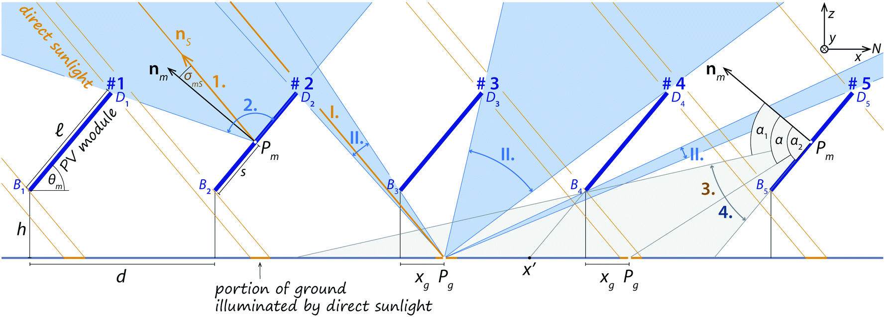 | ||
Fig. 1 Illustrating the geometrical configuration of a (periodic) PV field and the illumination components, which reach each module on the front. The modules are labeled with #1–#5. At #1, the geometrical parameters h,  , d and θm are illustrated – d is the horizontal length of a unit cell. At #2, the two irradiance components illuminating the module from the sky at Pm are indicated: 1. direct and 2. diffuse. Below #3, the I. direct and II. diffuse illumination of point Pg on the ground are illustrated – here diffuse illumination origins from three angular intervals. On #5 the angular range of light reaching Pm from the ground is indicated. It consists of 3. direct and 4. diffuse light being reflected from the ground. Components 1.–4. are summarized in Table 1. Here, we assume w.l.o.g. that the PV system is located on the northern hemisphere and oriented towards South. , d and θm are illustrated – d is the horizontal length of a unit cell. At #2, the two irradiance components illuminating the module from the sky at Pm are indicated: 1. direct and 2. diffuse. Below #3, the I. direct and II. diffuse illumination of point Pg on the ground are illustrated – here diffuse illumination origins from three angular intervals. On #5 the angular range of light reaching Pm from the ground is indicated. It consists of 3. direct and 4. diffuse light being reflected from the ground. Components 1.–4. are summarized in Table 1. Here, we assume w.l.o.g. that the PV system is located on the northern hemisphere and oriented towards South. | ||
The PV field is irradiated from direct sunlight under the Direct Normal Irradiance (DNI)§ and the direction nS, which is determined by the solar azimuth ϕS and the solar zenith θS. The latter is connected to the solar altitude aS (the height above the ground) via aS = 90° − θS. Further, the PV field receives diffuse light from the sky, which is given as Diffuse Horizontal Irradiance (DHI). However, for calculating the total irradiance onto the module, also light reflected from the ground and shadowing by the other modules must be taken into account.
Due to the typical geometry of a power plant the specular reflected DNI from the front side will seldom reach the back side of the front row. The diffuse reflectivity of the module should be significantly lower. In the current model we therefore assume the solar modules to be completely black and to not reflect any light. This might lead to a slight underestimation of the illumination.
Fig. 1 shows the different components of light, which can reach the front of a PV module at point Pm. The numbers 1.–4. correspond to the numbers in the figure – illumination on the sky is w.l.o.g. indicated for module #2 while illumination from the ground is indicated w.l.o.g. for module #5.
(1) Direct sunlight hits the modules under the direction nS. It leads to the irradiance component Iskydir,f(s) = DNIcosσmS, where s is the distance between the lower end of the module B2 and Pm,  , and σmS is the angle between the module surface normal and the direct incident sunlight.
(2) Diffuse skylight Iskydiff,f(s) hits the module at Pm from directions within the wedge determined by ∢D1PmD2. Diffuse light does not only reach the module from directions within the xz-plane but from a spherical wedge, which is closely linked to the sky view factor as for example used by Calcabrini et al.20
(3) Igr.dir,f(s) denotes direct sunlight that hits the module after it was reflected from the ground.
(4) Finally, Igr.diff,f(s) denotes diffuse skylight that hits the module after it was reflected from the ground.
All four components are summarized in Table 1. Table 2 denotes all parameters that are used as input to the model.
 . These components have to be considered for front and back sides – hence eight components in total. The numbers correspond to the numbers in Fig. 1
| 1. | Direct irradiance from the sky + circumsolar brightening | I skydir(s) |
| 2. | Diffuse irradiance from the sky | I skydiff(s) |
| 3. | Diffuse irradiance from the ground originating from direct sunlight + circumsolar brightening | I gr.dir(s) |
| 4. | Diffuse irradiance from the ground originating from diffuse skylight | I gr.diff(s) |
| a This parameter also can be spectral. Then, the unit would be W (m2 nm)−1. | |
|---|---|
| Module parameters (depicted in Fig. 1 ) | |

|
Module length (m) |
| w | Module width (m) |
| d | Module spacing (m) |
| h | Module height above the ground (m) |
| θ m | Module tilt angle |
|
|
| Solar parameters | |
| DNI | Direct normal irradiance (W m−2)a |
| DHI | Diffuse horizontal irradiance (W m−2)a |
| θ S | Zenith angle of the sun (connected to solar altitude aSvia aS = 90° − θS |
| ϕ S | Azimuth of the Sun |
| A | Albedo of the ground |
|
|
| Economical parameters | |
| c P | Peak power related system costs ($ per kWp) |
| c L | Land consumption related costs ($ per m2) |
The total irradiance (or intensity) on front is given by
| If(s) = Iskydir,f(s) + Iskydiff,f(s) + Igr.dir,f(s) + Igr.diff,f(s), | (1) |
As noted above, the incident light is given as DNI and DHI. The nonuniform irradiance distribution on the module front and back surfaces has to be considered.21,22 For the further treatment, it is therefore convenient to define unit-less geometrical distribution functions as for the components arising from direct sunlight and diffuse skylight, respectively. The geometrical distribution functions are closely related to the concept of view factors, which is often used for such illumination models.4,20,23 Usually, view factors are defined such that they describe the radiation from one area onto another area, hence they give the average radiation onto the area, e.g. a module. However, we do not seek the mean irradiation on a module but the minimal irradiation. This is because of the electric properties of PV modules, as described in Section 3.1.
 | (2) |
In eqn (2) we omitted the superscripts “sky” and “gr.”. The calculation of the components ιgr.dir,f(s) and ιgr.diff,f(s) requires the integration over geometrical distribution functions on the ground γdir(xg) and γdiff(xg), where xg is the coordinate of the point Pg on the ground.
In particular, we have where we omitted the subscripts “diff” and “dir”. The coordinate xg(s,α), on which γdir and γdiff are evaluated, is defined such that the angle between the line  and the module normal nm is equal to α – the integration parameter. In Fig. 1 the fractions of the ground, which are illuminated by direct sunlight, are marked in orange.
 | (3) |
Fig. 2 shows an example for illumination onto the ground: subfigure (a) illustrates the position of the solar modules #1 and #2. Subfigure (b) shows the geometrical distribution functions on the ground. γdiff is minimal below the module where the angle covered by the module is largest; and maximal at x′, because here the ground sees least shadow from module #1.
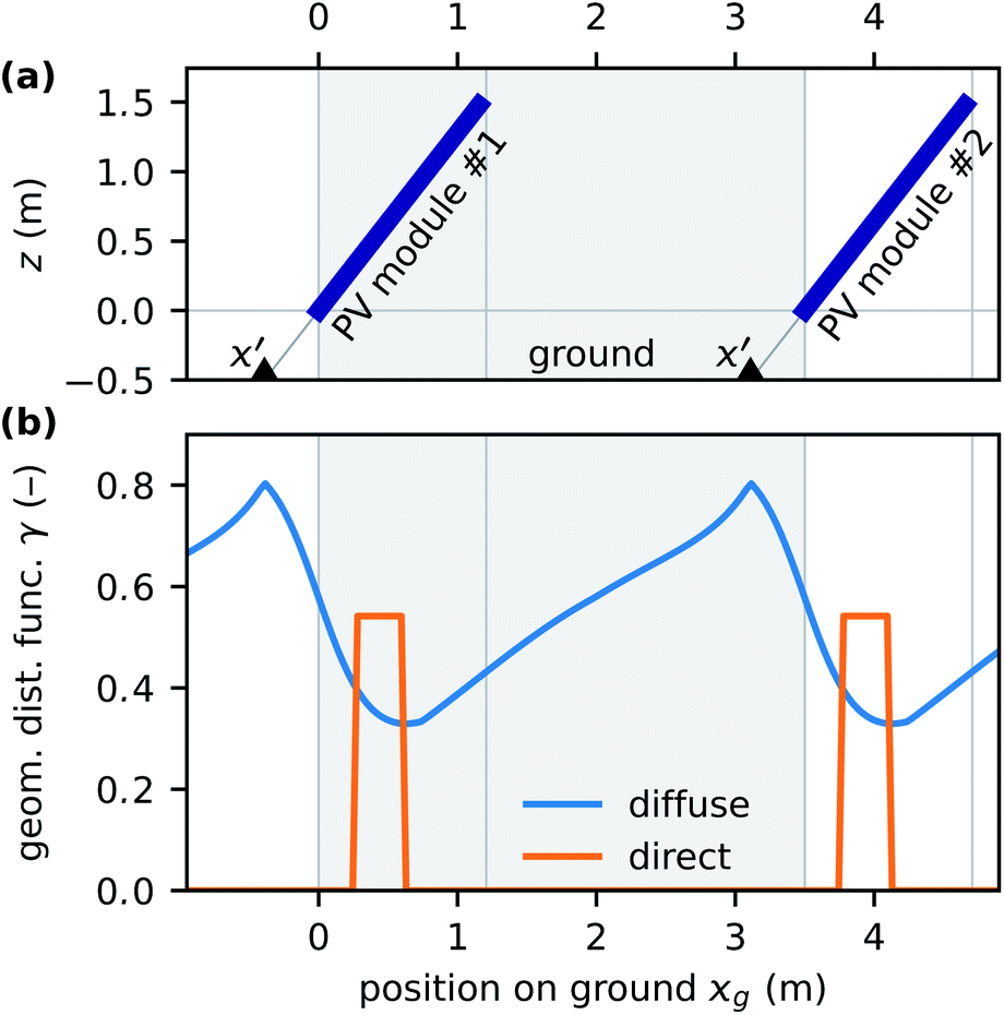 | ||
Fig. 2 An example for (a) a module configuration and (b) the corresponding diffuse and direct geometrical distribution functions at the ground γdiff and γdir. The following parameters were used:  = 1.96 m, d = 3.50 m, h = 0.50 m and θm = 52°. The solar position for the direct component was θS = 57.2° and ϕS = 143.3° (Berlin, 20 September 2019, 11:00 CEST). The unit cell is represented as shaded area. = 1.96 m, d = 3.50 m, h = 0.50 m and θm = 52°. The solar position for the direct component was θS = 57.2° and ϕS = 143.3° (Berlin, 20 September 2019, 11:00 CEST). The unit cell is represented as shaded area. | ||
Depending on the geometrical module parameters and the position of the Sun, the directly illuminated area (1) may lay completely within the unit cell as in the examples in Fig. 1 and 2, (2) it may extend from one unit cell into the next or (3) no direct light can reach the ground. The latter can occur when the module spacing d decreases or when the solar altitude aS is low.
Fig. 3 shows the eight geometrical distribution functions ι corresponding to the irradiance components hitting the PV module on its front and back sides. While the functions originating from the sky (a) are stronger on the front side, the components originating from the ground (b) are stronger on the back side. This can be understood by the opening angles: the opening angle towards the sky is larger on the front side, but the opening angle of the ground is larger at the back.
 | ||
Fig. 3 Geometrical distribution functions on the module for light the module receives (a) from the sky and (b) the ground. The following parameters were used:  = 1.96 m, d = 3.50 m, h = 0.50 m, θm = 52°, and albedo A = 30%. The solar position for the direct components was θS = 57.2° and ϕS = 143.3° (Berlin, 20 September 2019, 11:00 CEST). = 1.96 m, d = 3.50 m, h = 0.50 m, θm = 52°, and albedo A = 30%. The solar position for the direct components was θS = 57.2° and ϕS = 143.3° (Berlin, 20 September 2019, 11:00 CEST). | ||
All calculations presented in this work were performed with Python using numpy as numerical library for fast tensor operations.
3. Annual energy yield
3.1. Calculating the energy yield
We calculate the annual electrical energy yield EY by feeding the illumination model described in Section 2 with irradiance data. To demonstrate the features of the model, we use TMY3 (Typical Meteorological Year 3) data for this work. TMY3 data is well suited to estimate the solar energy yield for thousands of different locations.24 Amongst other parameters, the TMY3 data contain hourly DHI(t) and DNI(t) values. The overall EY given in [EY] = kW h per m² and year is the sum of the energy yields harvested over the course of a year at the module front and back sides, EY = EYf + EYb, which are calculated with | (4) |
The ι-functions are evaluated on the position  , where
  is the set of all considered positions along the module. In a conventional PV module, all cells are electrically connected in series and therefore the cell generating the lowest current limits the overall module current. To take this into account, we determine ŝi such that
| (If + Ib)(ŝi,ti) ≤ (If + Ib)(s,ti) | (5) |
 . This means that the position on the module with the lowest irradiance, which is proportional to the solar cell current, determines the overall module performance. For high-end solar modules, the module performance might be higher depending on how bypass diodes are implemented. Therefore, our condition establishes a lower bound of the module performance under certain illumination conditions.
To model the diffuse irradiance we use the Perez model, that is widely used for solar cell simulations. The Perez model distinguishes three different components of diffuse irradiance to calculate the intensity on a tilted plane: isotropic dome, circumsolar brightening and horizontal brightening. For modelling the illumination the circumsolar brightening component is added to the direct normal irradiance because it is centred at the position of the sun. The horizontal brightening is shaded by rows in front and back and is therefore not considered to calculate the final irradiance. For the isotropic dome irradiation on the module, the corresponding geometrical distribution functions ιdiff(s) need to be calculated only once.
For the components arising from direct sunlight, also the geometrical distribution functions ιdir(s,ti) are time-dependent, because they depend on the position of the Sun (θS,i, ϕS,i),¶ which we calculate using the Python package Pysolar.28
3.2. Results and discussion
As an example, we discuss results for two locations with different climates: first, Dallas/Fort Worth area, Texas (TX), USA (Denton, 195 m elevation, 33.21° N, 97.13° W) with a humid subtropical climate (Köppen–Geiger classification Cfa29) with hot, humid summers and cool winters. Secondly, Seattle, Washington (WA), USA (Boeing Field, 47.68° N, 122.25° W) with a warm-temperate (Mediterranean) climate (Köppen–Geiger classification Csb29) with relatively dry summers and cool wet winters. Fig. S1† shows climate diagrams for these two locations.In the ESI,† we also show results for Daggett, USA (Mojave desert, 585 m elevation, 34.87° N, 116.78° W) with a hot desert climate (Köppen–Geiger classification BWh29) and Havana, Cuba (Casa Blanca, 50 m elevation, 23.17° N, 82.35° W) with a tropical climate (Köppen–Geiger classification A29).
Fig. 4 shows the annual radiant exposure in (a) Dallas and (b) Seattle for bifacial PV modules (left) in a big PV field and the contributions from the front (middle) and back sides (right). The data shown in the figure are calculated like the energy yield according to eqn (4), where we set ηf = ηb = 1. We see that H generally increases with the module spacing. However, it is not economical to have a too large distance between the rows as we will see when considering the electricity cost in Section 4.
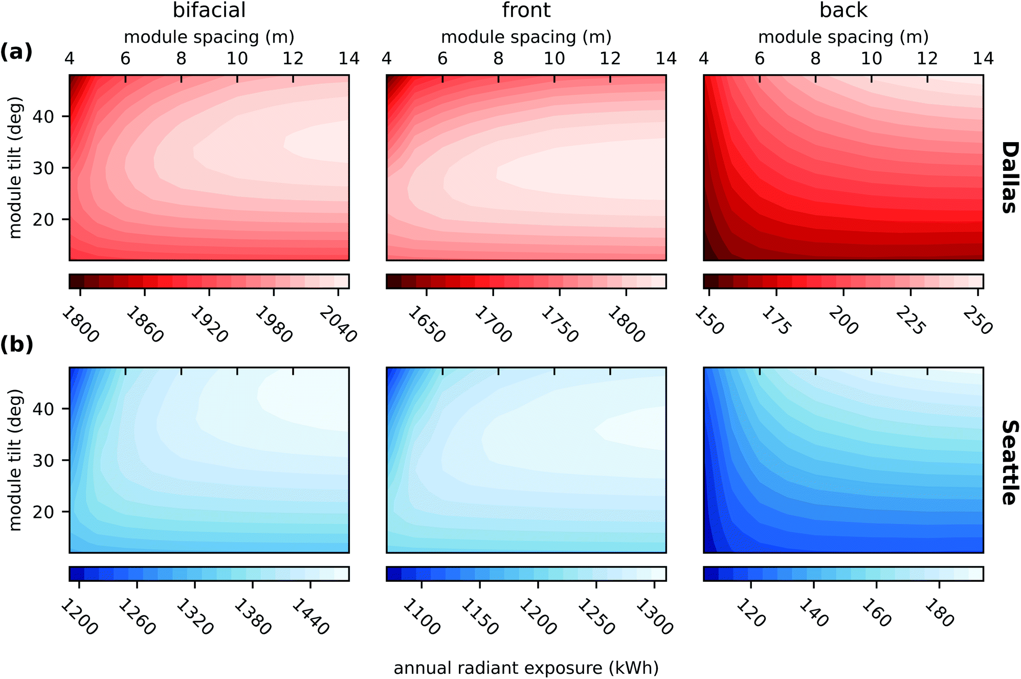 | ||
| Fig. 4 Annual radiant exposure for bifacial modules and the contributions from front and back sides in a large PV field as a function of module spacing d and module tilt θm. Results are shown for Dallas, TX, (top row) and Seattle, WA, (bottom row). The annual radiation yield is calculated using eqn (4) with ηf = ηb = 1. Simulated with m module height h = 0.5 m and albedo A = 30%. | ||
For Dallas, the optimal angle for monofacial modules, which only can utilize front illumination, is about 28°; it is mainly determined by direct sunlight. For back illumination, H increases significantly with the module inclination angle θm: hardly any direct light reaches the module at the back, but contributions from diffuse sky and reflected from the ground increase with θm. Increasing the module tilt further reduces the shaded area on the ground and therefore increases ground illumination. The optimal module tilt for a bifacial module is a compromise between the optimal tilt for the front and beneficial higher tilt angles for back contribution. Overall, the optimal module tilt for bifacial modules is significantly higher than for monofacial modules. Here it is about 36°.
Overall, the trends for Seattle are comparable to those for Dallas. However, we can identify differences: the overall radiant exposure is much lower because Seattle sees around 2170 annual Sun hours, compared to about 2850 h in Dallas.30 Further, the optimal tilt for monofacial and bifacial modules is 32° and 44°, respectively, which is explained by the higher latitude of Seattle.
For the front side illumination we see the interesting effect that, while the latitude of Seattle and Dallas differ by 14.5°, the respective optimal tilt angles only differ by 4°. This is probably because of the higher contribution on the annual radiant exposure from the summer months in Seattle compared to Dallas. While in Seattle May to September contribute 77% of the annual radiant exposure this is only 65% in Dallas. Because the module irradiance during the summer months (with higher elevation angles of the Sun) benefits from lower tilt angle θm values this can explain the difference of latitude to optimal tilt angles. The higher fraction of diffuse light in Seattle that also benefits the radiant exposure on the front side for small θm might additionally increase this effect.
Fig. 5 shows how much the different irradiation components contribute to the annual radiant exposure for a bifacial module with d = 10 m module spacing, θm = 34° tilt and albedo A = 30% in Dallas: about 74% of the total exposure arises from direct sunlight impinging onto the module front, 14% are due to diffuse skylight impinging onto the front but the fraction of light that reaches the front from the ground is almost negligible. However, of the 10.5% exposure received by the back, around 88% is reflected from the ground. Hence, the albedo only has little influence onto the energy yield of monofacial modules but is very relevant for bifacial modules. Fig. S4† shows corresponding results for Seattle. Compared to Dallas, Seattle shows 1.4% per larger contribution by the back side. While the front side receives radiation with a ratio of 3.5:1 of direct to diffuse light, for the back side, this ration is close to 1:1. These results show that four factors drive the gain of bifacial modules instead of monofacial modules: the albedo of the ground, the module tilt angle, the module spacing and the overall fraction of diffuse light.
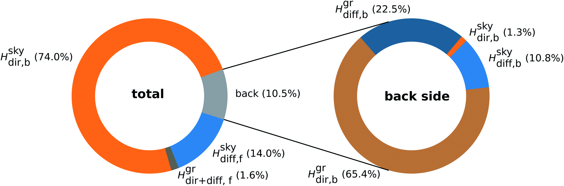 | ||
| Fig. 5 (left) Different annual radiant exposure components for a bifacial solar cell in Dallas. (right) Detailed picture for the back side. Simulated with module spacing d = 10 m, module tilt θm = 34° m, module height h = 0.5 m and albedo A = 30%. | ||
Also the mounting height h affects the bifacial gain. Increasing the mounting height monotonically raises the energy yield. Therefore it is difficult to optimise this parameter without knowing additional technical and commercial constraints. However, we find that the bifacial gain starts to saturate for a height above 0.5 m, which is in agreement with work from Kreinin et al.17 Since a mounting height of h = 0.5 m seems realistic all simulations in our work are performed with this mounting height.
4. Minimising the electricity cost
In Section 3 we discussed how to calculate the annual electrical energy yield and we analysed how the annual radiant exposure on the modules depends on the module spacing and tilt for two examples: Dallas and Seattle. In this section, we are going to derive a simple model for the electricity cost and perform some cost optimisations.4.1. Levelised cost of electricity
As a measure for the electricity cost we use the levelised cost of electricity (LCOE), which is a key metric for electricity generation facilities. In the simplest case, the LCOE is given as the total cost CF spent in the facility during its lifetime T (in years) divided by the total amount of electric energy Etotal generated in that time. Using the yield of a meteorological representative year allows to calculate the total yield by multiplying the annual power production with the lifetime of the facility.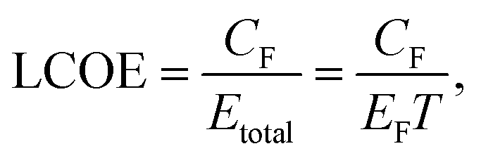 | (6) |
The total cost can be split into two components, associated with the peak power CP (including modules, inverters, mounting etc.) and the land consumption CL (lease, fences, cables etc.) of the facility.
| CF = CP + CL | (7) |
By considering a facility with a PV-field of M rows with N modules each the costs can be calculated per unit cell,
| CF = (CP,m + CL,m)MN. | (8) |
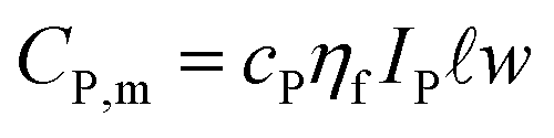
The peak-power related costs per module CP,m are calculated with
 | (9) |
 denote the module width and length, respectively. ηf denotes the power conversion efficiency on the front side of the solar cell.
The cost of land consumption per module depends on module width w and spacing d,
| CL,m = cLdw | (10) |
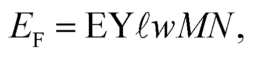
The annual generated electric energy of the PV field is given by with the annual yield EY according to eqn (4).
 | (11) |
Combining eqn (6)–(11) and simplifying leads to the expression which is independent of the field dimensions M and N and the module width w.
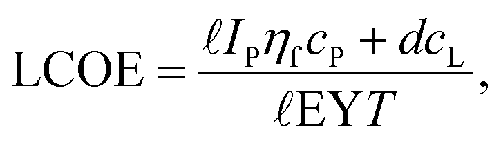 | (12) |
In this study, we assume for the overall costs of the PV system cm = 1000 $ per kWp, which includes all costs over the lifetime of the solar park, such as PV module investment, balance of system cost, planning, capital cost and others. The land cost is not included in this quantity. The lifetime is assumed to be T = 25 years, a typical time span for the power warranty of solar cell modules.27
In our optimisation, we aim to minimize the LCOE as parameter of the module spacing d and the solar module tilt θm. We perform the optimisation for five land-cost scenarios cL, in which we assume to include all costs that are related to an increase of area such as lease, cables, fences etc.Table 3 gives an overview of the cost scenarios and the resulting fraction of the land costs on the total costs, (CL/CF).
 = 1.96 m and ηf = 20%
| c P ($ per kWp) | c L ($ per m2) | C L/CF (%) |
|---|---|---|
| 1000 | 1.00 | 2.5 |
| 1000 | 2.50 | 6.0 |
| 1000 | 5.00 | 11.3 |
| 1000 | 10.00 | 20.3 |
| 1000 | 20.00 | 33.8 |
4.2. Optimisation method
As optimisation method we use Bayesian optimisation, which is well suited to find a global minimum of black box functions, which are expensive to evaluate.32 Bayesian optimisation has been used in a wide variety of applications such as robotics,33 hyper parameter tuning34 or physical systems.35,36In principle, Bayesian optimisation consists of two components: a surrogate model that approximates the black box function and its uncertainty (based on previously evaluated data points) and an acquisition function that determines the next query point from the surrogate model. After evaluating the function for the queried data point the surrogate model is updated and the next step can be computed with the acquisition function. This cycle is repeated until a specified number of steps or a convergences criteria is reached. We use the implementation from scikit-optimize with Gaussian process as surrogate model and expected improvement as acquisition function.37
4.3. Optimisation results
Traditionally, the optimal tilt and module spacing are often estimated with the winter solstice rule.38,39 The optimal distance between two rows of modules is defined as the shortest distance for which the shadow of a row of modules does not hit the next row of modules in a specified solar time window (e.g. 9 am–3 pm) on winter solstice. As a rule of thumb the tilt is often chosen to be equivalent to the latitude of the facility location. However these rules do not consider the economic trade off between land costs and energy yield or typical weather patterns (e.g. foggy winters) that vary for different locations.Fig. 6 and 7 shows the optimisation results for a field of (a) bifacial and (b) monofacial PV modules in Dallas and Seattle, respectively. Black dots mark evaluated data points, the red dot marks the found optimum and the color map shows the interpolation of the LCOE by the Gaussian process. The blue line indicates the winter solstice rule (9 am).
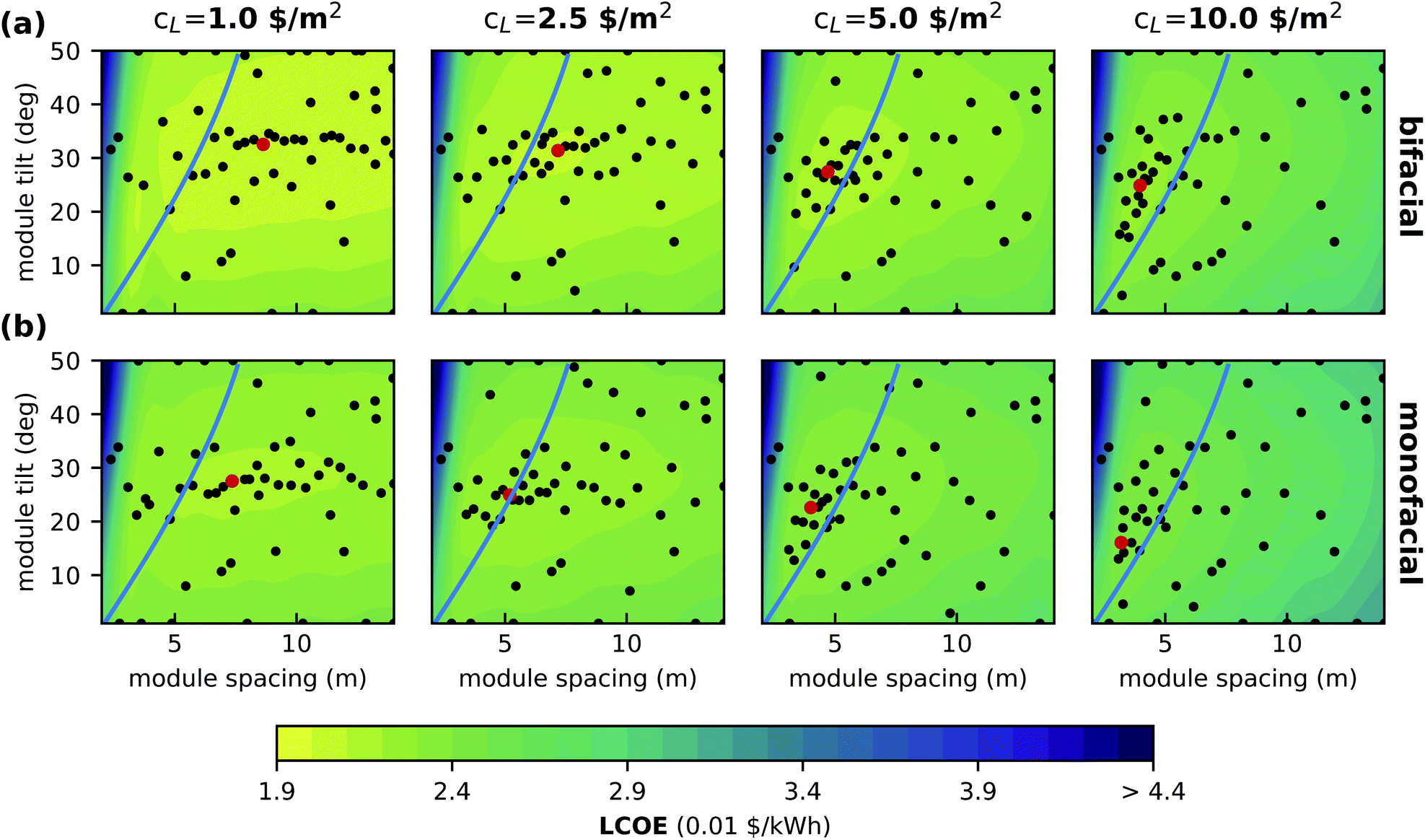 | ||
| Fig. 6 Results of the Bayesian optimisation for minimising LCOE of (a) bifacial and (b) monofacial PV modules in Dallas with the land cost cL scenarios 1, 2.5, 5, and 10 $ per m2. Black dots mark evaluated configurations and the color map corresponds to the interpolation by a Gaussian process. The red dot indicates the minimal LCOE found by the optimisation. The blue curves indicate rule-of-thumb module distance according to ‘no shadowing of neighboring modules at winter solstice’. Simulations with albedo A = 30%, module height h = 0.5 m and peak power costs cp = 1000 $ per kW h. | ||
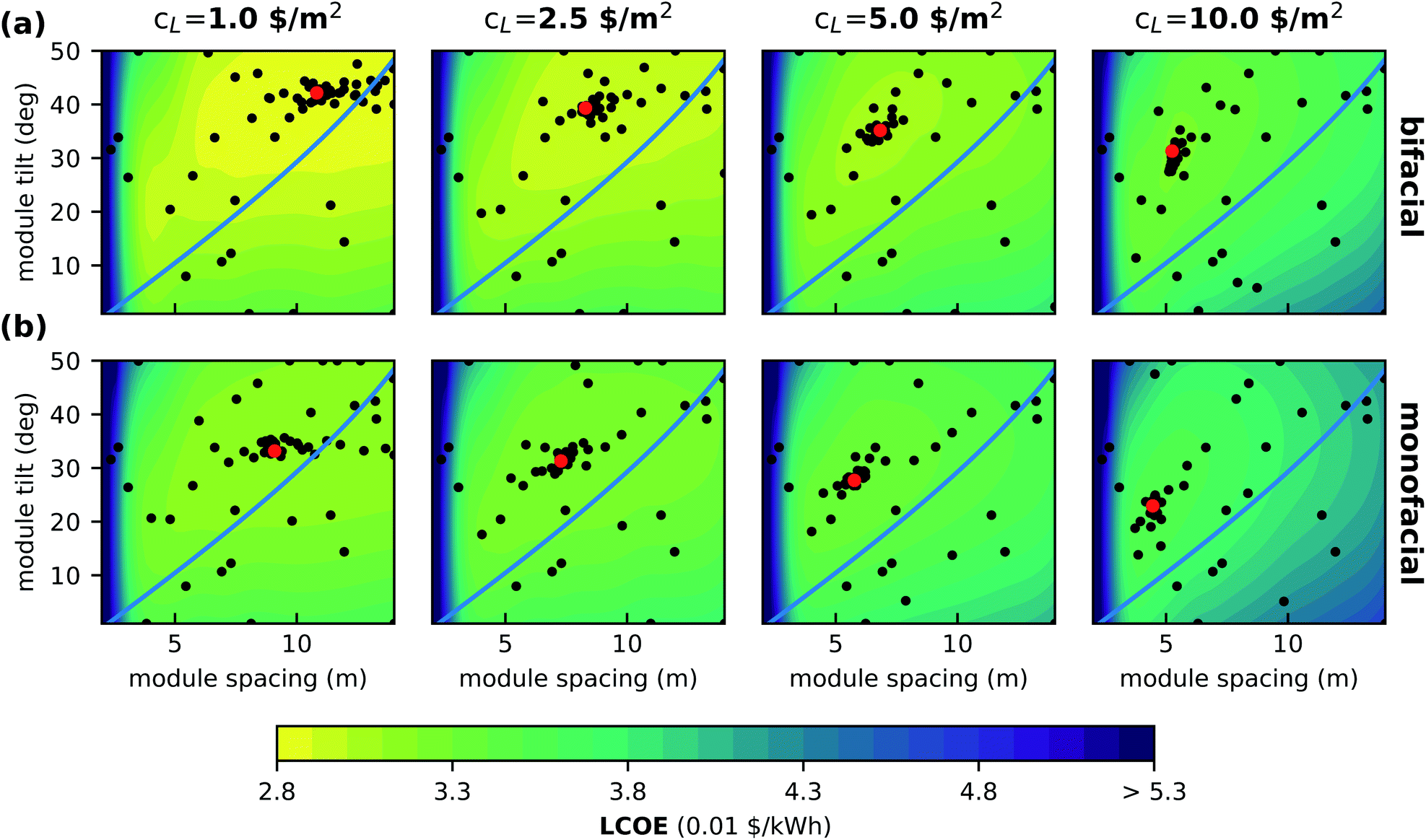 | ||
| Fig. 7 Results of the Bayesian optimisation for minimising LCOE of (a) bifacial and (b) monofacial PV modules in Seattle with the land cost cL scenarios 1, 2.5, 5 and 10 $ per m2. Black dots mark evaluated configurations and the color map corresponds to the interpolation by a Gaussian process. The red dot indicates the minimal LCOE found by the optimisation. The blue curves indicate rule-of-thumb module distance according to ‘no shadowing of neighboring modules at winter solstice’. Simulations with albedo A = 30%, module height h = 0.5 m and peak power costs cp = 1000 $ per kW h. | ||
We see that the optimum shifts to smaller module spacing with increasing land cost. Further, also the optimal module tilt decreases in order to compensate for increased shadowing because of less module spacing. Overall, bifacial installations show larger module spacing and higher tilt angles in optimal configurations compared to monofacial technology. With increasing land costs and therefore reduced optimal module spacing the cost landscape gets increasingly steep. The sensitivity of the optimised parameters increases and using non-optimal geometrical configurations results in increasing yield loss. Seattle shows the same trends for optimal configuration in different cost scenarios. Compared to Dallas optimal tilt and spacing are higher.
Our optimisation results differ significantly from the geometric parameters obtained from the winter solstice rule. For Dallas the winter solstice rule only provides comparable optimal parameters for cL = 5 $ per m2. In Seattle, the optimal distances are shorter and the optimal module tilts are larger than expected from the winter solstice rule for all cost scenarios. This can be understood when considering the large share of diffuse light during the Seattle winter, which mitigates shading losses significantly.
Table 4 compares the LCOE obtained from optimisation to results for rule-of-thumb geometries (tilt angle = latitude, distance according to 9 am winter solstice rule) for different land cost scenarios. Depending on the location and cost scenario we see a reduction of LCOE of up to 23%. The rule-of-thumb approach shows its weakness especially in Seattle. There is a general trend for higher reductions at high cost scenarios, where the cost landscape is increasingly steep (see Fig. 6 and 7). The optimisation for Havana in general exhibits the smallest reduction of LCOE but compared to the other locations there is no clear trend for higher reductions for higher land costs.
| c L ($ per m2) | LCOE (cents) optimised | Rule-of-thumb | Reduction (%) | |||||||||
|---|---|---|---|---|---|---|---|---|---|---|---|---|
| DALL. | HAVA. | MOJA. | SEAT. | DALL. | HAVA. | MOJA. | SEAT. | DALL. | HAVA. | MOJA. | SEAT. | |
| 1.0 | 2.04 | 1.84 | 1.57 | 2.83 | 2.05 | 1.87 | 1.58 | 2.85 | 0.5 | 1.6 | 0.6 | 0.7 |
| 2.5 | 2.10 | 1.89 | 1.61 | 2.93 | 2.10 | 1.89 | 1.62 | 3.00 | 0.0 | 0.0 | 0.6 | 2.3 |
| 5.0 | 2.17 | 1.94 | 1.67 | 3.07 | 2.18 | 1.94 | 1.68 | 3.24 | 0.5 | 0.0 | 0.6 | 5.2 |
| 10.0 | 2.28 | 2.02 | 1.77 | 3.28 | 2.33 | 2.04 | 1.80 | 3.74 | 2.1 | 1.0 | 1.7 | 12.3 |
| 20.0 | 2.47 | 2.17 | 1.92 | 3.62 | 2.63 | 2.23 | 2.06 | 4.73 | 6.1 | 2.7 | 6.8 | 23.5 |
From these results it is clear that the winter solstice rule is not able to properly reflect different economic trade-offs or different illumination conditions over the course of the year. This is especially true when setting the tilt angle to the latitude of the location. For a minimal LCOE module tilt and spacing should be optimised independently from each other. Further, typical weather patterns and the local economic situation must be taken into account.
4.4. Discussion
The results of all optimisations are summarised in Fig. 8 and Table 5. We see that the optimal LCOE increases slightly with the land cost. Further, in Seattle the LCOE difference between mono- and bifacial modules is larger as in Dallas, Havana or the Mojave Desert. This is caused by the larger module tilt and diffuse light share in Seattle, which increases the fraction of illumination at the module back. Dallas and the Mojave Desert have comparable latitude but show a small difference in bifacial gain due to the higher diffuse light share in Dallas. As discussed above, the optimal module tilt decreases with increased land consumption cost cL.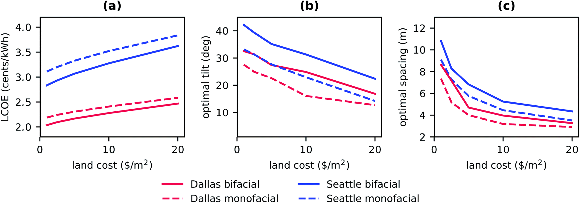 | ||
| Fig. 8 Results of the optimisation for different land cost scenarios in Dallas (red lines) and Seattle (blue lines): (a) lowest LCOE and (b) optimal module tilt and (c) optimal spacing. Simulations with albedo A = 30%, module height h = 0.5 m and peak power costs cp 1000 $ per kW h. | ||
| c L ($ per m2) | C L/CF (%) | d (m) | Bif. gain (%) | |||||||||
|---|---|---|---|---|---|---|---|---|---|---|---|---|
| DALL. | HAVA. | MOJA. | SEAT. | DALL. | HAVA. | MOJA. | SEAT. | DALL. | HAVA. | MOJA. | SEAT. | |
| 1.0 | 2.2 | 2.0 | 2.1 | 2.7 | 8.6 | 8.2 | 8.5 | 10.8 | 11.4 | 11.3 | 10.7 | 13.6 |
| 2.5 | 4.4 | 3.3 | 4.2 | 5.0 | 7.2 | 5.3 | 6.9 | 8.3 | 11.0 | 10.1 | 10.3 | 12.7 |
| 5.0 | 5.7 | 4.7 | 6.1 | 8.0 | 4.7 | 3.9 | 5.1 | 6.8 | 9.6 | 9.0 | 9.4 | 11.7 |
| 10.0 | 9.2 | 7.8 | 9.6 | 11.8 | 4.0 | 3.3 | 4.2 | 5.2 | 8.8 | 7.9 | 8.4 | 10.5 |
| 20.0 | 14.3 | 13.9 | 15.1 | 18.2 | 3.3 | 3.2 | 3.5 | 4.3 | 7.3 | 7.5 | 7.3 | 9.2 |
In general, we see that for a utility scale solar cell plant both, the module tilt and the distance between rows, affect the annual energy yield. Increasing the distance increases the energy yield and the costs per module while tilt can be optimised cost-neutral. The optimal distance between rows is a compromise between increasing costs with higher land use for higher distances and lower energy yield due to shading for lower distances. This is true also for monofacial modules but due to the increased relevance of light reflected from the ground it is more relevant for bifacial modules.
The optimal configuration for bifacial solar cells depends on the radiation conditions and the albedo of the facility location. With increasing latitude (and therefore lower solar elevation angles), albedo and diffuse light contribution the bifacial gain will be increased and therefore make this type of PV technology more attractive for utility scale developers.
Cost optimisations for PV installation are quickly outdated because PV module prices have been decreasing for many years and land cost is very volatile. However the optimal installation geometry only depends on the ratio of land cost related to total costs and not absolute values. Hence, at a scenario of cL = 10 $ per m2 and cP = 1500 $ per kWp yields the same optimisation result as cL = 5 $ per m2 and cP = 750 $ per kWp.
5. Conclusions
We developed a detailed model to calculate the irradiation onto both sides of a PV module, which is located in a large PV field. With this model, we could estimate the annual energy yield for monofacial and bifacial PV modules as a function of the module spacing and the module tilt. We assume a constant power conversion efficiency and a simple approach to calculate the levelised cost of electricity allowing for a technology independent modeling. Combined with a Bayesian optimisation algorithm, this allowed us to minimise the LCOE as a function of module spacing and module tilt for different land consumption costs. Due to the general approach the presented LCOE have the character of an example. It can be refined by implementation of module specific derating factors such as the temperature and incident angle dependent conversion efficiency behaviour.Our results basically show that the bifacial gain and optimal geometry depend on the specific location and cost scenario. The bifacial gain can be expected to increase for locations with higher latitude and higher diffuse light share.
The usually used rule of thumb, no shadowing at winter-solstice and module tilt angle equal to the geographical latitude, leads to suboptimal module spacing and tilt combinations, because it does not account for economic trade-offs and the influence of the local climate. In contrast, optimising the parameters in Seattle can lead to a 23% reduction of LCOE for high land cost scenarios. This shows the significance of site-specific and land-cost dependent optimisation and helps users to identify the configurations yielding minimal LCOE.
Conflicts of interest
There are no conflicts to declare.Acknowledgements
We thank Lev Kreinin and Asher Karsenti from SolAround for fruitful discussions regarding the illumination model for bifacial solar cells. P. T. thanks the Helmholtz Einstein International Berlin Research School in Data Science (HEIBRiDS) for funding. The results were obtained at the Berlin Joint Lab for Optical Simulations for Energy Research (BerOSE) and the Helmholtz Excellence Cluster SOLARMATH of Helmholtz-Zentrum Berlin für Materialien und Energie, Zuse Institute Berlin and Freie Universität Berlin.Notes and references
- K. Yoshikawa, H. Kawasaki, W. Yoshida, T. Irie, K. Konishi, K. Nakano, T. Uto, D. Adachi, M. Kanematsu, H. Uzu and K. Yamamoto, Nat. Energy, 2017, 2, 17032 CrossRef CAS.
- A. Richter, M. Hermle and S. W. Glunz, IEEE J. Photovoltaics, 2013, 3, 1184–1191 Search PubMed.
- R. Kopecek and J. Libal, Nat. Energy, 2018, 3, 443–446 CrossRef.
- T. S. Liang, M. Pravettoni, C. Deline, J. S. Stein, R. Kopecek, J. P. Singh, W. Luo, Y. Wang, A. G. Aberle and Y. S. Khoo, Energy Environ. Sci., 2019, 12, 116–148 RSC.
- S. Chunduri and M. Schmela, Bifacial Solar Technology Report 2018 Edition, Taiyang news technical report, 2018 Search PubMed.
- Sanyo, Sanyo Canada launches first bifacial solar module -, 2009, https://www.greenlaunches.com/alternative-energy/sanyo-canada-launches-first-bifacial-solar-module.php Search PubMed.
- Yingli, Yingli's PANDA BIFACIAL Module Became the World's First Bifacial Module Certified by CGC, UL, and TUV Rheinland, 2018, http://ir.yinglisolar.com/news-releases/news-release-details/yinglis-panda-bifacial-module-became-worlds-first-bifacial Search PubMed.
- bSolar, bSolar launches High-Efficiency Bifacial Silicon Solar Cells, 2012, https://www.photovoltaik.eu/article-449463-30021/bsolar-launches-high-efficiency-bifacial-silicon-solar-cells-.html Search PubMed.
- TrinaSolar, Trina Solar to launch N-type i-TOPCon double-glass bifacial modules, 2019, https://solarpv.expert/2019/06/14/trina-solar-to-launch-n-type-i-topcon-double-glass-bifacial-modules/ Search PubMed.
- ITRPV, 10th Edition of the International Technology Roadmap Photovoltaics, Vdma technical report, 2019 Search PubMed.
- N. Ishikawa and S. Nishiyama, presented at the 3rd Bifi PV Workshop, Miyazaki, Japan, 2016 Search PubMed.
- F. Fertig, S. Nold, N. Wöhrle, J. Greulich, I. Hädrich, K. Krauß, M. Mittag, D. Biro, S. Rein and R. Preu, Prog. Photovoltaics Res. Appl., 2016, 24, 800–817 CrossRef.
- J. Appelbaum, Renewable Energy, 2016, 85, 338–343 CrossRef.
- M. R. Khan, E. Sakr, X. Sun, P. Bermel and M. A. Alam, Appl. Energy, 2019, 241, 592–598 CrossRef.
- I. Shoukry, J. Libal, R. Kopecek, E. Wefringhaus and J. Werner, Energy Procedia, 2016, 92, 600–608 CrossRef.
- M. T. Patel, M. R. Khan, X. Sun and M. A. Alam, Appl. Energy, 2019, 247, 467–479 CrossRef.
- L. Kreinin, A. Karsenty, D. Grobgeld and N. Eisenberg, 2016 IEEE 43rd Photovoltaic Specialists Conference (PVSC), 2016, pp. 2688–2691 Search PubMed.
- P. Grana, The new rules for latitude and solar system design, 2018, https://www.solarpowerworldonline.com/2018/08/new-rules-for-latitude-and-solar-system-design/ Search PubMed.
- B. Marion, S. MacAlpine, C. Deline, A. Asgharzadeh, F. Toor, D. Riley, J. Stein and C. Hansen, 2017 IEEE 44th Photovoltaic Specialist Conference (PVSC), 2017 Search PubMed.
- A. Calcabrini, H. Ziar, O. Isabella and M. Zeman, Nat. Energy, 2019, 4, 206–215 CrossRef.
- U. A. Yusufoglu, T. M. Pletzer, L. J. Koduvelikulathu, C. Comparotto, R. Kopecek and H. Kurz, IEEE J. Photovoltaics, 2015, 5, 320–328 Search PubMed.
- L. Kreinin, N. Bordin, A. Karsenty, A. Drori, D. Grobgeld and N. Eisenberg, 2010 35th IEEE Photovoltaic Specialists Conference, 2010, pp. 002171–002175 Search PubMed.
- X. Sun, M. R. Khan, C. Deline and M. A. Alam, Appl. Energy, 2018, 212, 1601–1610 CrossRef.
- S. Wilcox and W. Marion, Users manual for TMY3 data sets, National Renewable Energy Laboratory Technical Report NREL/TP-581-43156, National Renewable Energy Laboratory Golden, CO, 2008 Search PubMed.
- N. Martín and J. M. Ruiz, Prog. Photovoltaics Res. Appl., 2005, 13, 75–84 CrossRef.
- M. Jazayeri, S. Uysal and K. Jazayeri, 2013 High Capacity Optical Networks and Emerging/Enabling Technologies, 2013, pp. 44–50 Search PubMed.
- A. H. M. Smets, K. Jäger, O. Isabella, R. A. C. M. M. van Swaaij and M. Zeman, Solar energy: The physics and engineering of photovoltaic conversion technologies and systems, UIT Cambridge, 2016 Search PubMed.
- B. Stafford, Pysolar, 2018, DOI:10.5281/zenodo.1461066.
- M. Kottek, J. Grieser, C. Beck, B. Rudolf and F. Rubel, Meteorol. Z., 2006, 15, 259–263 CrossRef.
- L. Ozborn, Average Annual Sunshine in American Cities, 2019, https://www.currentresults.com/Weather/US/average-annual-sunshine-by-city.php Search PubMed.
- ISO 9845-1:1992, International organization for standardization technical report, 1992 Search PubMed.
- B. Shahriari, K. Swersky, Z. Wang, R. P. Adams and N. de Freitas, Proc. IEEE, 2016, 104, 148–175 Search PubMed.
- A. Cully, J. Clune, D. Tarapore and J.-B. Mouret, Nature, 2015, 521, 503–507 CrossRef CAS PubMed.
- J. Snoek, H. Larochelle and R. P. Adams, Practical Bayesian Optimization of Machine Learning Algorithms, 2012, http://papers.nips.cc/paper/4522-practical-bayesian-optimization Search PubMed.
- P.-I. Schneider, X. G. Santiago, C. Rockstuhl and S. Burger, Proc. SPIE, 2017, 103350, 103350O Search PubMed.
- H. C. Herbol, W. Hu, P. Frazier, P. Clancy and M. Poloczek, npj Comput. Mater., 2018, 4, 51 CrossRef.
- T. Head, MechCoder, G. Louppe, I. Shcherbatyi, Fcharras, Z. Vinícius, Cmmalone, C. Schröder, Nel215, N. Campos, T. Young, S. Cereda, T. Fan, Rene-Rex, Kejia (KJ) Shi, J. Schwabedal, Carlosdanielcsantos, Hvass-Labs, M. Pak, F. Callaway, L. Estève, L. Besson, M. Cherti, K. Pfannschmidt, F. Linzberger, C. Cauet, A. Gut, A. Mueller and A. Fabisch, Scikit-Optimize/Scikit-Optimize: V0.5.2, 2018, DOI:10.5281/zenodo.1207017.
- M. T. Patel, M. R. Khan, X. Sun and M. A. Alam, Appl. Energy, 2019, 247, 467–479 CrossRef.
- S. Sánchez-Carbajal and P. M. Rodrigo, Int. J. Photoenergy, 2019, 2019, 1–14 CrossRef.
Footnotes |
| † Electronic supplementary information (ESI) available. See DOI: 10.1039/c9se00750d |
| ‡ These authors contributed equally to this work. |
| § The irradiance or intensity is the radiant power a surface receives per area. |
| ¶ See for example ref. 27, appendix E. |
| || See for example ref. 27, chapter 21. |
| This journal is © The Royal Society of Chemistry 2020 |