
 Open Access Article
 This Open Access Article is licensed under a Creative Commons Attribution-Non Commercial 3.0 Unported Licence
Fast predictions of liquid-phase acid-catalyzed reaction rates using molecular dynamics simulations and convolutional neural networks†
Alex K.
Chew
 ab,
Shengli
Jiang
a,
Weiqi
Zhang
a,
Victor M.
Zavala
a and
Reid C.
Van Lehn
*ab
ab,
Shengli
Jiang
a,
Weiqi
Zhang
a,
Victor M.
Zavala
a and
Reid C.
Van Lehn
*ab
aDepartment of Chemical and Biological Engineering, University of Wisconsin-Madison, Madison, WI 53706, USA. E-mail: vanlehn@wisc.edu
bDOE Great Lakes Bioenergy Research Center, University of Wisconsin-Madison, Madison, WI 53706, USA
First published on 19th October 2020
Abstract
The rates of liquid-phase, acid-catalyzed reactions relevant to the upgrading of biomass into high-value chemicals are highly sensitive to solvent composition and identifying suitable solvent mixtures is theoretically and experimentally challenging. We show that the complex atomistic configurations of reactant–solvent environments generated by classical molecular dynamics simulations can be exploited by 3D convolutional neural networks to enable accurate predictions of Brønsted acid-catalyzed reaction rates for model biomass compounds. We develop a 3D convolutional neural network, which we call SolventNet, and train it to predict acid-catalyzed reaction rates using experimental reaction data and corresponding molecular dynamics simulation data for seven biomass-derived oxygenates in water–cosolvent mixtures. We show that SolventNet can predict reaction rates for additional reactants and solvent systems an order of magnitude faster than prior simulation methods. This combination of machine learning with molecular dynamics enables the rapid, high-throughput screening of solvent systems and identification of improved biomass conversion conditions.
Introduction
The catalytic conversion of lignocellulosic biomass is a promising strategy to obtain transportation fuels and high-value chemicals from renewable feedstocks.1 The conversion of biomass-derived molecules is typically facilitated by liquid-phase, acid-catalyzed reactions (examples shown in Fig. 1a) that are hindered by low reactivity in aqueous solution. One method to increase acid-catalyzed reaction rates is to modify the solvent composition by mixing organic, polar aprotic cosolvents with water to create mixed-solvent environments; such environments have been shown to improve reaction rates up to 100-fold compared to rates for the same reactions in pure water.2–4 Unfortunately, identifying solvent environments that improve reaction rates by trial-and-error experimentation is time-consuming, costly, and provides limited insight into the physical basis of solvent effects. Instead, computational tools have been applied to understand solvent effects on chemical reactivity and guide the design of solvent mixtures for efficient biomass conversion processes.5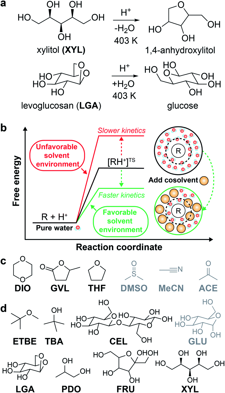 | ||
| Fig. 1 Overview of solvent effects on acid-catalyzed reactions and model systems. (a) Two example acid-catalyzed reactions: xylitol (XYL) dehydration and levoglucosan (LGA) hydrolysis. (b) Hypothesized effect of mixed-solvent environments on the free energy landscape of acid-catalyzed reactions. The schematic illustrates the formation of a local solvent domain (within the circular dashed line) around the reactant in a mixed-solvent environment that modifies the reaction free energy landscape, thus affecting reaction kinetics.3,4 (c) Organic, polar aprotic cosolvents modeled in this study, including dioxane (DIO), γ-valerolactone (GVL), tetrahydrofuran (THF), dimethyl sulfoxide (DMSO), acetonitrile (MeCN), and acetone (ACE). Molecules drawn in black were included in the training set. Molecules drawn in gray were included in the test set. (d) Biomass-derived model reactants modeled in this study, including ethyl tert-butyl ether (ETBE), tert-butanol (TBA), cellobiose (CEL), glucose (GLU), LGA, 1,2-propanediol (PDO), fructose (FRU), and XYL. The color scheme follows part (c), except TBA, PDO, and FRU were included as part of some of the reactant–solvent combinations in both training and test sets. | ||
In the past decade, ab initio quantum chemical methods have been used to quantify solvent effects on barriers to elementary steps for biomass conversion reactions.1,5,6 Using ab initio molecular dynamics (MD) simulations, Mellmer et al. found that the inclusion of organic cosolvents increases biomass conversion reaction kinetics by lowering the activation energy due to changes to the solvation environment around the acidic proton catalyst, the reactant, and charged transition states (Fig. 1b).3 The simulations revealed that hydrophilic reactants drive the formation of water-enriched local domains in mixed-solvent environments that preferentially solvate the acid catalyst and stabilize subsequent carbocation-like transition states.2–4 These findings suggest that the extent of water enrichment around the reactant is directly correlated with acid-catalyzed reaction performance. Similar studies have used ab initio techniques to understand how the solvent environment alters reaction kinetics for key acid-catalyzed reactions,5,7 such as the conversion of fructose to afford 5-hydroxymethylfurfural8,9 (a platform chemical for polymer precursors and transportation fuels).10 Unfortunately, while ab initio methods can directly probe mechanistic details of reactions, their high computational expense renders the screening of multiple solvent compositions infeasible.
Relative to ab initio MD, classical MD simulations can access longer timescales (μs) and larger length scales (nm) with significantly reduced computational budgets, allowing a more rapid characterization of complex solvent environments around even large reactants.11–13 Classical MD simulations are suitable for modeling the spatial organization of mixed-solvent environments that emerges from the interplay of reactant–solvent–cosolvent interactions and may impact reaction kinetics (e.g., due to preferential solvation of the reactant as described above) but may not be captured by bulk solvent descriptors (e.g., the dielectric constant).5,14 On the other hand, a key limitation of classical MD simulations is their inability to directly model chemical reactions. Nonetheless, we recently utilized classical MD simulations to understand and predict solvent effects on experimental reaction rates for the conversion of biomass-derived model compounds in aqueous mixtures of 1,4-dioxane (DIO), γ-valerolactone (GVL), and tetrahydrofuran (THF).4 Based on the hypothesis that classical MD simulations could quantify the reactant–water–cosolvent interactions that dictated reactivity in prior ab initio simulations,3 we developed an MD model consisting of only reactant, water, and cosolvent molecules and calculated three simulation-derived descriptors that quantified the extent of water-enrichment around the reactant, reactant–water hydrogen bonding, and reactant hydrophilicity. We then derived a linear regression model that used these three descriptors to predict experimental reaction rates and found good agreement in DIO–water mixtures.4 These findings showed that classical MD simulations can be used to predict solvent effects on reaction rates without explicitly modeling the acid catalyst or the reaction mechanism. The regression model was less accurate for GVL– and THF–water mixtures, indicating that either descriptors computed with classical MD cannot quantify reaction rates in these systems or that more complex descriptors must be defined to capture reactivity trends. However, designing new descriptors of reaction kinetics based on human intuition is challenging, often requiring complex and time-consuming data analysis tools (e.g. solvation free energies14,15 or three-dimensional solvent mapping12,14) that cannot be readily generalized across a range of solvent compositions.
As an alternative to designing descriptors via human intuition, machine learning methods have been increasingly used to infer molecular properties by automatically extracting features from complex sources of data.16–22 For example, convolutional neural networks (CNNs) can be used to identify and quantify patterns within two-dimensional (2D) spatial datasets such as images.23 By training on a suitable set of labeled image data, CNNs extract spatial features without requiring human supervision and can then utilize these features to classify image contents. CNNs have been shown to outperform other machine learning methods (e.g. fully connected neural networks and support vector machines)24 in the ImageNet Large-Scale Visual Recognition Challenge,25 a contest requiring a model to classify more than 1.2 million images. CNNs can be further generalized to extract features from three-dimensional (3D) volumetric data,26 which can facilitate the analysis of 3D molecular structures. For example, 3D CNNs have recently been used to detect protein functional sites,27 evaluate protein–ligand binding sites,28 and quantify protein–ligand binding affinities29 by training on protein database structures. Based on these examples and our prior success using classical MD simulations to predict acid-catalyzed reaction outcomes,4,14 we hypothesize that 3D CNNs can exploit the output of classical MD simulations to more accurately predict solvent effects on acid-catalyzed reaction rates.
In this work, we developed 3D CNNs that utilize information on atomic positions obtained from classical MD simulation trajectories to predict the rates of liquid-phase, acid-catalyzed biomass conversion reactions in mixed-solvent environments. To develop our training procedure, we use 76 experimentally determined reaction rates for 7 biomass-derived model reactants in DIO–, GVL–, and THF–water solvent mixtures as labels. For each experimental reaction rate and associated solvent mixture, we record configurations from a corresponding MD simulation trajectory (each configuration contains the 3D positions of atoms in reactant, solvent, and water molecules). Configurations collected from the simulation and their spatial rotations are used to obtain multiple voxel representations that map to the same experimental reaction rate and are used as input data for the 3D CNN. This procedure allows us to construct a rich training dataset that consists of 18![[thin space (1/6-em)]](https://www.rsc.org/images/entities/char_2009.gif) 240 voxel representations (over 240 distinct voxel representations mapping to each of the 76 experimental reaction rates). This approach seeks to demonstrate that MD trajectory data embeds rich information that explains reaction rates and that develops early in the MD simulation to drastically reduce computational time. We find that all 3D CNNs considered – including a new 3D CNN that we developed, which we call SolventNet, and two previously developed 3D CNNs (ORION30 and VoxNet31) – predict experimental reaction rates more accurately than models based on human-selected, MD-derived descriptors.4 SolventNet predictions generalize to a test set consisting of 32 experimentally determined reaction rates obtained from the literature, including rates for reactants in three additional polar aprotic cosolvents not included in model training – dimethyl sulfoxide, acetonitrile, and acetone – with distinct properties (e.g., functional groups, basicity, and polarizability) from the cosolvents used to train the model. We further find that accurate reaction rate predictions with SolventNet require as little as 4 ns of classical MD trajectory data, a 50-fold improvement from the original 205 ns of MD data used in models based on human-selected descriptors.4 We thus conclude that 3D atomistic configurations contain significant information that explains reaction rates and that such configurations develop early in the MD simulation. We envision that the computational efficiency associated with the combination of 3D CNNs and classical MD simulations will enable the integration of these tools with process models to screen solvents and optimize reactor conditions for biomass conversion processes.32
240 voxel representations (over 240 distinct voxel representations mapping to each of the 76 experimental reaction rates). This approach seeks to demonstrate that MD trajectory data embeds rich information that explains reaction rates and that develops early in the MD simulation to drastically reduce computational time. We find that all 3D CNNs considered – including a new 3D CNN that we developed, which we call SolventNet, and two previously developed 3D CNNs (ORION30 and VoxNet31) – predict experimental reaction rates more accurately than models based on human-selected, MD-derived descriptors.4 SolventNet predictions generalize to a test set consisting of 32 experimentally determined reaction rates obtained from the literature, including rates for reactants in three additional polar aprotic cosolvents not included in model training – dimethyl sulfoxide, acetonitrile, and acetone – with distinct properties (e.g., functional groups, basicity, and polarizability) from the cosolvents used to train the model. We further find that accurate reaction rate predictions with SolventNet require as little as 4 ns of classical MD trajectory data, a 50-fold improvement from the original 205 ns of MD data used in models based on human-selected descriptors.4 We thus conclude that 3D atomistic configurations contain significant information that explains reaction rates and that such configurations develop early in the MD simulation. We envision that the computational efficiency associated with the combination of 3D CNNs and classical MD simulations will enable the integration of these tools with process models to screen solvents and optimize reactor conditions for biomass conversion processes.32
The manuscript is organized as follows. We first describe the set of 108 experimentally determined reaction rates, each associated with a unique combination of reactant and mixed-solvent environment, that are used as labels for the training set (76 reaction rates) and test set (32 reaction rates). We then describe the training and validation of baseline linear and nonlinear models using data consisting of human-selected descriptors computed from MD trajectories, with one trajectory and corresponding set of descriptors per label. We next describe an alternative input data set generated by splitting each MD trajectory into 10 independent voxel representations for interpretation by 3D CNNs. After data augmentation, this procedure yields 240 voxel representations per label that are used to train and validate 3D CNNs for comparison to the baseline models. We then assess the test set and leave-one-out cross-validation accuracy of SolventNet to establish model generalizability. Finally, we visualize spatial features that influence SolventNet accuracy using saliency maps.
Results and discussion
Experimental reaction data used for model training and testing
A total of 108 previously reported, experimentally determined reaction rates for acid-catalyzed dehydration or hydrolysis reactions in mixed-solvent environments were used as labels for the training and testing of predictive models for acid-catalyzed reaction rates. Each reaction rate was measured for a unique reactant–solvent combination (i.e., a reactant in a mixed-solvent environment). A total of 76 experimental reaction rates (70% of the labels) were taken from ref. 4 and used as labels for the training set. The training set includes rates for 7 biomass-relevant model reactants: ethyl tert-butyl ether (ETBE), tert-butanol (TBA), 1,2-propanediol (PDO), levoglucosan (LGA), fructose (FRU), cellobiose (CEL), and xylitol (XYL). Solvent systems include aqueous mixtures with 25 wt%, 50 wt%, 75 wt%, or 90 wt% of one of three polar aprotic cosolvents: 1,4-dioxane (DIO), γ-valerolactone (GVL), and tetrahydrofuran (THF). 32 experimental reaction rates (30% of the labels) were taken from ref. 3 and 33 and used as labels for the test set. The test set includes rates for 4 model reactants: TBA, FRU, PDO, and glucose (GLU). Solvent systems include aqueous mixtures with dimethyl sulfoxide (DMSO), acetonitrile (MeCN), and acetone (ACE). Training set experiments were performed at temperatures between 343–433 K and test set experiments were performed at temperatures between 363–433 K. All experiments used triflic acid as a catalyst, except for test set experiments from ref. 33 (for FRU and GLU in aqueous mixtures of ACE) which used hydrochloric acid. The test set labels thus consist of independent reaction rates from different literature sources for reactants and cosolvents not included in the training set but at comparable experimental conditions. Chemical structures of all reactants and cosolvents are shown in Fig. 1c and d, respectively. Tables S1 and S2† list the reaction conditions for each label.To compare the effect of the mixed-solvent environment on reaction rates in different systems, eqn (1) defines the kinetic solvent parameter (σ) as the log-ratio between the apparent rate constant for the dehydration or hydrolysis of reactant r in a given mixed-solvent environment (krorg) and the apparent rate constant for the same reaction in pure water (kH2rO):4
 | (1) |
Baseline prediction models for reaction rates using human-selected descriptors from classical MD
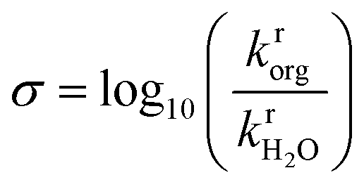
In prior work, we performed classical MD simulations of one reactant molecule in a mixed-solvent environment to generate a single 205 ns simulation trajectory for each of the 76 reactant–solvent combinations included in the training set.4Fig. 2a illustrates the general approach for extracting descriptors from these MD simulations to predict experimental kinetic solvent parameters. From each MD trajectory, we computed three physically motivated, human-selected descriptors that capture reactant hydrophilicity and solvent interactions: the preferential exclusion coefficient (Γ), which quantifies the local enrichment of water in the spatial region near the reactant; the hydrogen bonding lifetime between the reactant and water (τ), which quantifies the stabilization of a putative charged transition state by nearby water molecules; and the accessible hydroxyl fraction (δ), which quantifies reactant hydrophilicity by dividing the accessible surface area (ASA) of the reactant's hydroxyl groups by the ASA of the overall molecule. Descriptor calculations are discussed in ref. 4 and descriptor values are listed in Table S1.†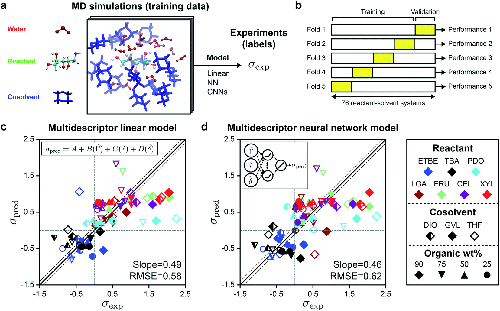 | ||
| Fig. 2 Evaluation of human-selected multidescriptor models. (a) General approach for correlating features from molecular dynamics (MD) simulations to experimental kinetic solvent parameters (σexp). The simulation configuration shows xylitol (XYL) in 90 wt% dioxane (DIO) as an example. (b) Schematic illustrating 5-fold cross validation procedure used to train and validate models. (c) Parity plot between predicted (σpred) and experimental (σexp) kinetic solvent parameters for the multidescriptor linear model. The best-fit slope and root-mean-squared error (RMSE) between σpred and σexp values are shown within the plot. The solid black lines indicate perfect correlation (σpred = σexp), the dashed black lines indicate approximate experimental error, and the dashed gray lines are drawn at σexp = 0 and σpred = 0 as a guide to the eye. (d) Parity plot for the nonlinear fully connected neural network model. | ||
Descriptor values were used as input data to train a linear regression model (eqn (2)) to predict values of the kinetic solvent parameter (σpred):
σpred = A + B(![[capital Gamma, Greek, tilde]](https://www.rsc.org/images/entities/i_char_e1eb.gif) ) + C( ) + C(![[small tau, Greek, tilde]](https://www.rsc.org/images/entities/i_char_e0e5.gif) ) + D( ) + D(![[small delta, Greek, tilde]](https://www.rsc.org/images/entities/i_char_e125.gif) ) ) | (2) |
Fig. 2c shows the parity plot between σpred and σexp for the linear regression model, with each value of σpred corresponding to a validation set prediction from the 5-fold cross validation procedure. We use the best-fit slope and root-mean-square error (RMSE) between σpred and σexp to evaluate model accuracy; a perfect model would have a slope of one and an RMSE of zero. Since the RMSE of the experimental data is 0.10,4 any predictive model with RMSE near 0.10 is sufficiently accurate. The linear model has a slope of 0.49 and an RMSE of 0.58; most outliers are reactions occurring in THF–water (hollow symbols) or in 90 wt% cosolvent systems (diamond symbols). Fitting the linear model using only data for DIO–water mixtures without 5-fold cross validation leads to an RMSE of 0.23,4 but this approach is less accurate for GVL–water (RMSE of 0.36) and THF–water (RMSE of 0.59) mixtures (ESI, Table S3†), indicating that the performance of the linear model depends strongly on the cosolvent. This result suggests that the linear model has limited generalizability across cosolvents. We also tested if a nonlinear model could improve upon the predictions of the linear model using the same input data. We performed 5-fold cross-validation to evaluate a fully connected neural network with three hidden layers, each with ten rectified linear units (ReLU), followed by a linear unit for the regression task of predicting σ using the three human-selected descriptors as input. Fig. 2d shows the parity plot between σpred and σexp using the fully connected neural network model. The behavior of the fully connected neural network model was comparable to that of the linear model with a slope of 0.46 and an RMSE of 0.62. We use these multidescriptor models as a baseline for comparison to alternative models.
These findings show that reaction rates predicted with the multidescriptor models lie in the correct quadrants with few false-positive or false-negative σ values and are accurate for some cosolvents (i.e., DIO). The descriptors underscore the importance of spatial information: Γ quantifies the solvent composition in a region near the reactant, τ describes the relative locations of reactant hydroxyl groups and water molecules, and δ is related to the relative surface areas of hydrophilic and hydrophobic regions of the reactant. However, both models have significant outliers for systems corresponding to larger values of σexp, suggesting that the descriptors fail to capture important information that may be encoded within the complex geometrical (3D) features of the reactant–solvent environment. In addition, the identification of these descriptors requires domain expertise and is time-consuming.
Generation of input data set for interpretation by 3D CNNs using classical MD data
To improve upon the human-selected multidescriptor models, we hypothesized that 3D CNNs can be used to establish mappings between atomic positions sampled from classical MD (which emerge from the combination of reactant–solvent, solvent–cosolvent, and reactant–cosolvent interactions) to experimental reaction rates. We expect that 3D CNNs are appropriate for analyzing these systems because: (i) CNNs can extract non-intuitive features of the reactant–solvent environment by identifying spatial correlations in the input data, (ii) liquid-phase systems exhibit pronounced spatial correlations due to intermolecular interactions between solvent molecules, (iii) the importance of spatial information encoded within the human-selected descriptors suggests that spatial correlations are relevant to solvent effects, and (iv) 3D CNNs can analyze atomic positions without transforming the domain to a 2D space (flattening), thereby capturing the detailed geometry of the reactant and local solvation environment. 3D CNNs thus provide a natural framework for identifying complex features of reactant–solvent environments that affect reaction rates but that may not be easily identified using human intuition.We first developed a protocol for converting trajectory data of atomic positions of reactant, solvent, and cosolvent molecules obtained from classical MD simulations into a data representation that is suitable for 3D CNN analysis. 3D CNNs interpret data consisting of a series of voxels arranged in a 3D grid, with each voxel containing normalized intensities in several independent channels. The channels can convey different types of field information. The relative positioning of the voxels in the grid confers spatial information. We thus converted the spatially continuous atomic positions output by MD to voxels that record the normalized occurrences of water, cosolvent, and reactant oxygen atoms within (0.2 nm)3 volume elements. This data representation is motivated by the physical intuition obtained from the success of the human-selected multidescriptor models: the importance of the descriptor Γ suggests that the positions of water and cosolvent atoms should be recorded to quantify preferential enrichment of solvent molecules near the reactant while the descriptors τ and δ suggest that the positions of reactant oxygen atoms should be recorded to quantify potential hydrogen bonding and reactant hydrophilicity. The volume associated with each voxel was selected to be comparable to typical atomic radii to ensure that molecular geometry could be resolved.
Fig. 3 illustrates the approach used to convert MD positions to a grid of voxels. For each set of atomic positions corresponding to a single time sampled during a MD trajectory (i.e., a MD configuration), we centered a 3D histogram on the center-of-mass of the reactant. The histogram covered a cubic (4 nm)3 volume (a volume smaller than the total simulation box size to avoid crossing the simulation box boundaries) that was divided into a 20 × 20 × 20 grid of bins corresponding to (0.2 nm)3 volume elements. For each bin, we calculated the normalized occurrence of water atoms by counting the number of water atoms within the bin and normalizing by the maximum number of water atoms within any bin. The same procedure was separately performed to calculate the normalized occurrence of cosolvent and reactant oxygen atoms in each bin. The normalized water, reactant, and cosolvent occurrences were then stored in the “red, green, and blue” color channels, respectively (Fig. 3a) to obtain a 20 × 20 × 20 × 3 grid of voxels for a single MD configuration.
 | ||
| Fig. 3 Input data representation for 3D CNNs. Approach for converting the atomic positions obtained from a MD simulation to a voxel representation using xylitol in 90 wt% dioxane as an example. (a) For each MD configuration (example at left), a (4 nm)3 cubic box was centered on the reactant and a 20 × 20 × 20 grid of (0.2 nm)3 volume elements was used to discretize space. The normalized occurrences of water, oxygens of the reactant, and cosolvent atomic positions within each volume element were stored in different channels to yield a 20 × 20 × 20 × 3 grid of voxels. Voxels are visualized by showing the water channel in red, the reactant channel in green, and the cosolvent channel in blue. Half of the voxels are transparent to illustrate the solvent distribution around the reactant. (b) Grids of voxels were averaged over 2 ns of MD data (200 MD configurations) to yield a 20 × 20 × 20 × 3 voxel representation. (c) For each reactant–solvent system, 20 ns of simulation data were used to generate 10 independent voxel representations. | ||
To capture the preferential locations of solvent molecules relative to the reactant as they diffuse within the cubic volume, and to prevent voxels from being unoccupied, we averaged grid values obtained from multiple consecutive MD configurations to generate a single averaged grid of voxels that we define as a voxel representation. Specifically, each voxel representation was generated by averaging grid values from 2 ns of MD data (corresponding to 200 consecutive MD configurations) as illustrated in Fig. 3b. The 2 ns simulation time was selected as a balance between maximizing model accuracy and minimizing computational expense. This simulation time is substantially shorter than the 205 ns trajectories associated with each training label. Thus, we split the first 20 ns of each trajectory into 10 independent 2 ns partitions and generated a voxel representation for each partition, yielding 10 voxel representations per training label. These choices were based on extensive robustness tests to determine the best-performing input data representations as described in the ESI, Section S5 (Table S4).† Because 3D CNNs are not rotationally invariant, we further augmented the training data by rotating each voxel representation to generate 24 unique cube rotations per voxel representation (Fig. S1†), leading to 240 (augmented) voxel representations per training set label.
3D CNNs improve reaction rate predictions with less required simulation time
We next developed a 3D CNN model, which we call SolventNet, that inputs voxel representations and outputs predicted kinetic solvent parameters. The SolventNet architecture consists of four convolutional layers, two max-pooling layers, and three fully connected layers as shown schematically in Fig. 4a. This architecture is based on the previously developed VoxNet 3D CNN but replaces the final fully connected layer with two convolutional layers, one max-pooling layer, and three fully connected layers.31 We also compared SolventNet to the VoxNet31 and ORION30 3D CNNs (ESI, Fig. S4†) to investigate how the 3D CNN architecture influences prediction accuracy. All three models include a final layer with a linear activation unit for the regression task of predicting σ.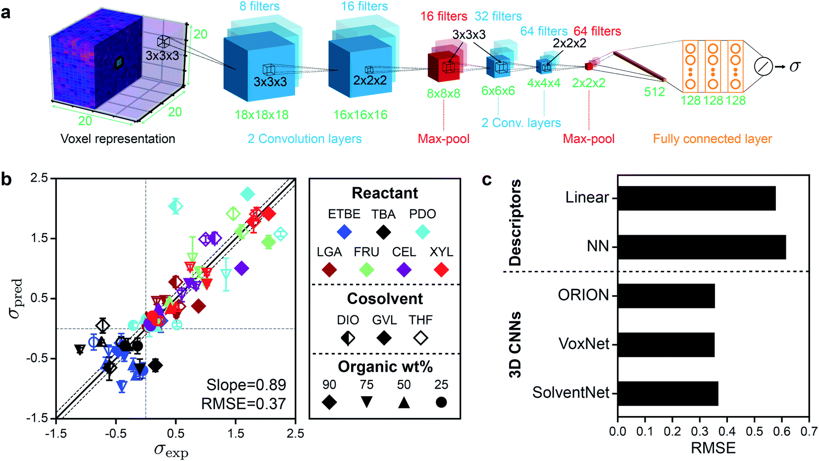 | ||
| Fig. 4 Architecture, training, and performance of 3D CNNs. (a) Architecture of SolventNet, a 3D CNN that inputs a 20 × 20 × 20 × 3 voxel representation (described in Fig. 3) and outputs the predicted kinetic solvent parameter (σ). 3D CNNs were evaluated using the same 5-fold cross validation procedure described in Fig. 2b. (b) Parity plot between predicted (σpred) and experimental (σexp) kinetic solvent parameters using SolventNet. σpred is the average prediction of 10 voxel representations per label. Error bars show the standard deviation of these predictions. The best-fit slope and root-mean-squared error (RMSE) between σpred and σexp values are shown within the plot. Solid and dashed lines follow the conventions of Fig. 2. (c) Comparison of the RMSEs between σpred and σexp for the multidescriptor linear and nonlinear neural network (NN) models and the 3D CNNs (ORION, VoxNet, and SolventNet) when performing 5-fold cross validation. | ||
The 3D CNNs were evaluated using 5-fold cross-validation, similar to the procedure used for the human-selected descriptor models. For the 3D CNNs, the training data included all augmented voxel representations for 80% of the labels (14400 or 14640 voxel representations) and the validation data included only non-augmented voxel representations for the remaining 20% of the labels (150 or 160 voxel representations). Fig. 4b shows the parity plot between σpred and σexp using SolventNet. Values and error bars of σpred report the average and standard deviation of the values predicted for each of the 10 non-augmented validation set voxel representations per label. Compared to the baseline human-selected multidescriptor models (Fig. 2), SolventNet significantly improves the prediction of kinetic solvent parameters with a best-fit slope of 0.89 and an RMSE of 0.37. Fig. 4c further indicates that the RMSEs obtained using all three 3D CNNs (SolventNet, VoxNet, and ORION) are comparable and outperform the multidescriptor models. Moreover, the 3D CNNs were trained using only 20 ns of MD data per reactant–solvent combination compared to the 205 ns of MD data per reactant–solvent combination used to compute the three descriptors in eqn (2). The 3D CNNs required 1.6–2.4 hours to train using one GPU and one CPU core (Table S3†), whereas the MD simulations required ∼216 hours for all 76 reactant–solvent combinations using one GPU and 28 CPU cores, a substantially longer time. Therefore, the ∼10-fold reduction in MD data translates to a comparable decrease in real time required for model training.
A potential issue when training CNNs is the large number of learned parameters, which may lead to overfitting. We note, however, that the 3D CNNs used in this work are relatively compact; SolventNet has 172417 parameters compared to 33601345 parameters for VGG16, a common 2D CNN35 (Methods and Table S3†). The ratio of parameters to the number of augmented training voxel representations for SolventNet is 11.8–11.9; for comparison, the ratio of parameters to the number of training descriptor sets for the fully connected neural network model is 4.4. The small ratio of parameters to training examples for SolventNet is comparable to alternative 3D CNN architectures and suggests that we should not expect significant overfitting during training. For example, 3D CNNs have been used to assess the quality of protein tertiary structures with a ratio of parameters to training examples of 34 (∼5.4 million parameters, ∼160000 grids of voxels)36 and 85 (∼170 million parameters, ∼2 million grids of voxels).37 We also observe that increasing the amount of training voxel representations by a factor of 10 (by splitting 200 ns of MD data into 100 voxel representations) does not impact 3D CNN performance (Fig. S3†). Moreover, the differences in RMSE between ORION, VoxNet, and SolventNet show that CNN architecture minimally affects model performance, even though ORION has nearly five times as many parameters as SolventNet. Therefore, the specific 3D CNN architecture is not critical; rather, it is the use of a 3D CNN to analyze MD simulations that yield improved model performance. We also tested alternative neural network architectures (ESI†), including networks with both descriptors and voxel representations as input, 2D CNNs, and 3D CNNs with alternative voxel representations, but did not observe increases in accuracy. Together, these results show that 3D CNNs are more accurate than prior models based on human-selected descriptors (Fig. 2) while requiring less MD data to train, that the amount of training data used is sufficient, and that prediction accuracy does not significantly vary with model architecture. For the remainder of the manuscript, we focus on SolventNet because it has the median number of parameters and performs well when predicting the test set as discussed in the next section (see Table S3† for model comparisons).
Generalizability of SolventNet predictions to new solvents and reactants
We next assessed the accuracy of SolventNet for the 32 reactant–solvent combinations included in the test set. For each test set reactant–solvent combination, we performed new MD simulations to obtain the 4 ns of simulation data necessary to generate two voxel representations (following the same procedure illustrated in Fig. 3). Only two voxel representations were used to assess the ability of SolventNet to rapidly generalize to new solvent combinations with minimal MD simulation data. The test set voxel representations were not augmented. We re-trained SolventNet using all training set data (76 labels and 18240 augmented voxel representations) and then predicted kinetic solvent parameters for the test set voxel representations.
Fig. 5 shows the parity plot between σpred and σexp for the test set using SolventNet. Values and error bars of σpred report the average and standard deviation of the values predicted for each of the 2 test set voxel representations per label. The best-fit slope is 0.72 and the RMSE is 0.48, indicating that while prediction accuracy slightly degrades compared to predictions for the validation set, SolventNet still generalizes well. Notably, the test set accuracy exceeds the validation set accuracy of the baseline multidescriptor models. The parity plot also shows high linear correlation with Pearson's r = 0.80 for the test set data. Thus, even for systems for which SolventNet predictions are less accurate, the model still captures qualitative trends regarding solvent compositions that improve reaction rates, despite including reactants (GLU), cosolvents (MeCN, DMSO, and ACE), and organic weight fractions (44, 65, and 88 wt%) not present for any of the reactant–solvent combinations in the training set. These findings suggest that SolventNet extracted features of the reactant–solvent environment that are important to reaction performance and that are generalizable across different reactant–solvent combinations. The reduced accuracy may be due, in part, to the different literature sources for the test set data (which may introduce experimental error) and the use of a hydrochloric acid rather than triflic acid catalyst in ref. 33, since chloride can impact reaction kinetics.6
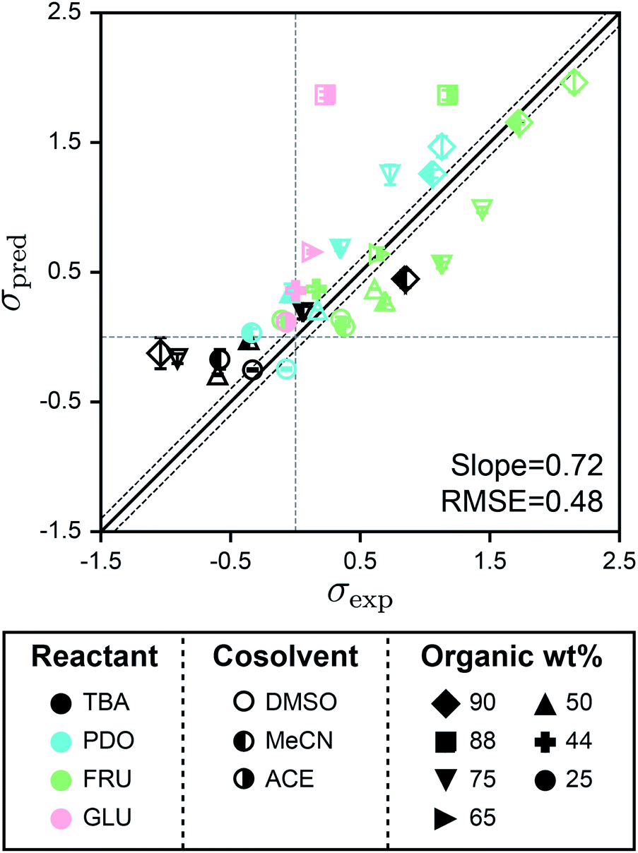 | ||
| Fig. 5 Generalizability of SolventNet to new reactants and cosolvents. Parity plots between predicted (σpred) and experimental (σexp) kinetic solvent parameters for the test set. Predictions were made using SolventNet after training with all training set data. σpred is the average prediction of 2 voxel representations per label. Error bars show the standard deviation of these predictions. The slope and root-mean-squared error (RMSE) between σpred and σexp values are shown within each plot. Solid and dashed lines follow the convention of Fig. 2. | ||
The test set results show that SolventNet performs well for DMSO–water mixtures with an RMSE of 0.43. This result is somewhat surprising because DMSO is more basic than the cosolvents used for training3 and is known to compete against water for binding sites around hydroxyl groups on hydrophilic reactants.12,14 In addition, we have previously found that reactant–DMSO interactions can be favored over reactant–water interactions in DMSO–water mixtures, whereas reactant–water interactions are favored in the other cosolvent–water systems.15 Despite these unique behaviors, the features learned by SolventNet can translate to reaction rate predictions for DMSO–water mixtures with accuracy comparable to predictions for all other systems tested. Of the reactants in the test set, the worst prediction accuracy was obtained for GLU with an RMSE of 0.88. Since GLU was not part of the training set, we expect that the prediction accuracy for this reactant would be lower than FRU; moreover, this system used a hydrochloric acid catalyst as noted above. Nonetheless, the qualitative trend is again captured for GLU conversion with a Pearson's r = 0.93 (computed only for systems with GLU).
Based on the DMSO and GLU analysis, we also used leave-one-out cross-validation to determine if SolventNet predictions were sensitive to particular reactants or cosolvents included in the training set, further motivated by the weak performance of descriptor-based models for THF– and GVL–water mixtures. In this procedure (illustrated in Fig. 6a), we held out all labels and associated voxel representations for reactant–solvent combinations in the original training set that either contained a given cosolvent (e.g., all DIO–water mixtures) or a given reactant (e.g., XYL in all solvent systems) and used these data as the test set. SolventNet was trained using the remaining data and used to predict kinetic solvent parameters for 10 voxel representations per test set reactant–solvent combination. This procedure was repeated by iteratively using data for each cosolvent or reactant as the test set. Fig. 6b shows the parity plot between σpred and σexp for leave-one-out cross validation across cosolvents. The RMSE varies between 0.27–0.43, which is comparable to the predictions for DMSO–water mixtures. These results indicate that SolventNet predictions are comparable for a wide range of mixed-solvent environments, including the THF– and GVL–water mixtures that were poorly predicted by the linear multidescriptor model. Fig. 6c shows the parity plot between σpred and σexp for leave-one-out cross validation across reactants. The RMSE varies between 0.11–0.81 depending on the specific reactant, which is comparable to the results for leave-one-out cross validation across cosolvents. The largest RMSE is obtained for LGA which is comparable to the test set results for GLU. As with the GLU results, σpred and σexp for LGA exhibit strong linear correlation with a r of 0.90, indicating that quantitative trends of reactivity are captured. LGA may be an outlier due to the overestimation of its hydrophilicity since the voxel representations account for all oxygens of LGA, including oxygens in ether bonds. Taken together, the results from the independent test set and from leave-one-out cross-validation suggest that SolventNet predictions generalize well across all cosolvents tested and all reactants other than LGA.
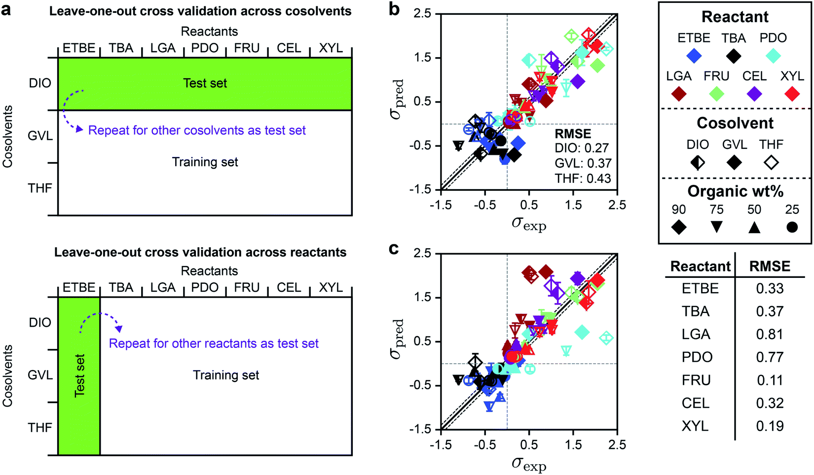 | ||
| Fig. 6 Leave-one-out cross validation of SolventNet. (a) Schematic illustrating the leave-one-out cross validation procedure in which all data for a single cosolvent or all data for a single reactant were used as the test set and the remaining data were used as the training set. (b) Parity plot between predicted (σpred) and experimental (σexp) kinetic solvent parameters for the leave-one-out cross validation of SolventNet across cosolvents. The RMSE values between σpred and σexp labeled within each plot report the values obtained when data for the listed cosolvent–water system were used to as the test set. σpred is the average prediction of 10 voxel representations per label. Error bars show the standard deviation of these predictions. Solid and dashed lines follow the conventions of Fig. 2. (c) Parity plot between predicted (σpred) and experimental (σexp) kinetic solvent parameters for the leave-one-out cross validation of SolventNet across reactants. The RMSE values in the table report the values obtained when data for the listed reactant were used as the test set. | ||
Physical interpretation of SolventNet features
While SolventNet offers improved prediction accuracy and computational efficiency compared to models based on human-selected descriptors, it is difficult to physically interpret features extracted by the model.38 For example, representative voxel representations for different reactant–solvent combinations do not have visually distinctive features (Fig. S2†). As an initial step toward interpreting features recognized by SolventNet, we generated saliency maps to visualize the sensitivity of SolventNet predictions to different voxels and thus to specific spatial regions around the reactant. A saliency map consists of saliency values (normalized between 0–1) for each voxel that indicate how sensitive the SolventNet prediction is to the normalized occurrences of water, reactant, and cosolvent atoms in that voxel. Larger saliency values indicate increased sensitivity. Fig. 7 shows a saliency map that was generated using the integrated gradient approach39 (described in the Methods) by inputting a voxel representation of XYL in 90 wt% DIO to a fully trained SolventNet model. The saliency map is split into separate 3D grids of voxels for reactant, cosolvent, and water channels, with each voxel colored according to its normalized saliency value using the same color scheme as the input voxel representation (Fig. 3). Transparent voxels are unimportant to model predictions (normalized saliency values less than 0.10).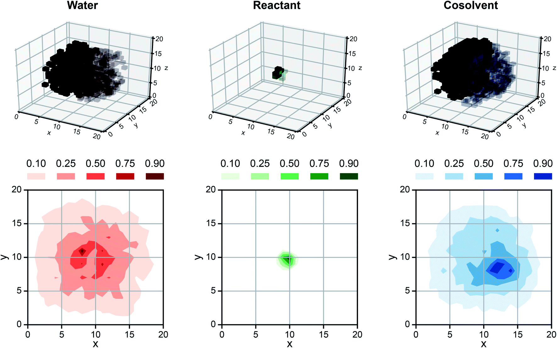 | ||
| Fig. 7 Saliency map using SolventNet. Example saliency map generated for a voxel representation of XYL in 90 wt% DIO (shown in Fig. 4a) using SolventNet after training with all training set data. The saliency map is visualized on a 3D grid with the same dimensions as the input voxel representation. Each voxel is assigned a saliency value normalized from 0 to 1 that indicates the sensitivity of SolventNet predictions to the normalized occurrences of water, reactant, and cosolvent atoms in that voxel. Larger saliency values indicate greater sensitivity. The saliency map is visualized by separate grids showing the water value in red, the reactant value in green, and the cosolvent value in blue. Half of the voxels are transparent to illustrate the saliency values around the reactant and only the voxels with values greater than 0.10 for each system component are shown. 2D contours are plotted by averaging along the z-axis for normalized values of 0.10, 0.25, 0.50, 0.75, and 0.90. | ||
Inspection of the saliency map in Fig. 7 confirms that SolventNet primarily recognizes features of the solvent environment within a local domain near the reactant, in agreement with the assumption underlying the definition of human-selected descriptors. Saliency maps for each channel are further projected from 3D to 2D by averaging saliency values along the z-axis (selected arbitrarily) to generate the contour plots shown in Fig. 7. These plots clearly show that regions near the reactant are most important for predictions, that the size of the simulated volume is sufficiently large that regions far from the reactant are unimportant, and that SolventNet extracts non-intuitive geometrical features that are not captured by the assumptions of spherical symmetry. Similar saliency maps may be useful for guiding future ab initio calculations by identifying important solvent regions to be studied, thus minimizing the number of molecules needed for quantum chemical calculations.
Conclusions
In this work, we combined machine learning tools with classical MD simulations to develop SolventNet, a 3D CNN which interprets MD simulation data that has been transformed into a voxel representation to predict acid-catalyzed reaction rates in aqueous mixtures with polar aprotic cosolvents. SolventNet does not require the human selection of descriptors a priori and can capture spatial correlations without assuming spherical symmetry. SolventNet (and other 3D CNNs) more accurately predicts reaction rates than models based on human-selected descriptors and generalizes to new polar aprotic cosolvents, cosolvent mass fractions, and reactants not used during model training. These findings indicate that SolventNet extracts features from the spatial configurations of reactant, solvent, and cosolvent molecules determined by classical MD simulations that encode sufficient information to predict solvent effects on acid-catalyzed reactions, even though the reaction mechanisms and possible transition states are not explicitly modeled.A significant advantage of this newly developed approach is computational efficiency. Once trained, SolventNet requires as little as 4 ns of MD simulation data to predict a reaction rate for a single reactant–solvent combination. For the system sizes considered in this work, these trajectories can be simulated in less than an hour on single node of a typical high-performance computing cluster, greatly diminishing the time necessary to predict reaction rates compared to ab initio methods. This reduced computational expense suggests that SolventNet could be leveraged for solvent screening, potentially in combination with process models,10 to design more efficient biomass conversion processes without costly experimental trial-and-error. However, all systems studied so far involve mixtures of water and polar aprotic cosolvents; extending SolventNet to predict reaction rates in substantially different solvent systems (e.g., ionic liquids) will likely require additional training.
The voxel representations input to SolventNet also only contain atomic positions, thus omitting important chemical information such as the presence of covalent bonds between atoms and atomic charges. These data could possibly be interpreted by alternative network architectures. For example, a graph neural network could represent atoms as nodes and atomic interactions as edges.16,17,40 Thus, we anticipate that further model development can continue to increase prediction accuracy. Furthermore, the voxel representations input to SolventNet are only generated from MD simulations of reactant states; future work will explore whether including voxel representations from simulations of product states can improve the accuracy of reaction rate predictions or enable predictions of reaction selectivities.14 Classical MD can also model molecules much larger than the small-molecule reactants studied here, such as biomass-relevant polymers (e.g., cellulose, hemicellulose, or lignin).11–13 Future work will explore the use of SolventNet with semantic segregation techniques, which enable individual regions of data input to a CNN to be separately classified,41 to predict the reactivity of multiple reactive sites simultaneously based on MD simulations of biomass-relevant polymers. Screening solvents for these larger systems is difficult with ab initio methods.
Methods
Classical molecular dynamics simulation methods
Classical MD simulations were performed using a leapfrog integrator with a 2 fs timestep. The initial simulation box dimensions were set to (6 nm)3 in all simulations, and water and cosolvent molecules were added in the desired proportions. All reactants and cosolvents were parameterized using the CGenFF/CHARMM36 force fields.42–44 Water was modeled using the Single Point Charge/Extended (SPC/E) model.45 Verlet lists were generated using a 1.2 nm neighbor list cutoff. van der Waals interactions were modeled with a Lennard-Jones potential that was smoothly shifted to zero between 1.0 nm and 1.2 nm. Electrostatic interactions were calculated using the smooth particle mesh Ewald method with a short-range cutoff of 1.2 nm, grid spacing of 0.12 nm, and 4th order interpolation. Bonds were constrained using the LINCS algorithm.46 The solvent system was equilibrated in a NPT simulation for 5 ns at T = 300 K and P = 1 bar with a velocity-rescale thermostat and Berendsen barostat. A single reactant molecule was added to the system and equilibrated with the same barostat and thermostat for 500 ps. NPT production simulations were then performed at the reaction temperature and P = 1 bar using a Nose–Hoover thermostat and Parrinello–Rahman barostat. All thermostats used a 1.0 ps time constant and all barostats used a 5.0 ps time constant with an isothermal compressibility of 5.0 × 10⁻⁵ bar−1. Simulation configurations were output every 10 ps. All simulations were performed using GROMACS 201647 and visualized using VMD.48
Simulation data obtained using this protocol for reactant–solvent combinations included in the training set (including molecules drawn in black in Fig. 1c and d) were taken from ref. 4. The production simulations for these molecules were performed for 200 ns. This simulation time was necessary due to the slow convergence of Γ as described in ref. 4. The last 190 ns were used to compute Γ and δ for the multidescriptor models shown in Fig. 2. An additional 5 ns production simulation was performed to compute τ. Descriptors were calculated as described in ref. 4 (values listed in Table S1†). The first 20 ns of the 200 ns were used to generate voxel representations for training and validating the 3D CNNs. New simulations were performed following the above simulation protocol for the reactant–solvent combinations included in the test set (including molecules drawn in gray in Fig. 1c and d). The production simulations for these molecules were performed for 4 ns at the reaction temperatures (listed in Table S2†) and used to generate voxel representations for testing the 3D CNNs.
Summary of model training, validation, and testing
108 experimentally determined reaction rates from literature sources were converted to kinetic solvent parameters using eqn (1) and used as labels. Each reaction rate (label) was determined for a unique reactant–solvent combination, which is defined as a single reactant in a binary mixture of a single cosolvent and water (in varying wt%). The labels were split into a training set with 72 labels (70% of the labels), all from ref. 4, and a test set with 32 labels (30% of the labels) from ref. 3 and 33. A single MD trajectory was associated with each label. All models were evaluated using a 5-fold cross-validation procedure in which 80% of the labels and associated descriptors/voxel representations (60–61 labels) were used as training data and the remaining 20% of the labels (15–16 labels) and associated descriptors/voxel representations were used as validation data. This procedure was iterated 5 times such that each label was used for validation once. Model performance was evaluated based on the RMSE of the predicted values of the kinetic solvent parameter for the validation set.Training data for the multidescriptor models were generated by using each MD trajectory to compute 3 descriptors from 205 ns of MD data as described above. The multidescriptor linear model was trained by regressing a line to the training data. The multidescriptor fully connected neural network was trained for 500 epochs (for each epoch, the neural network trained one cycle of the entire dataset) using the Keras deep learning library on top of Tensorflow.49 Training was performed using the Adam optimizer with a learning rate of 0.001, mean-squared loss function, and training batches of size 18 (one epoch equates to four backpropagation steps).
Training data for the 3D CNNs were generated by splitting each MD trajectory associated with a training set label into 10 independent partitions containing 2 ns (200 MD configurations) of consecutive MD data. For each partition, all MD configurations were converted to 3D grids of voxels that were averaged to obtain voxel representations as described in the Results and discussion (Fig. 3). The 10 voxel representations per label used for training were augmented by including all 24 unique cube rotations as training data, leading to a total of 240 voxel representations per label or 14400–14640 training voxel representations. The voxel representations per label used for validation were not augmented, leading to 150–160 validation voxel representations. All 3D CNNs were trained for 500 epochs using the Keras deep learning library on top of Tensorflow.49 Models were trained using the Adam optimizer with a learning rate of 0.00001, mean-squared loss function, and training batches of size 18 (one epoch equates to 814 backpropagation steps). Learning curves for all 3D CNNs are shown in Fig. S5 of the ESI.†
The generalizability of SolventNet was assessed using the test set and leave-one-out cross-validation of the training set. For each test set label, 4 ns of consecutive MD data was converted to two independent voxel representations that were not augmented. SolventNet was re-trained using augmented voxel representations for all training set data (18240 voxel representations) and used to predict kinetic solvent parameters for the 2 voxel representations per test set label (64 voxel representations). In the leave-one-out cross-validation procedure, all labels associated with a single reactant or cosolvent in the training set were held out as the test set, then SolventNet was trained using all data for the remaining labels and used to predict kinetic solvent parameters for 10 voxel representations per held out label. In both procedures, model performance was assessed based on the RMSE of the predicted values of the kinetic solvent parameter for the test set.
3D CNN architectures
Three 3D CNN architectures that vary in complexity and number of parameters were considered in this work: VoxNet31 (5 layers, 150689 parameters), ORION30 (8 layers, 908833 parameters), and SolventNet (9 layers, 172417 parameters), which we developed in-house. The architectures of VoxNet and ORION are described in the ESI (Fig. S4).† SolventNet has three stages (Fig. 4a). The first stage has two convolutional layers with 8 and 16 3 × 3 × 3 filters, respectively, and a 2 × 2 × 2 max-pooling layer. The second stage has the same structure as the first, except the two convolutional layers have 32 and 64 filters, respectively. The results from the last max-pooling layer are passed to a batch normalization layer and flattened. The flattened data is then input to a neural network with three fully connected layers with 128 nodes in each layer. The ReLU activation function is used for the fully connected layers.
Generation of saliency maps
Saliency maps were computed using a fully trained SolventNet with the integrated gradient approach.39 We define the voxel representation input as a tensor . SolventNet has a loss function
  , where the output is the RMSE loss value. Eqn (3) defines the saliency map function
  :
: | (3) |
![[x with combining macron]](https://www.rsc.org/images/entities/i_char_0078_0304.gif) is the baseline input, which we select as = 0. Eqn (3) accounts for the change of the loss function caused by the change in the normalized occurrences of atoms in a voxel in the original input voxel representation. If the loss function does not significantly change, then that voxel is considered to be unimportant for the prediction. Values of E(x), normalized to lie within the range 0–1, are shown on the saliency maps in Fig. 7.
is the baseline input, which we select as = 0. Eqn (3) accounts for the change of the loss function caused by the change in the normalized occurrences of atoms in a voxel in the original input voxel representation. If the loss function does not significantly change, then that voxel is considered to be unimportant for the prediction. Values of E(x), normalized to lie within the range 0–1, are shown on the saliency maps in Fig. 7.
Author contributions
AKC and RCV designed, performed, and analyzed the molecular dynamics simulations and the voxel representations used for SolventNet. SJ, WZ, and VMZ developed SolventNet and other 3D CNN architectures used to analyse voxel representations. All authors interpreted the results and wrote the manuscript.Conflicts of interest
There are no competing interests.Acknowledgements
This work was supported in part by the Great Lakes Bioenergy Research Center, U.S. Department of Energy, Office of Science, Office of Biological and Environmental Research under Award Numbers DE-SC0018409. This work used the Extreme Science and Engineering Discovery Environment (XSEDE), which is supported by National Science Foundation grant number ACI-1549562. This work also used the computing resources and assistance of the UW-Madison Center for High Throughput Computing (CHTC) in the Department of Computer Sciences. The CHTC is supported by UW-Madison, the Advanced Computing Initiative, the Wisconsin Alumni Research Foundation, the Wisconsin Institutes for Discovery, and the National Science Foundation, and is an active member of the Open Science Grid, which is supported by the National Science Foundation and the U.S. Department of Energy's Office of Science. The authors acknowledge support from the Department of Chemical and Biological Engineering at the University of Wisconsin-Madison and the Wisconsin Alumni Research Fund. Finally, the authors gratefully acknowledge partial support of this research by NSF through the University of Wisconsin Materials Research Science and Engineering Center (DMR-1720415).References
- L. Shuai and J. Luterbacher, ChemSusChem, 2016, 9, 133–155 CrossRef CAS.
- M. A. Mellmer, C. Sener, J. M. R. Gallo, J. S. Luterbacher, D. M. Alonso and J. A. Dumesic, Angew. Chem., Int. Ed., 2014, 53, 11872–11875 CrossRef CAS.
- M. A. Mellmer, C. Sanpitakseree, B. Demir, P. Bai, K. W. Ma, M. Neurock and J. A. Dumesic, Nat. Catal., 2018, 1, 199–207 CrossRef CAS.
- T. W. Walker, A. K. Chew, H. X. Li, B. Demir, Z. C. Zhang, G. W. Huber, R. C. Van Lehn and J. A. Dumesic, Energy Environ. Sci., 2018, 11, 617–628 RSC.
- J. J. Varghese and S. H. Mushrif, React. Chem. Eng., 2019, 4, 165–206 RSC.
- M. A. Mellmer, C. Sanpitakseree, B. Demir, K. Ma, W. A. Elliott, P. Bai, R. L. Johnson, T. W. Walker, B. H. Shanks, R. M. Rioux, M. Neurock and J. A. Dumesic, Nat. Commun., 2019, 10, 1132 CrossRef.
- S. H. Mushrif, J. J. Varghese and C. B. Krishnamurthy, Phys. Chem. Chem. Phys., 2015, 17, 4961–4969 RSC.
- S. Caratzoulas and D. G. Vlachos, Carbohydr. Res., 2011, 346, 664–672 CrossRef CAS.
- G. Tsilomelekis, T. R. Josephson, V. Nikolakis and S. Caratzoulas, ChemSusChem, 2014, 7, 117–126 CrossRef CAS.
- J. He, M. Liu, K. Huang, T. W. Walker, C. T. Maravelias, J. A. Dumesic and G. W. Huber, Green Chem., 2017, 19, 3642–3653 RSC.
- A. S. Patri, B. Mostofian, Y. Pu, N. Ciaffone, M. Soliman, M. D. Smith, R. Kumar, X. Cheng, C. E. Wyman, L. Tetard, A. J. Ragauskas, J. C. Smith, L. Petridis and C. M. Cai, J. Am. Chem. Soc., 2019, 141(32), 12545–12557 CrossRef CAS.
- S. H. Mushrif, S. Caratzoulas and D. G. Vlachos, Phys. Chem. Chem. Phys., 2012, 14, 2637–2644 RSC.
- J. V. Vermaas, L. Petridis, J. Ralph, M. F. Crowley and G. T. Beckham, Green Chem., 2019, 21, 109–122 RSC.
- A. K. Chew, T. W. Walker, Z. Shen, B. Demir, L. Witteman, J. Euclide, G. W. Huber, J. A. Dumesic and R. C. Van Lehn, ACS Catal., 2020, 10, 1679–1691 CrossRef CAS.
- A. K. Chew and R. C. Van Lehn, Front. Chem., 2019, 7, 439 CrossRef CAS.
- C. W. Coley, W. Jin, L. Rogers, T. F. Jamison, T. S. Jaakkola, W. H. Green, R. Barzilay and K. F. Jensen, Chem. Sci., 2019, 10, 370–377 RSC.
- D. K. Duvenaud, D. Maclaurin, J. Iparraguirre, R. Bombarell, T. Hirzel, A. Aspuru-Guzik and R. P. Adams, Convolutional Networks on Graphs for Learning Molecular Fingerprints, Advances in neural information processing systems, 2015, pp. 2224–2232 Search PubMed.
- R. Gómez-Bombarelli, J. N. Wei, D. Duvenaud, J. M. Hernández-Lobato, B. Sánchez-Lengeling, D. Sheberla, J. Aguilera-Iparraguirre, T. D. Hirzel, R. P. Adams and A. Aspuru-Guzik, ACS Cent. Sci., 2018, 4, 268–276 CrossRef.
- N. E. Jackson, A. S. Bowen, L. W. Antony, M. A. Webb, V. Vishwanath and J. J. de Pablo, Sci. Adv., 2019, 5, eaav1190 CrossRef CAS.
- E. Y. Lee, B. M. Fulan, G. C. L. Wong and A. L. Ferguson, Proc. Natl. Acad. Sci. U. S. A., 2016, 113, 13588–13593 CrossRef CAS.
- Z. Wu, B. Ramsundar, E. N. Feinberg, J. Gomes, C. Geniesse, A. S. Pappu, K. Leswing and V. Pande, Chem. Sci., 2018, 9, 513–530 RSC.
- S. Chmiela, A. Tkatchenko, H. E. Sauceda, I. Poltavsky, K. T. Schütt and K.-R. Müller, Sci. Adv., 2017, 3, e1603015 CrossRef.
- W. Rawat and Z. H. Wang, Neural Comput., 2017, 29, 2352–2449 CrossRef.
- A. Krizhevsky, I. Sutskever and G. E. Hinton, presented in part at the Proceedings of the 25th International Conference on Neural Information Processing Systems, Lake Tahoe, Nevada, 2012, vol. 1 Search PubMed.
- O. Russakovsky, J. Deng, H. Su, J. Krause, S. Satheesh, S. Ma, Z. H. Huang, A. Karpathy, A. Khosla, M. Bernstein, A. C. Berg and L. Fei-Fei, Int. J. Comput. Vis., 2015, 115, 211–252 CrossRef.
- R. D. Singh, A. Mittal and R. K. Bhatia, Multimed. Tool. Appl., 2019, 78, 15951–15995 CrossRef.
- W. Torng and R. B. Altman, Bioinformatics, 2018, 35, 1503–1512 CrossRef.
- J. Jiménez, S. Doerr, G. Martínez-Rosell, A. S. Rose and G. De Fabritiis, Bioinformatics, 2017, 33, 3036–3042 CrossRef.
- J. Jiménez, M. Škalič, G. Martínez-Rosell and G. De Fabritiis, J. Chem. Inf. Model., 2018, 58, 287–296 CrossRef.
- N. Sedaghat, M. Zolfaghari, E. Amiri and T. Brox, 2016, arXiv preprint arXiv:1604.03351.
- D. Maturana and S. Scherer, 2015 IEEE/RSJ International Conference on Intelligent Robots and Systems (IROS), 2015, pp. 922–928 Search PubMed.
- D. M. Alonso, S. H. Hakim, S. Zhou, W. Won, O. Hosseinaei, J. Tao, V. Garcia-Negron, A. H. Motagamwala, M. A. Mellmer, K. Huang, C. J. Houtman, N. Labbé, D. P. Harper, C. T. Maravelias, T. Runge and J. A. Dumesic, Sci. Adv., 2017, 3, e1603301 CrossRef.
- A. H. Motagamwala, K. Huang, C. T. Maravelias and J. A. Dumesic, Energy Environ. Sci., 2019, 12(7), 2212–2222 RSC.
- S. Raschka, 2018, arXiv preprint arXiv:1811.12808.
- K. Simonyan and A. Zisserman, 2014, arXiv preprint arXiv:1409.1556.
- G. Derevyanko, S. Grudinin, Y. Bengio and G. Lamoureux, Bioinformatics, 2018, 34, 4046–4053 CrossRef CAS.
- R. Sato and T. Ishida, PLoS One, 2019, 14(9), e0221347 CrossRef CAS.
- J. Yosinski, J. Clune, A. Nguyen, T. Fuchs and H. Lipson, 2015, arXiv preprint arXiv:1506.06579.
- M. Sundararajan, A. Taly and Q. Yan, Proceedings of the 34th International Conference on Machine Learning, 2017, vol. 70, pp. 3319–3328 Search PubMed.
- Z. Ying, J. You, C. Morris, X. Ren, W. Hamilton and J. Leskovec, Adv. Neural Inf. Process. Syst., 2018, 4800–4810 Search PubMed.
- Y. Guo, Y. Liu, T. Georgiou and M. S. Lew, Int. J. Multimed. Inf. Retr., 2018, 7, 87–93 CrossRef.
- R. B. Best, X. Zhu, J. Shim, P. E. M. Lopes, J. Mittal, M. Feig and A. D. MacKernell Jr, J. Chem. Theory Comput., 2013, 8, 3257–3273 CrossRef.
- K. Vanommeslaeghe, E. Hatcher, C. Acharya, S. Kundu, S. Zhong, J. Shim, E. Darian, O. Guvench, P. Lopes, I. Vorobyov and A. D. MacKernell Jr, J. Comput. Chem., 2009, 31, 671–690 Search PubMed.
- W. Yu, X. He, K. Vanommeslaeghe and A. D. MacKernell Jr, J. Comput. Chem., 2012, 33, 2451–2468 CrossRef CAS.
- H. J. C. Berendsen, J. R. Grigera and T. P. Straatsma, J. Phys. Chem., 1987, 91, 6269–6271 CrossRef CAS.
- B. Hess, H. Bekker, H. J. C. Berendsen and J. G. E. M. Fraaije, J. Comput. Chem., 1997, 18, 1463–1472 CrossRef CAS.
- S. Páll, M. J. Abraham, C. Kutzner, B. Hess and E. Lindahl, in Solving Software Challenges for Exascale: International Conference on Exascale Applications and Software, EASC 2014, Stockholm, Sweden, April 2-3, 2014, Revised Selected Papers, ed. S. Markidis and E. Laure, Springer International Publishing, Cham, 2015, pp. 3–27, DOI:10.1007/978-3-319-15976-8_1.
- W. Humphrey, A. Dalke and K. Schulten, J. Mol. Graphics, 1996, 14(33–38), 27–38 Search PubMed.
- M. Abadi, A. Agarwal, P. Barham, E. Brevdo, Z. Chen, C. Citro, G. S. Corrado, A. Davis, J. Dean and M. Devin, 2016, arXiv preprint arXiv:1603.04467.
Footnote |
| † Electronic supplementary information (ESI) available. See DOI: 10.1039/d0sc03261a |
| This journal is © The Royal Society of Chemistry 2020 |