DOI:
10.1039/D0SC01965H
(Edge Article)
Chem. Sci., 2020,
11, 4758-4765
Rapid 3-dimensional shape determination of globular proteins by mobility capillary electrophoresis and native mass spectrometry†
Received
6th April 2020
, Accepted 21st April 2020
First published on 28th April 2020
Abstract
Established high-throughput proteomics methods provide limited information on the stereostructures of proteins. Traditional technologies for protein structure determination typically require laborious steps and cannot be performed in a high-throughput fashion. Here, we report a new medium throughput method by combining mobility capillary electrophoresis (MCE) and native mass spectrometry (MS) for the 3-dimensional (3D) shape determination of globular proteins in the liquid phase, which provides both the geometric structure and molecular mass information of proteins. A theory was established to correlate the ion hydrodynamic radius and charge state distribution in the native mass spectrum with protein geometrical parameters, through which a low-resolution structure (shape) of the protein could be determined. Our test data of 11 different globular proteins showed that this approach allows us to determine the shapes of individual proteins, protein complexes and proteins in a mixture, and to monitor protein conformational changes. Besides providing complementary protein structure information and having mixture analysis capability, this MCE and native MS based method is fast in speed and low in sample consumption, making it potentially applicable in top–down proteomics and structural biology for intact globular protein or protein complex analysis.
Introduction
Liquid-phase separation combined with mass spectrometry (MS) is a powerful technique for high-throughput protein analysis in proteomics,1–3 by which protein amino acid sequences and post-translational modifications (PTMs) could be identified and quantified. However, the functions of a protein also depend on its stereostructure, which is not being provided by conventional MS based technologies. Biophysical methods such as X-ray crystallography,4–7 nuclear magnetic resonance (NMR),8–10 and electron microscopy11–13 could provide detailed structural information of proteins but require laborious sample preparation, and the analysis of heterogeneous mixtures remains challenging.14–18 Nanopores and nanopipettes have also been developed to analyze the volume, surface charge and structure dynamic process of proteins.19–22 New approaches capable of providing complementary protein structure information and rapid-in-analysis are demanded to bridge the gap between high-throughput proteomics and structural biology.
Native MS is an expanding technology for studying non-covalent protein complexes and protein–protein interactions in their near-native states.23–26 Native MS utilizes electrospray to ionize and transfer intact biomolecules from solution to the gas phase.27–29 By measuring the mass of a whole complex as well as the masses of its sub-units or constituents, the stoichiometry of individual subunits and topological arrangements of these subunits could be obtained.30,31 Native MS has been successfully applied to investigate a variety of biomolecular assemblies, including protein–protein, protein-small molecule and multi-nucleic acid complexes.32–37 It has also been found that the average charge state (Zav) of a globular protein in its native mass spectrum has a power-law correlation with its solvent assessible surface area (SASA) in solution (linear log(Zav) versus log(SASA)).38–42 This correlation has been found to be applicable to monomeric molecules as well as macromolecular assemblies in the molecular weight range of 5 to 800 kDa.43 Recently, ion mobility spectroscopy (IMS), especially the coupling of IMS with MS, has been increasingly applied in ion structure analysis.44–47 IMS is a gas-phase technique, which separates ions based on their collision cross sections (CCSs) in the gas phase. With acceptable resolutions, the analysis speed of IMS is typically fast (sub second).48,49 To perform IMS experiments, analytes must be first gasified and ionized, during which reactions or structure variations might occur.50 Therefore, there are still debates whether ion CCSs in the gas phase could always reflect protein structures in the liquid phase.51
Taylor dispersion analysis (TDA) is a technique used for molecule hydrodynamic radius characterization,52,53 through which molecule radial dispersion in a laminar Poiseuille flow could be obtained. Currently, TDA performed on commercial capillary electrophoresis (CE) instruments is one of the commonly used methods for the size analyses of nano-particles54,55 and macromolecules.56,57 On the other hand, although separation in a conventional capillary zone electrophoresis (CZE) experiment is based on the ion size and charge state, the ion hydrodynamic radius could not be directly extracted from CZE experiments, since ion effective charge in solution is unknown. As a matter of fact, protein effective charge measurement in different solvents is an important but challenging task itself.58 Methods have been developed to characterize the physicochemical properties of proteins, particularly for the determination of their effective mobilities, effective charges and isoelectric points through capillary electrophoresis and capillary isotachophoresis.59–61 We recently developed a mobility capillary electrophoresis (MCE) method by applying a separation electric field in the laminar Poiseuille flow in TDA, in which ion separation, ion hydrodynamic radius and effective charge measurements could be achieved in a single experiment.62–64 In comparison with IMS, no gasification or ionization process is needed, and the protein hydrodynamic radius in the liquid phase (close to their native conditions) was directly measured in MCE experiments. It is believed that the protein structure in the liquid phase could relate more closely to their bioactivities.65 Both the ion CCS and hydrodynamic radius represent one-dimensional structure information. However, due to the lack of theoretical models, either the SASA or the ion hydrodynamic radius has not been correlated with the 3D structure of a protein. Furthermore, to the best of our knowledge, no attempt has been made to combine TDA/MCE and native MS for protein structure analysis.
Here we developed an efficient method for geometric structure determination, specifically the ellipsoid shapes of globular proteins through the combination of MCE and native MS. To fulfil that purpose, a new theory and data processing method were developed to correlate the protein hydrodynamic radius and SASA with protein ellipsoid dimensions. MCE experiments were first carried out to measure the hydrodynamic radius of either a purified protein or proteins in a mixture. Through the following native MS experiment, the SASA of the protein was acquired based on its charge state distribution measured in the mass spectrum. A quadratic relationship was found to be exist between the SASAs and the semi-major axes of globular proteins. By combining MCE and native MS results, the ellipsoid radii (a, b and c) of a target protein could be determined. Instead of 1D structure information acquired using methods based on IMS and electrophoresis-based techniques, this method could provide the 3D structure information of proteins or protein complexes in the liquid phase, close to their native conditions. This method was applied in the geometric structure characterization of eight individual proteins and three proteins in a mixture. The results showed good agreement with the corresponding atomic structures in the PDB database. In addition, pH induced conformational changes were also characterized for a pH sensitive protein and a pH inert protein.
Methods
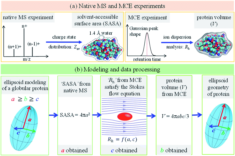
The main concept underlying the method proposed in this work is that the protein geometry, amino acid composition and amino acid sequence determine its charge state distribution in the native mass spectrum, as well as its axial dispersion in the laminar flow of the TDA experiment. As a variant of TDA but with ion separation capability, an MCE experiment was carried out for protein mixture analysis. When no separation electric field was applied, the MCE experiment would reduce to a conventional TDA experiment. Fig. 1 shows the experimental and data analysis procedures to determine the shape of a globular protein. As shown in Fig. 1a, native MS and MCE experiments were carried out to measure the SASA and hydrodynamic radius (Rh) of the target protein, respectively. The shape of a globular protein was approximated as an ellipsoid66 with three independent axes a, b and c (Fig. 1b), in which we assume a ≥ b ≥ c. Experimental results were then fed into the modelling and data processing procedure (Fig. 1b) to acquire the shape of this protein by calculating its ellipsoid radii.
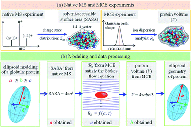 |
| | Fig. 1 Experimental and modeling procedures to characterize the ellipsoid shape of a globular protein. (a) The charge state distribution of a globular protein in its native mass spectrum was used to calculate its SASA, where Zav represents the average charge state. Mobility capillary electrophoresis experiment was carried out to calculate the ion hydrodynamic radius (Rh), which was then used to obtain the protein volume. (b) Ellipsoid modeling and data processing method to determine protein ellipsoid radii (a, b and c). | |
SASA of globular proteins determined by native MS
Theoretical and experimental investigations have shown that the charge state distribution of a protein in the native mass spectrum exhibits a strong dependence on the surface area of its native conformation in solution. It has been found from experiments that a power-law correlation exists between the average charge state of a globular protein (Zav) and its SASA:40| | ln(Zav) = 0.7045![[thin space (1/6-em)]](https://www.rsc.org/images/entities/char_2009.gif) ln(SASA) − 4.1902 ln(SASA) − 4.1902 | (1) |
The average charge state during electrospray is defined as:
| |  | (2) |
where
In represents the signal intensity of the charge state
n. As shown in
Fig. 1a, the SASA of a globular protein could be calculated from the average charge state in its native mass spectrum using
eqn (1).
Protein hydrodynamic radius and volume determined by TDA/MCE
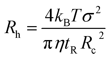
In TDA experiments, the laminar flow occurs within the liquid channel (typically a capillary), and molecular diffusion occurs across the capillary cross section, as well as along the capillary axis. By assuming that diffusion along the capillary axis is negligible, the hydrodynamic radius of a protein (Rh) could be calculated from the Stokes equation:56,67,68| |  | (3) |
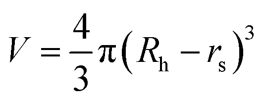
where kB is the Boltzmann constant, T is the temperature in the capillary, Rc is the capillary inner diameter, and η is the viscosity coefficient of the buffer solution. Under controlled experimental conditions, the peak in TDA experiments has a Gaussian shape, and tR and σ2 are the peak arrival time and temporal standard deviation of the protein, respectively. Similarly, the ion hydrodynamic radius could also be obtained from MCE experiments, and details could be found in our previous publications.62–64 The hydrodynamic radius of a protein measured in TDA or MCE experiments includes the thickness of a hydration layer, and the volume of the protein (V) was then estimated as,69| | 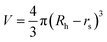 | (4) |
where Rh is in the unit of Angstrom, and rs is the thickness of the hydration layer, which is estimated to be ∼5 Å in accordance with the literature.70,71
Globular protein ellipsoid characterization
As shown in Fig. 1b, the experimental results (SASA, Rh and V) obtained from native MS and MCE could then be utilized to calculate the ellipsoid radii of globular proteins. First, the SASA of a protein in solution is the boundary of atom ball unions, which is different from the geometric surface area of an ellipsoid. Without strong external forces applied, rotational Brownian motions exist for protein ions in solution. As a result, a simple quadratic relationship was found between the SASA of a globular protein and the semi-major axes of its corresponding ellipsoid model:
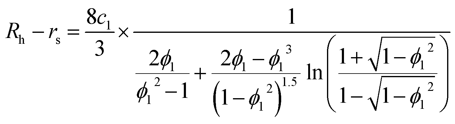
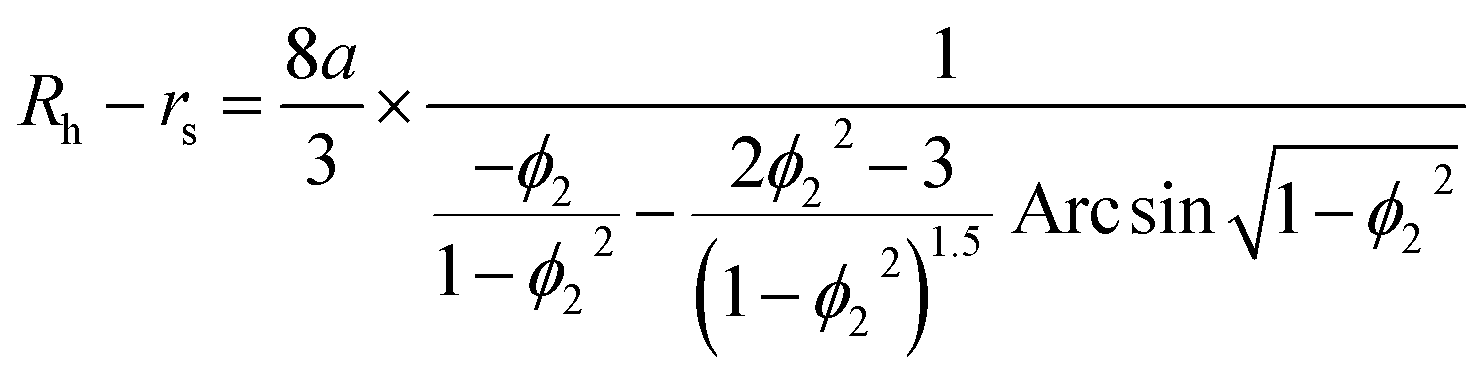
Second, protein ellipsoids flowing in the channel of an MCE experiment need to satisfy the Stokes flow equation. Under MCE experimental conditions, the liquid flow has a low Reynolds number (∼0.07), and the radii of a prolate spheroid (b close or equal to c) should satisfy the following equation,
| | 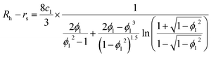 | (6) |
where
ϕ1 =
c1/
a. For an oblate spheroid (
b close or equal to
a), its radii should satisfy:
| | 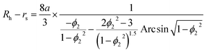 | (7) |
where
ϕ2 =
c2/
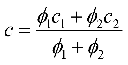
a. In general cases, the smallest radius of the ellipsoid was calculated as a weighted average of these two extreme cases:
| |  | (8) |
With ellipsoid radii
a and
c obtained from
eqn (5) and
(8), respectively, the protein volume information was used to calculate the medium radius of the ellipsoid,
b. The volume of an ellipsoid could be expressed as,
| |  | (9) |
which is equal to that acquired from MCE experiments (
eqn (4)).
Experimental section
Chemicals
All proteins used in this work were purchased from Sigma-Aldrich (St. Louis, MO). Di-sodium hydrogen phosphate (Na2HPO4·12H2O), citric acid monohydrate (C6H8O7·H2O), ammonium acetate (CH3COONH4) and acetic acid (CH3COOH) were purchased from Aldrich Chemical Co. (Milwaukee, WI). Dimethyl sulfoxide (DMSO), phenol, and sodium chloride (NaCl) were obtained from Beijing Chemical Works (Beijing, China). Deionized water was purchased from Wahaha Co. (Hangzhou, China).
TDA/MCE experiment
Both TDA and MCE experiments were performed on a Lumex CE system (model Capel 105 M, St. Petersburg, Russia) equipped with a UV detector (214 nm). The fused silica capillaries of 50 cm total length (75 μm i.d.; 360 μm o.d.) and 40 cm effective length were purchased from Sino Sumtech (Hebei, China). The disodium hydrogen–phosphate citric acid buffers with pH 3.4 and pH 7.0 were prepared by mixing 5.70 mL or 16.47 mL of 0.2 mol L−1 Na2HPO4 with 14.30 mL or 3.53 mL of 0.1 mol L−1 C6H8O7, respectively. At pH 3.4, the final concentrations of phosphate, citric acid, and sodium cations were 57.0 mmol L−1, 71.5 mmol L−1 and 114.0 mmol L−1, respectively. At pH 7.0, the final concentrations of phosphate, citric acid and sodium cations were 164.7 mmol L−1, 17.6 mmol L−1 and 329.4 mmol L−1, respectively. Protein samples were prepared with the buffer to a final protein concentration of 3 mg mL−1. Protein samples for MCE experiments were prepared with a neutral pH buffer containing 2 mmol L−1 NaCl to a final protein concentration of 2 mg mL−1. It should be noticed that the concentration of background ions needs to be at least 10 times higher than that of analyte ions to avoid electromigration dispersion. New coated capillaries (coated with poly N-isopropyl-acrylamide, PAM) were rinsed with water for 30 min before use. The capillaries were flushed sequentially with water (2 min) and running buffer (2 min) before each run. Samples were injected by applying a pressure of 50 mbar for 5 s. A pressure of 50 mbar was then applied across the capillary to maintain the laminar flow within the capillary. The working temperature was set at 25 °C. The difference between TDA and MCE experiments is that a DC separation voltage of −15 kV was applied across the capillary for ion separation in MCE experiments, which induces an electric current of ∼3.6 μA. Samples were run in triplicate.
MS experiment
An Agilent G6520B Accurate-Mass Q-TOF equipped with a standard ESI source was used for the native MS experiments. Protein samples were diluted in water to a final concentration of 1 mg mL−1 with the pH adjusted with 100% acetic acid. A 10 mmol ammonium acetate salt concentration was also maintained in the solvent to preserve the protein structure and facilitate the protein ionization process. According to the literature,39 mass spectra were recorded in the positive ion mode at a constant desolvation plate temperature and at the lowest depolymerization voltage to ensure the consistency of protein ion desorption and transmission conditions.
MD simulations
MD simulations were performed using the GROMOS 54A7 force field (62) (ref. 72) in GROMACS 2016.1.73 The initial structure of lysozyme and BSA was obtained from the PDB data bank (accession numbers: 1GXV and 4F5S, respectively). Acidity constant (pKa) calculations were performed with PROPKA. The systems were placed in a cubic box, solvated with explicit simple point charge (SPC) model water molecules, and neutralized via the replacement of arbitrary solvent with Cl counter-ions.74 The model was then energetically stabilized with the steepest descent algorithm, followed by equilibration for at least 1 ns in water in the NPT ensemble. The overall simulation window was 100 ns. The root-mean-square deviation (RMSD) of the radius of gyration was monitored throughout all simulations.
Results and discussion
Validation of the method
The feasibility of the quadratic relationship (eqn (5)) was verified by testing 52 globular proteins with their molecular weights ranging from 4.7 to 68.7 kDa (Table S1†). The crystal structures of these proteins were extracted from the RCSB Protein Data Bank. The radius of gyration (Rg) of each protein was then extracted to calculate the ellipsoid radii of this protein.75,76 The SASA of each protein was also calculated by using Visual Molecular Dynamics (VMD) by providing protein crystal structures as inputs. The probe radius was set at 1.4 Å for all calculations. After applying eqn (5), the semi-major axis of each protein could be calculated from its corresponding SASA. Fig. 2 plots the correlation between the semi-major axis calculated from the crystal structures extracted from PDB and the semi-major axis calculated from its SASA. A linear correlation was obtained with a slope of 1.0021 and an R square of 0.9514, indicating the feasibility of calculating the protein semi-major axis from its SASA using eqn (5).
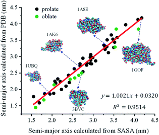 |
| | Fig. 2 The linear correlation between the semi-major axis calculated from protein crystal structures extracted from PDB and the semi-major axis calculated from its SASA. Green dots: oblate proteins; black dots: prolate proteins. | |
Structure determination of different proteins
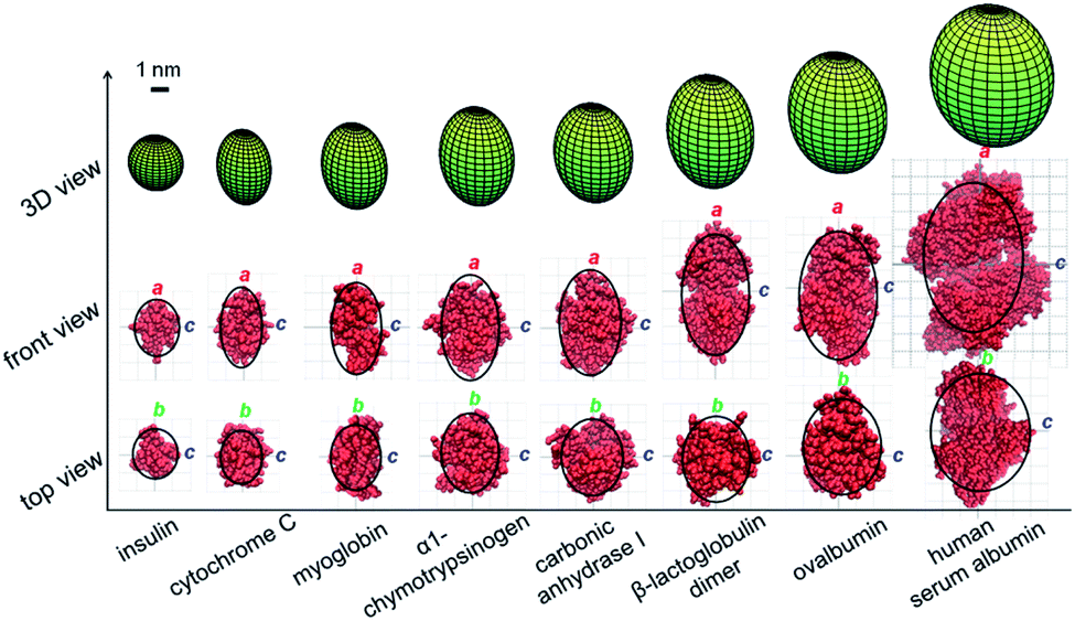
The method proposed in this study was then applied to analyze the shapes of seven globular proteins and a protein dimer under close to physiological conditions. Solvents at pH 7 were used in both native MS and TDA experiments. As shown in Table 1, the average charge states of these proteins were extracted from their native mass spectra in the literature.39 Based on the average charge states (Zav), their corresponding SASAs were calculated using eqn (1) and are shown in Table 1. TDA experiments were then carried out to acquire the hydrodynamic radii of these eight proteins (TDA spectra could be found in Fig. S1†). Eqn (4) was used to calculate the volume of each protein. By applying eqn (5), the semi-major axis (a) of each protein could be calculated based on their corresponding SASA values. By substituting this a value into eqn (6) and (7), two sets of parameters (ϕ1, c1 and ϕ2, c2) used to calculate the smallest radius (c) could be obtained. The smallest radius of the ellipsoid (c) was then obtained from eqn (8). Finally, the protein volume information obtained from eqn (4) was substituted into eqn (9), so that the medium radius (b) could be calculated.
Table 1 Measured and calculated parameters of proteins and a protein complex
| Protein name |
Z
av
|
SASA (nm) |
R
h (nm) |
a (nm) |
c (nm) |
b (nm) |
|
The average charge states of these proteins were extracted from the literature.39
|
| Insulin |
4.40 |
32.38 |
1.90 |
1.58 |
1.25 |
1.39 |
| Cytochrome C |
7.20 |
63.09 |
2.07 |
2.24 |
1.16 |
1.49 |
| Myoglobin |
8.70 |
82.54 |
2.37 |
2.56 |
1.40 |
1.82 |
| Carbonic anhydrase I |
10.54 |
108.37 |
2.71 |
2.94 |
1.72 |
2.13 |
| α1-Chymotrypsinogen |
10.56 |
108.67 |
2.63 |
2.94 |
1.61 |
2.04 |
| β-Lactoglobulin dimer |
12.90 |
144.38 |
2.97 |
3.37 |
1.88 |
2.38 |
| Ovalbumin |
13.89 |
160.35 |
3.24 |
3.57 |
2.17 |
2.66 |
| Human serum albumin |
17.20 |
217.19 |
3.85 |
4.15 |
2.77 |
3.27 |
The ellipsoid geometries of these globular proteins determined using the proposed method were compared to their crystal structures in the PDB database (Fig. 3). The green ellipsoids in the top row are the 3D shapes measured using the proposed method, and the black curves in the middle and bottom rows are the corresponding contour profiles of each ellipsoid. As shown in the middle and bottom rows of Fig. 3, protein crystal structures (red) were fit into the ellipsoid contour profiles for comparison purposes. First, the ellipsoid shape of a single protein could be well characterized in all three dimensions. Nevertheless, the shape of a protein complex, β-lactoglobulin dimer, could also be accurately determined by this method. The agreement achieved for all these proteins and protein complex suggests that the proposed method could be applied as an efficient method to rapidly estimate the shapes of proteins or protein complexes.
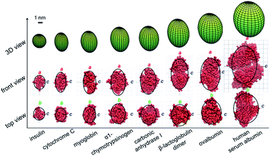 |
| | Fig. 3 Comparison of the ellipsoid shapes of proteins and a protein complex determined by the proposed method (green ellipsoids in the top row; the black curves in the middle and bottom rows are the corresponding contour profiles of each ellipsoid) with their corresponding crystal structures plotted in red (middle and bottom rows). | |
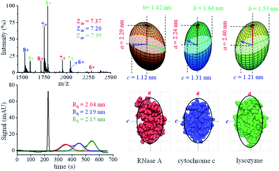
Both native MS and MCE have the capability of mixture analysis, and we thus analyzed a three-protein mixture (ribonuclease A, cytochrome C and lysozyme) prepared in a neutral pH buffer. In the MCE experiment, a neutral marker DMSO (5% v/v) was added to the mixture for calibration purposes.77Fig. 4a shows the native mass spectrum of the three protein mixture, in which the average charge states of ribonuclease A, cytochrome C and lysozyme were determined to be 7.37, 7.20 and 7.95, respectively. The hydrodynamic radii of these proteins were acquired by fitting each peak in the MCE spectrum as shown in Fig. 4b. It should be noticed that Rh obtained in this MCE experiment is within the range from the literature,62 but it is ∼5% larger than those from our TDA experiments (Table 1 and Fig. 4). This is caused by the thermal heating effect of the electric field, which could be minimized by temperature and solvent viscosity corrections.50,63,78,79 After applying the data processing procedure (Fig. 1b), the ellipsoid shapes of these three proteins were determined and are shown in Fig. 4c. The bottom of Fig. 4c also shows the comparison of protein shape results with their corresponding PDB crystal structures.
 |
| | Fig. 4 Analysis of a three-protein mixture. (a) Native mass spectrum. (b) MCE separation of these three proteins. (c) Ellipsoid shapes of these three proteins obtained by the proposed method (top), and comparison with their corresponding crystal structure in the PDB database (bottom) (the black curves are the corresponding contour profiles of each ellipsoid). | |
Structure determination of proteins under different pH conditions
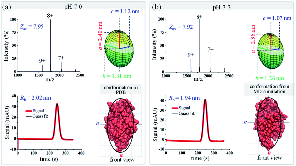
Since protein conformational variations may result in their shape variations, this method could also be applied to distinguish protein conformations. As a proof-of-concept demonstration, protein conformational variations under different pH conditions were explored using this MCE and native MS based method. The shapes of two proteins, lysozyme and bovine serum albumin (BSA), under two pH conditions, pH 7.0 and 3.3, were measured through the combination of TDA and native MS experiments. Fig. 5 shows the native mass spectra and TDA results of lysozyme at pH 7.0 and 3.3. Only minor changes were observed in its charge state distribution (Zav from 7.95 to 7.92) and hydrodynamic radius (from 2.02 to 1.94 nm). The overall shape of lysozyme slightly shrinks, with its ellipsoid radii (a, b, and c) decreasing from (2.40, 1.31, and 1.12) nm to (2.36, 1.26, and 1.07) nm (Fig. 5a top right and Fig. 5b top right). Comparisons between the measured ellipsoid shapes of lysozyme at pH 7.0 and 3.3 with its crystal structure at pH 7.0 and the MD simulated structure at pH 3.3 showed good agreement (Fig. 5). These observations are consistent with previous studies showing that lysozyme could tolerate a wide range of pH and preserve its bioactivity.80,81
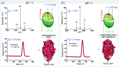 |
| | Fig. 5 Geometric and conformational variations of lysozyme under different pH conditions (a) pH 7.0; (b) pH 3.3. The green ellipsoids (top right in each figure) are the shapes of lysozyme measured by the proposed method. Lysozyme structures (from either the PDB database or MD simulation) are shown in red (bottom right in each figure), and the black curves are the corresponding ellipsoid contour profiles. | |
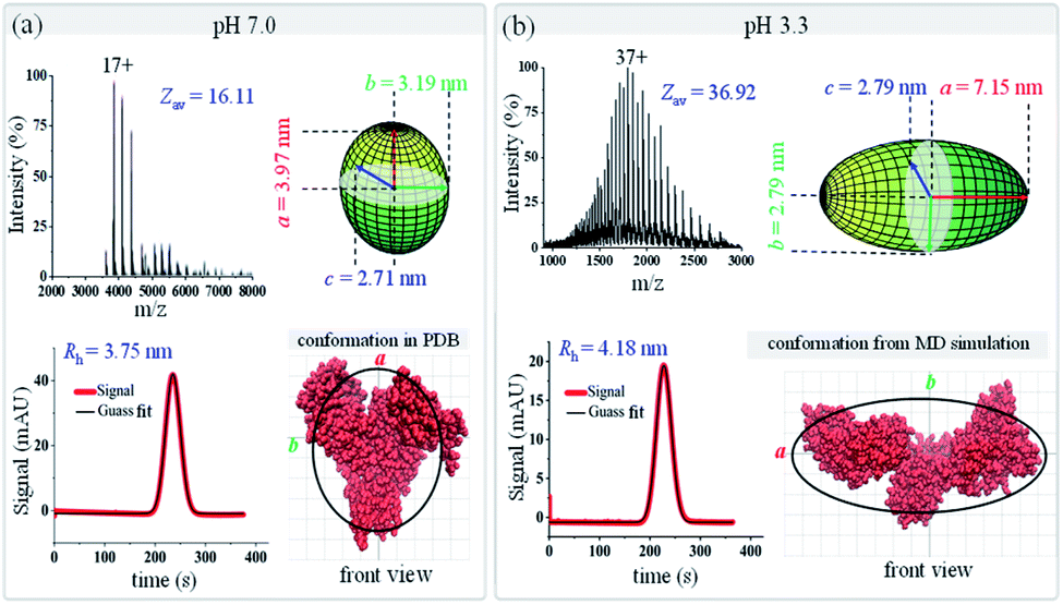
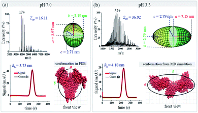
As shown in Fig. 6, dramatic changes are observed for BSA in terms of both its charge state distribution in native mass spectra and its peak width in TDA charts. With decreased pH, the average charge state of BSA shifts from 16.11 up to 36.92, and its hydrodynamic radius increases from 3.75 to 4.18 nm. Following the data analysis procedure in Fig. 1b, the ellipsoid shapes of BSA under these two pH conditions were calculated and are presented in Fig. 6. The results show that BSA has an oblate shape at pH 7.0 with ellipsoid radii of (3.97, 3.19, and 2.71) nm, and it changes to a prolate shape at pH 3.3 with radii of (7.15, 2.79, and 2.79) nm. The crystal structure and MD simulated structure of BSA at pH 7.0 and 3.3 were also plotted on top of the ellipsoid shapes of BSA (bottom right in Fig. 6a and b). With decreased pH, the two branches of BSA would move further away from each other, and BSA would change from a ‘dish’ shape N isoform to an ‘olive’ shape F isoform. Again, the ellipsoid shapes obtained using this native MS and TDA based method agree well with either PDB crystal structures or MD simulation, indicating that this proposed method could be applied to distinguish protein conformational variations. As an important carrier protein which is less likely to aggregate, BSA is often used as an ideal globular protein to study the folding and stretching behaviour of proteins in chemical denaturation. BSA has three primary domains that are arranged in a heart shape with 17 disulfide bond linkages that stabilize these domains.82 BSA can reversibly and drastically change its conformation when exposed to low pH buffers.83,84 Specifically, it has been found that hydrophobic interactions and the helical content within BSA would reduce under low pH conditions, which induces the unfolding of BSA into an “F” conformation,85 consistent with our observations.
 |
| | Fig. 6 Geometric and conformational variations of bovine serum albumin (BSA) under different pH conditions (a) pH 7.0; (b) pH 3.3. The green ellipsoids (top right in each figure) are the shapes of BSA measured by the proposed method. BSA structures (from either the PDB database or MD simulation) are shown in red (bottom right in each figure), and the black curves are the corresponding ellipsoid contour profiles. | |
Conclusions
Here we developed an MCE and native MS based method for the geometric structure determination of globular proteins, which fill the gap between high-throughput proteomics and structural biological techniques. Protein charge state distribution in native MS is correlated with the geometrical parameter of globular proteins or protein complexes. The incorporation of TDA/MCE allows shape determination of globular proteins in a mixture, which is not accessible by conventional technologies. It is true that a protein has complex high-order structures, and even the 3D ellipsoid geometry information is very limited when compared with nuclear magnetic resonance (NMR) or electron microscopy (EM) techniques. Although only low-resolution 3D structure information could be obtained, the MCE and native MS based method is fast in speed, convenient in sample preparation and low in sample consumption. It could also provide complementary protein structure information and has mixture analysis capability. Through individual protein and protein complex shape analyses, this technique could be readily applied to study the formation process of protein complexes. Furthermore, protein conformation and 3D structure information is mostly missing in conventional proteomics approaches. Based on the fact that a fluorescence detector and/or a native mass spectrometer could be integrated with a TDA/MCE instrument directly, improvements of this approach in terms of sensitivity, selectivity and throughput will further increase the potential of incorporating this method in top–down proteomics to identify globular protein stereostructure isomerization. These identified proteins could then be subjected to high-resolution structure analyses by NMR, cryoEM or X-ray crystallography.
Conflicts of interest
There are no conflicts to declare.
Acknowledgements
This work was supported by the NNSFC (21922401, 201827810, and 61635003), National key research and development plan (2018YFF0212503), and Beijing Advanced Innovation Center for Structure Biology.
Notes and references
- I. A. Kaltashov, J. W. Pawlowski, W. Yang, K. Muneeruddin, H. Yao, C. E. Bobst and A. N. Lipatnikov, Methods, 2018, 144, 14–26 CrossRef CAS PubMed.
- A. A. Heemskerk, A. M. Deelder and O. A. Mayboroda, Mass Spectrom. Rev., 2016, 35, 259–271 CrossRef CAS PubMed.
- R. Ramautar, Adv. Clin. Chem., 2016, 74, 1–34 CAS.
- M. Sunde, L. C. Serpell, M. Bartlam, P. E. Fraser, M. B. Pepys and C. C. Blake, J. Mol. Biol., 1997, 273, 729–739 CrossRef CAS PubMed.
- J. S. Fraser, H. van den Bedem, A. J. Samelson, P. T. Lang, J. M. Holton, N. Echols and T. Alber, Proc. Natl. Acad. Sci. U. S. A., 2011, 108, 16247–16252 CrossRef CAS PubMed.
- D. A. Keedy, H. van den Bedem, D. A. Sivak, G. A. Petsko, D. Ringe, M. A. Wilson and J. S. Fraser, Structure, 2014, 22, 899–910 CrossRef CAS PubMed.
- D. J. Hsu, D. Leshchev, D. Rimmerman, J. Hong, M. S. Kelley, I. Kosheleva, X. Zhang and L. X. Chen, Chem. Sci., 2019, 10, 9788–9800 RSC.
- A. J. Baldwin and L. E. Kay, Nat. Chem. Biol., 2009, 5, 808–814 CrossRef CAS PubMed.
- F. A. Mulder, A. Mittermaier, B. Hon, F. W. Dahlquist and L. E. Kay, Nat. Struct. Biol., 2001, 8, 932–935 CrossRef CAS PubMed.
- C. Tang, C. D. Schwieters and G. M. Clore, Nature, 2007, 449, 1078–1082 CrossRef CAS PubMed.
- G. Zhao, J. R. Perilla, E. L. Yufenyuy, X. Meng, B. Chen, J. Ning, J. Ahn, A. M. Gronenborn, K. Schulten, C. Aiken and P. Zhang, Nature, 2013, 497, 643–646 CrossRef CAS PubMed.
- M. Gui, W. Song, H. Zhou, J. Xu, S. Chen, Y. Xiang and X. Wang, Cell Res., 2017, 27, 119–129 CrossRef CAS PubMed.
- J. Xu, M. Gui, D. Wang and Y. Xiang, Nature, 2016, 534, 544–547 CrossRef CAS PubMed.
- A. C. Papageorgiou and J. Mattsson, Methods Mol. Biol., 2014, 1129, 397–421 CrossRef CAS PubMed.
- H. Stark and A. Chari, Microscopy, 2015, 65, 23–34 CrossRef PubMed.
- W. Matthew j and L. L. Andrew, Curr. Protein Pept. Sci., 2009, 10, 116–127 CrossRef PubMed.
- M. R. O'Connell, R. Gamsjaeger and J. P. Mackay, Proteomics, 2009, 9, 5224–5232 CrossRef PubMed.
- E. Nogales and S. H. W. Scheres, Mol. Cell, 2015, 58, 677–689 CrossRef CAS PubMed.
- R.-J. Yu, S.-M. Lu, S.-W. Xu, Y.-J. Li, Q. Xu, Y.-L. Ying and Y.-T. Long, Chem. Sci., 2019, 10, 10728–10732 RSC.
- R.-J. Yu, Y.-L. Ying, R. Gao and Y.-T. Long, Angew. Chem., Int. Ed., 2019, 58, 3706–3714 CrossRef CAS PubMed.
- F.-N. Meng, Y.-L. Ying, J. Yang and Y.-T. Long, Anal. Chem., 2019, 91, 9910–9915 CrossRef CAS PubMed.
- E. C. Yusko, B. R. Bruhn, O. M. Eggenberger, J. Houghtaling, R. C. Rollings, N. C. Walsh, S. Nandivada, M. Pindrus, A. R. Hall, D. Sept, J. Li, D. S. Kalonia and M. Mayer, Nat. Nanotechnol., 2017, 12, 360–367 CrossRef CAS PubMed.
- A. J. Heck, Nat. Methods, 2008, 5, 927–933 CrossRef CAS PubMed.
- R. H. van den Heuvel and A. J. Heck, Curr. Opin. Chem. Biol., 2004, 8, 519–526 CrossRef CAS PubMed.
- J. A. Loo, Mass Spectrom. Rev., 1997, 16, 1–23 CrossRef CAS PubMed.
- E. van Duijn, P. J. Bakkes, R. M. Heeren, R. H. van den Heuvel, H. van Heerikhuizen, S. M. van der Vies and A. J. Heck, Nat. Methods, 2005, 2, 371–376 CrossRef CAS PubMed.
- C. Uetrecht, R. J. Rose, E. van Duijn, K. Lorenzen and A. J. Heck, Chem. Soc. Rev., 2010, 39, 1633–1655 RSC.
- F. Lermyte, D. Valkenborg, J. A. Loo and F. Sobott, Mass Spectrom. Rev., 2018, 37, 750–771 CrossRef CAS PubMed.
- D. Cubrilovic, K. Barylyuk, D. Hofmann, M. J. Walczak, M. Gräber, T. Berg, G. Wider and R. Zenobi, Chem. Sci., 2014, 5, 2794–2803 RSC.
- H. Li, H. H. Nguyen, R. R. Ogorzalek Loo, I. D. G. Campuzano and J. A. Loo, Nat. Chem., 2018, 10, 139–148 CrossRef CAS PubMed.
- A. Politis, F. Stengel, Z. Hall, H. Hernandez, A. Leitner, T. Walzthoeni, C. V. Robinson and R. Aebersold, Nat. Methods, 2014, 11, 403–406 CrossRef CAS PubMed.
- J. Gault, J. A. Donlan, I. Liko, J. T. Hopper, K. Gupta, N. G. Housden, W. B. Struwe, M. T. Marty, T. Mize, C. Bechara, Y. Zhu, B. Wu, C. Kleanthous, M. Belov, E. Damoc, A. Makarov and C. V. Robinson, Nat. Methods, 2016, 13, 333–336 CrossRef PubMed.
- J. Snijder, R. J. Rose, D. Veesler, J. E. Johnson and A. J. Heck, Angew. Chem., Int. Ed. Engl., 2013, 52, 4020–4023 CrossRef CAS.
- M. van de Waterbeemd, K. L. Fort, D. Boll, M. Reinhardt-Szyba and A. Routh, Nat. Methods, 2017, 14, 283–286 CrossRef CAS PubMed.
- S. Rosati, Y. Yang, A. Barendregt and A. J. Heck, Nat. Protoc., 2014, 9, 967–976 CrossRef CAS PubMed.
- C. Schmidt and C. V. Robinson, Nat. Protoc., 2014, 9, 2224–2236 CrossRef CAS PubMed.
- N. A. Yewdall, T. M. Allison, F. G. Pearce, C. V. Robinson and J. A. Gerrard, Chem. Sci., 2018, 9, 6099–6106 RSC.
- I. A. Kaltashov and A. Mohimen, Anal. Chem., 2005, 77, 5370–5379 CrossRef CAS PubMed.
- L. Testa, S. Brocca and R. Grandori, Anal. Chem., 2011, 83, 6459–6463 CrossRef CAS PubMed.
- Z. Hall and C. V. Robinson, J. Am. Soc. Mass Spectrom., 2012, 23, 1161–1168 CrossRef CAS PubMed.
- A. Natalello, C. Santambrogio and R. Grandori, J. Am. Soc. Mass Spectrom., 2017, 28, 21–28 CrossRef CAS PubMed.
- J. Li, C. Santambrogio, S. Brocca, G. Rossetti, P. Carloni and R. Grandori, Mass Spectrom. Rev., 2016, 35, 111–122 CrossRef CAS PubMed.
- Z. Hall, A. Politis and C. V. Robinson, Structure, 2012, 20, 1596–1609 CrossRef CAS PubMed.
- B. T. Ruotolo, J. L. P. Benesch, A. M. Sandercock, S.-J. Hyung and C. V. Robinson, Nat. Protoc., 2008, 3, 1139–1152 CrossRef CAS PubMed.
- G. Li, S. Zheng, Y. Chen, Z. Hou and G. Huang, Anal. Chem., 2018, 90, 7997–8001 CrossRef CAS PubMed.
- J. Fan, P. Lian, M. Li, X. Liu, X. Zhou and Z. Ouyang, Anal. Chem., 2020, 92, 2573–2579 CrossRef CAS PubMed.
- V. Domalain, M. Hubert-Roux, V. Tognetti, L. Joubert, C. M. Lange, J. Rouden and C. Afonso, Chem. Sci., 2014, 5, 3234–3239 RSC.
- J. C. May, C. B. Morris and J. A. McLean, Anal. Chem., 2017, 89, 1032–1044 CrossRef CAS PubMed.
- J. N. Dodds and E. S. Baker, J. Am. Soc. Mass Spectrom., 2019, 30, 2185–2195 CrossRef CAS PubMed.
- J. Sun, E. N. Kitova, W. Wang and J. S. Klassen, Anal. Chem., 2006, 78, 3010–3018 CrossRef CAS PubMed.
- F. Wang, M. A. Freitas, A. G. Marshall and B. D. Sykes, Int. J. Mass Spectrom., 1999, 192, 319–325 CrossRef CAS.
- G. Taylor, The Dispersion of Soluble Matter in Solvent Flowing Slowly Through a Tube, Proc. R. Soc. London, Ser. A, 1953, 219, 186–203 CAS.
- R. Aris, On the Dispersion of a Solute in a Fluid Flowing through a Tube, Proc. R. Soc. London, Ser. A, 1956, 235, 67–77 Search PubMed.
- F. Oukacine, A. Geze, L. Choisnard, J. L. Putaux, J. P. Stahl and E. Peyrin, Anal. Chem., 2018, 90, 2493–2500 CrossRef CAS PubMed.
- S. Balog, Anal. Chem., 2018, 90, 4258–4262 CrossRef CAS PubMed.
- J. Ostergaard and H. Jensen, Anal. Chem., 2009, 81, 8644–8648 CrossRef PubMed.
- W. L. Hulse, J. Gray and R. T. Forbes, Int. J. Pharm., 2013, 453, 351–357 CrossRef CAS PubMed.
- E. G. Alexov and M. R. Gunner, Biophys. J., 1997, 72, 2075–2093 CrossRef CAS PubMed.
- J. Chamieh, D. Koval, A. Besson, V. Kašička and H. Cottet, J. Chromatogr. A, 2014, 1370, 255–262 CrossRef CAS PubMed.
- A. Ibrahim, D. Koval, V. Kašička, C. Faye and H. Cottet, Macromolecules, 2013, 46, 533–540 CrossRef CAS.
- T. Tůmová, L. Monincová, O. Nešuta, V. Čeřovský and V. Kašička, Electrophoresis, 2017, 38, 2018–2024 CrossRef PubMed.
- R. Zhang, H. Wu, M. He, W. Zhang and W. Xu, J. Phys. Chem. B, 2019, 123, 2335–2341 CrossRef CAS PubMed.
- W. Zhang, H. Wu, R. Zhang, X. Fang and W. Xu, Chem. Sci., 2019, 10, 7779–7787 RSC.
- M. He, P. Luo, J. Hong, X. Wang and W. Xu, ACS Omega, 2019, 4, 2377–2386 CrossRef CAS PubMed.
- H. Yang, S. Yang, J. Kong, A. Dong and S. Yu, Nat. Protoc., 2015, 10, 382–396 CrossRef CAS PubMed.
- W. R. Taylor, J. Thornton and W. G. Turnell, J. Mol. Graphics, 1983, 1, 30–38 CrossRef CAS.
- U. Sharma, N. J. Gleason and J. D. Carbeck, Anal. Chem., 2005, 77, 806–813 CrossRef CAS PubMed.
- F. Oukacine, A. Morel, I. Desvignes and H. Cottet, J. Chromatogr. A, 2015, 1426, 220–225 CrossRef CAS PubMed.
- H. F. Fisher, Proc. Natl. Acad. Sci. U. S. A., 1964, 51, 1285–1291 CrossRef CAS PubMed.
- S. K. Sinha, S. Chakraborty and S. Bandyopadhyay, J. Phys. Chem. B, 2008, 112, 8203–8209 CrossRef CAS PubMed.
- S. Pal and S. Bandyopadhyay, J. Phys. Chem. B, 2013, 117, 5848–5856 CrossRef CAS PubMed.
- N. Schmid, A. P. Eichenberger, A. Choutko, S. Riniker, M. Winger, A. E. Mark and W. F. van Gunsteren, Eur. Biophys. J., 2011, 40, 843–856 CrossRef CAS PubMed.
- M. Abraham, T. Murtola, R. Schulz, S. Páll, J. Smith, B. Hess and E. Lindahl, SoftwareX, 2015, 1–2, 19–25 CrossRef.
- T. A. Soares, X. Daura, C. Oostenbrink, L. J. Smith and W. F. van Gunsteren, J. Biomol. NMR, 2004, 30, 407–422 CrossRef CAS PubMed.
- A. S. Seshasayee, Theor. Biol. Med. Modell., 2005, 2, 7 CrossRef PubMed.
- P. Mittelbach and G. Porod, Colloid Polym. Sci., 1965, 202, 40–49 CrossRef CAS.
- A. Hellqvist, Y. Hedeland and C. Pettersson, Electrophoresis, 2013, 34, 3252–3259 CrossRef CAS PubMed.
- G. Y. Tang, C. Yang, H. Q. Gong, J. Chai and Y. C. Lam, Anal. Chim. Acta, 2006, 561, 138–149 CrossRef CAS.
- J. Vlassakis and A. E Herr, Anal. Chem., 2017, 89, 12787–12796 CrossRef CAS PubMed.
- K. Ogasahara and K. Hamaguchi, J. Biochem., 1967, 61, 199–210 CrossRef CAS PubMed.
- A. Bonincontro, A. De Francesco and G. Onori, Colloids Surf., B, 1998, 12, 1–5 CrossRef CAS.
-
T. Peters, in All About Albumin, ed. T. Peters, Academic Press, San Diego, 1995, pp. 9–75 Search PubMed.
- C. Leggio, L. Galantini and N. V. Pavel, Phys. Chem. Chem. Phys., 2008, 10, 6741–6750 RSC.
- K. Baler, O. A. Martin, M. A. Carignano, G. A. Ameer, J. A. Vila and I. Szleifer, J. Phys. Chem. B, 2014, 118, 921–930 CrossRef CAS PubMed.
- L. M. Clark, Gut, 1978, 19, 159 CrossRef.
Footnotes |
| † Electronic supplementary information (ESI) available. See DOI: 10.1039/d0sc01965h |
| ‡ These authors contributed equally to this work. |
|
| This journal is © The Royal Society of Chemistry 2020 |
Click here to see how this site uses Cookies. View our privacy policy here. 
 Open Access Article
 This Open Access Article is licensed under a Creative Commons Attribution-Non Commercial 3.0 Unported Licence
 *a
*a