Dynamic contrast with reversibly photoswitchable fluorescent labels for imaging living cells

Abstract

Interrogating living cells requires sensitive imaging of a large number of components in real time. The state-of-the-art of multiplexed imaging is usually limited to a few components. This review reports on the promise and the challenges of dynamic contrast to overcome this limitation.

---

Deciphering living matter

Living matter has continuously fascinated chemists. Reproducing its structural elements and functions has motivated and challenged organic, supramolecular, and systems chemists. Powerful analytical tools are also required for its interrogation.

Cells as complex media

Living cells significantly depart from the material organization encountered by chemists in their current practice: (i) they contain a large number of distinct components (more than 10⁶); (ii) the molar concentrations of their components span an extremely large dynamic range (from 10⁻¹ mol L⁻¹ for ions such as Na⁺, K⁺, or Cl⁻, to 10⁻¹² mol L⁻¹ for DNA); (iii) they exhibit multi-scale space heterogeneity and time dynamics in the steady state. Their components are heterogeneously but precisely distributed in space. The genome is more or less static, the transcriptome and the proteome evolve on a time scale of minutes to hours, the metabolome fluctuates on the second time scale, and membrane (de)polarization occurs on the millisecond time scale; (iv) they are in an out-of-equilibrium (living) state. As a consequence, meaningfully interrogating living cells requires sensitive imaging of a large number of components in “real time”. Fulfilling such a goal is a source of multiple chemical challenges.

Imaging cells as a source of challenges

Selective labeling. Imaging a cell component requires a specific signature, which is read out with an interrogating tool (e.g. light). Moreover, cell components essentially share a similar elemental composition and functional groups, which hinders the discrimination of a target among the population of biomolecules. To overcome this limitation, exogenous labels (e.g. fluorophores) are often introduced to singularize a target. Powerful technologies (involving genetic modification to introduce a derivatizable tag or a labeled brick) have been developed to introduce such labels into biomolecules,^1–3 so imaging is presently limited by label discrimination.

Sensitivity at its limits. The sensitivity of an observable is associated with the minimal label concentration which can be detected in a given time. The most sensitive observables (e.g. fluorescence) currently give access to submicromolar concentrations at a 100 Hz frequency of image acquisition. Such a detection level is at the limits required for real time imaging of key cell factors such as transcription factors or RNA molecules. Strategies of signal amplifications relying on reaction cascades⁴ or labeling with enzymes⁵ are currently under development.

Overcoming adverse conditions. The heterogeneity of living matter causes differential absorption and light scattering.⁶ Cells may also contain spectrally active endogenous components (e.g. giving rise to autofluorescence⁷). Both features are detrimental to unambiguously retrieving the label signals. The development of strategies aiming at overcoming the interference of the latter phenomena for quantitative and spatially informative interpretation is a field of active research (e.g. tissue clearing,⁸ labels emitting chemiluminescence,^9,10 bioluminescence¹¹ or fluorescence in the near infrared region, where autofluorescence is weak¹²).

Multiplexed observations. Selectivity for imaging is governed by the ratio of the bandwidth of the label signal and the range of all possible signals. No spectroscopy is presently able to image a large number of cell components at their actual concentrations. In fluorescence imaging which benefits from high sensitivity and versatility for labeling, this ratio is at the lowest equal to 0.25 with an organic label (e.g. in a fluorescent protein), which enables the discrimination of 4 fluorophores in the UV-visible wavelength range by using spectral filters. This ratio can reach down to 0.01 in Raman spectroscopy, which should give access to imaging up to 100 labels.¹³

Spectral discrimination versus dynamic contrast for imaging

Spectral discrimination at its limits

In imaging, the common approach to discriminate a label from its background is to read out its signal in the spectral domain. In particular, it has found extensive use in fluorescence imaging, which has become essential for biology in view of the high sensitivity and versatility of fluorescence for labeling.¹⁴ Two discriminative dimensions – the excitation and emission wavelengths – can be exploited to target a specific fluorescent label. Yet, the 50–100 nm half-width of the absorption/emission bands of the widely used fluorophores intrinsically limits spectral discrimination. Even with rich hardware of light sources and optical devices, at most four labels can be distinguished. Further increasing this number requires spectral unmixing but at significant cost in terms of photon budget and computation time.^15–22 Such constraints currently limit the discriminative power of emerging genetic engineering strategies,^23–25 which can already be implemented to label a larger number of biomolecules or cells in order to interrogate signaling pathways,²⁶ cycling states,²⁷ genotypes,^28,29 neuronal projections,^23,30,31 clones,^26–33 cell types,³⁴ or microbiomes.³⁵ Since fluorescence should remain a much favored observable for imaging live cells,³⁶ the spectral dimension has to be complemented by another dimension for further discriminating fluorophores (see Fig. 1a and b).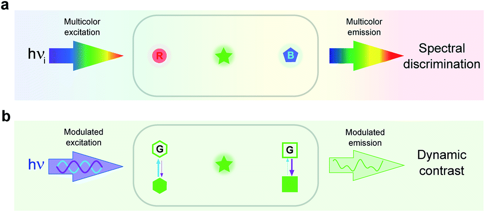

Fig. 1 Complementary spectral (a) and dynamic (b) dimensions for label discrimination. Spectral discrimination uses the responses of labels submitted to spectrally different conditions of illumination and light collection. Dynamic discrimination of spectrally similar labels exploits their time responses to the change of control parameters (e.g. light intensity). The spectral and dynamic discriminations exploit two orthogonal dimensions. They can be combined in order to further expand the number of labels, which can be discriminated in imaging. Fluorescence has been used here for illustration. In (a), R, G, and B respectively denote red, green, and blue absorbing/emitting fluorophores, which can be distinguished by means of optical filters. In (b), two RSFs engaged in reversible fluorescence photoswitching driven at two wavelengths (indicated by blue and violet arrows) with different photoswitching cross sections can be discriminated after the analysis of the modulated fluorescence emission resulting from the application of modulated light excitation.

State of the art of dynamic contrast

Chemists have a lot of experience in adding discriminative functions to reporters. In titrations, they selectively probe analytes by means of the thermodynamic and kinetic aspects of their reaction with specific labeled reagents.³⁷ Interestingly fluorescence emission precisely reports on a photocycle of reactions including light absorption and relaxation pathways from an excited state, which can be envisioned as a titrating set. As such, it contains a wealth of dynamic information, which can be used for discrimination beyond the sole wavelength of its emission.

Spectrally overlapping fluorophores have been discriminated earlier by using their absorption–fluorescence emission photocycle. In particular the lifetime of excited states has been exploited to distinguish fluorophores in Fluorescence Lifetime Imaging Microscopy (FLIM).^38,39 However this original attempt has been limited by the narrow lifetime dispersion (less than an order of magnitude in the ns range) of the bright fluorophores currently used in fluorescence imaging. Therefore multiplexed fluorescence lifetime imaging has necessitated deconvolutions⁴⁰ or the adoption of subtraction schemes.³⁸

Reversibly photoswitchable fluorophores (RSFs) do not suffer from this drawback. These labels benefit from photochemistry, which goes much beyond the absorption–fluorescence emission photocycle. It results in relaxation times of fluorescence photoswitching on timescales necessitating simpler setups than in FLIM while remaining compatible with real time observations of biological phenomena. Thus several protocols (e.g. optical lock-in detection – OLID,⁴¹ synchronously amplified fluorescence image recovery – SAFIRe,^42,43, transient state imaging microscopy – TRAST,⁴⁴ and out-of-phase imaging after optical modulation – OPIOM^45–48) have exploited the time response of fluorescence to light variations for discriminating up to three spectrally similar RSFs,⁴⁶ by relying on neither deconvolution nor subtraction schemes.

Eventually Bleaching-Assisted Multichannel Microscopy (BAMM) exploits the specific kinetic signature of photobleaching, which has made possible the discrimination of up to three spectrally similar fluorophores with an unmixing algorithm.⁴⁹

Out-of-phase imaging after optical modulation (OPIOM)

We more specifically report on the OPIOM protocol, which has been introduced for RSF imaging. In OPIOM, the dynamic contrast is obtained by applying modulated illumination at a specific angular frequency and reading out the amplitude of the modulated fluorescence signal.

In the one-color version of OPIOM, illumination at one wavelength (intensity I) drives RSF photoswitching between two states 1 and 2 of distinct brightness (see Fig. 2a).^45,50 The thermodynamically stable state 1 is photochemically depopulated toward the thermodynamically unstable state 2 with a rate constant k₁₂(t) = σ₁₂I(t). State 1 is populated back either by photochemical induction or thermal recovery with a rate constant k₂₁(t) = σ₂₁I(t) + k^Δ₂₁. σ₁₂ and σ₂₁ are the photoswitching action cross sections of the RSF, and k^Δ₂₁ is the rate constant for the thermal recovery of 1 from 2. Since the photoswitching rates are proportional to the light intensity I(t), its sinusoidal modulation at mean intensity (I⁰) and angular frequency (ω) harmonically modulates the concentrations of the two RSF states at the angular frequency ω but with a phase lag. Interestingly the in-phase and quadrature amplitudes of the modulated concentrations depend on I⁰ and on ω. In particular, the quadrature amplitude exhibits a resonance with a single optimum when the control parameters (I⁰, ω) fulfill two conditions:

ω = 2k^Δ₂₁ (2)

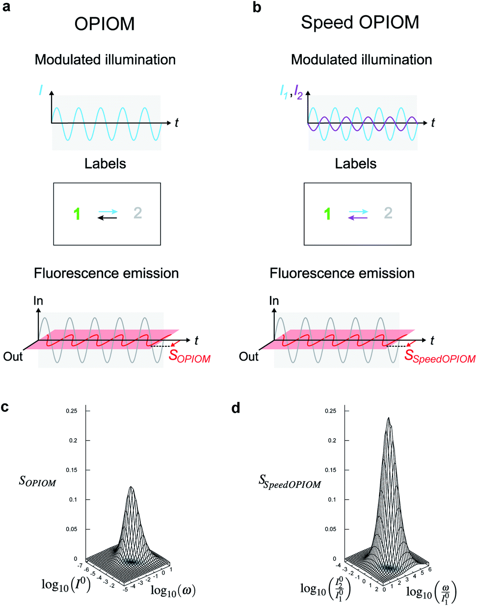Fig. 2 Principle of (Speed) out-of-phase imaging after optical modulation (OPIOM). (a and c) In OPIOM, a periodically modulated light source (angular frequency ω and average intensity I⁰) modulates the fluorescence emission from a RSF exchanging between two states (1 and 2) having different brightness (a). The OPIOM signal S_OPIOM is the amplitude of the quadrature component of the modulated fluorescence emission, which exhibits a resonance in the space of the illumination parameters (I⁰, ω) (c). The OPIOM image of a targeted RSF is selectively and quantitatively retrieved at resonance upon relating I⁰ and ω to its dynamic parameters σ₁₂, σ₂₁, and k^Δ₂₁ using the resonance conditions (1, 2); (b and d) in Speed-OPIOM, the periodically modulated illumination involves two light sources modulated in an antiphase at angular frequency ω with respective average light intensities I⁰₁ and I⁰₂ (b). The Speed OPIOM signal S_SpeedOPIOM is the amplitude of the quadrature component of the modulated fluorescence emission. It exhibits a resonance in the space of the illumination parameters (I⁰₂/I⁰₁ and ω/I⁰₁) (d). The Speed OPIOM image of a targeted RSF is obtained after relating I⁰₂/I⁰₁ and ω/I⁰₁ to its dynamic parameters σ_12,1, σ_21,1, σ_12,2, and σ_21,2 using the resonance conditions (3, 4). The theoretical plots in (c) and (d) have been computed with σ₁₂ = σ_12,1 = 196 m² mol⁻¹, σ_21,1 = σ_12,2 = 0 m² mol⁻¹, σ₂₁ = σ_21,2 = 413 m² mol⁻¹, k^Δ₂₁ = 1.5 × 10⁻² s⁻¹ and I⁰₁ = 100(k^Δ₂₁/σ_12,1 + σ_21,1) in (d).

The fluorescence emission exhibits a similar resonant behavior with identical resonance conditions. Hence the out-of-phase amplitude of the modulated fluorescence has been adopted as the OPIOM signal (see Fig. 2c). Proportional to the RSF concentration, it is simply extracted by time Fourier transform thereby benefiting from lock-in amplification, which improves the signal-to-noise ratio. Since the resonance conditions (1, 2) are specific for a RSF defined by its features of fluorescence photoswitching, OPIOM can discriminate a targeted RSF from autofluorescence, a spectrally similar fluorophore, or another RSF endowed with distinct photoswitching kinetics. OPIOM has been experimentally validated by selective imaging of green reversibly photoswitchable fluorescent proteins (RSFPs⁵¹) in microsystems, mammalian cells, and in zebrafish by using a wide-field epifluorescence microscope or a single plane illumination microscope.⁴⁵

In its original implementation, OPIOM has suffered from too low values of the rate constant k^Δ₂₁ for thermal recovery of photoswitched RSFPs. Even with the fastest recovering RSFP (Dronpa-3), OPIOM image acquisition took more than 2 min.⁴⁵ Since most photoswitched green RSFPs can be photoswitched back to their stable state upon illumination at 405 nm, it has been proposed that the preceding limitation can be overcome by introducing a secondary light source at 405 nm in order to accelerate the recovery process.^46,52

In the advanced Speed OPIOM protocol exploiting periodic two-color illumination, the light sources at 480 and 405 nm are modulated in an antiphase at the same angular frequency ω with the respective average light intensities I⁰₁ and I⁰₂ (see Fig. 2b).⁴⁶ The RSFP fluorescence signal exhibits a tunable quadrature response with a single resonance in the space of the illumination parameters (I⁰₂/I⁰₁ and ω/I⁰₁) (see Fig. 2). The resonant values are determined by the RSFP photoswitching cross sections σ_12,i (σ_21,i respectively) associated with photoswitching from 1 to 2 (from 2 to 1 respectively) driven at 480 (i = 1) and 405 (i = 2) nm

(σ_12,1 + σ_21,1)I⁰₁ = (σ_12,2 + σ_21,2)I⁰₂ (3)

ω = 2(σ_12,1 + σ_21,1)I⁰₁. (4)

The Speed OPIOM signal is two-times higher than the one obtained in the original one-color OPIOM.⁴⁶ Moreover, the resonance conditions (3, 4) show that the light sources can be modulated at a much higher angular frequency than in one-color OPIOM. Increasing I⁰₁ and I⁰₂ upon keeping their ratio constant allows one to shorten the imaging time down to the millisecond scale.

Experimental validations evidenced that Speed OPIOM can quantitatively image RSFs against a background of autofluorescence (see Fig. 3a and b) or ambient light.⁴⁶ It is as well efficient for multiplexed fluorescence imaging. Indeed by using Speed OPIOM we could independently image at the Hz frequency of image acquisition three spectrally similar RSFPs having different responses to light modulation.⁴⁶ Speed OPIOM proved relevant for macroscale fluorescence, which is increasingly used to observe biological samples.⁴⁷ In particular, it enhanced the sensitivity and the signal-to-noise ratio for fluorescence detection in blot assays by factors of 50 and 10, respectively, over direct fluorescence observation under constant illumination. Moreover it easily discriminated fluorescent labels from the autofluorescence and reflective background in labeled leaves of plant seedlings, even under the interference of incident light at intensities that are comparable to that of sunlight. Speed OPIOM has also been implemented in fiber-optic epifluorescence imaging with one-photon excitation.⁴⁸ Besides demonstrating that it efficiently eliminates the interference of autofluorescence arising from both the fiber bundle and the specimen in several biological samples, we showed that it provides intrinsic optical sectioning. This favorable feature restricts the observation of fluorescent labels at targeted positions within a sample thereby eliminating the out-of-focus background, which generally results in low-contrast images.

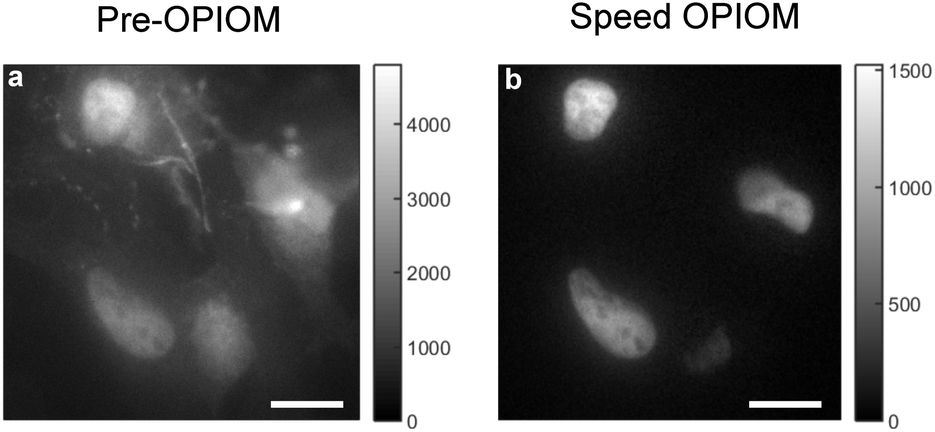Fig. 3 Speed OPIOM in action. (a and b) Fixed HeLa cells expressing H2B-Dronpa-2 (in the nucleus) and Lyn11-EGFP (at the cell membrane). Pre-OPIOM (a) and Speed OPIOM (b) images obtained from analyzing a movie recorded at 525 nm under sinusoidal illumination modulation at a single radial frequency tuned at the resonance of Dronpa-2 (λ_exc,1; I⁰₁; ω) = (480 nm; 3.2 × 10⁻² Ein m⁻² s⁻¹; 12.5 rad s⁻¹ or 2 Hz) and (λ_exc,2; I⁰₂; ω) = (405 nm; 1.5 × 10⁻² Ein m⁻² s⁻¹; 12.5 rad s⁻¹ or 2 Hz). The experiments were performed at 25 °C. Dronpa-2 fluorescence emission is detected in both pre-OPIOM (a) and Speed OPIOM (b) images. In contrast, as expected from the absence of an out-of-phase contribution in its fluorescence emission, the EGFP gives a signal on the pre-OPIOM image (a) but not on the Speed OPIOM one (b). Scale bars: 10 μm.

Dynamic contrast as a frontier for chemists

Despite the work of chemists, the labels and protocols for imaging are still far from meeting the growing demand of quantitative biology to simultaneously image tens of chemical species in a cell or nearby cells within a tissue.^53,54 Since the optimization of the spectral features of labels (e.g. in fluorescence imaging: cross sections for light absorption, quantum yield of luminescence, and half-width of absorption/emission bands) has essentially reached its physical limits,³⁶ it is timely to complement the spectral dimension. As has been illustrated in the preceding paragraphs, dynamic contrast can provide attractive opportunities. Yet, until now, it has not enabled the discrimination of more than a few labels. However, in contrast to spectral discrimination which has benefited from a century of developments, much can be done in order to improve the dynamic contrast. In the following, we present a few of its frontiers with emphasis on fluorescence as an observable.

New labels

Most presently available fluorophores and RSFs have not been specifically designed for dynamic contrast. As such, they are not necessarily optimal for the specific figures of merits required for the various protocols of dynamic contrast. This situation will encourage tailoring labels endowed with optimized kinetic properties (e.g. luminescence lifetimes, cross sections for luminescence photoswitching, etc.). For instance, long-lived luminophores can be sought (e.g. lanthanide-based luminescent probes,⁵⁵ azadioxatriangulenium (ADOTA) fluorophores,^56,57 and Ag clusters⁵⁸). Similarly, RSFPs endowed with diverse cross sections for fluorescence photoswitching should be developed.

New observables

The development of dynamic contrast should not be limited to the syntheses of new labels and to their integration with living matter. In fact, it will be also necessary to engage theoretical and instrumental efforts in order to introduce new acquisition protocols. Another interesting development concerns the design of observables. For a simple label, the observable (e.g. the intensity of the fluorescence signal) reports on its instantaneous concentration. Hence, it is necessary to record successive images to reconstruct the temporal evolution of a dynamic system. In addition, to obtain three-dimensional images at the highest spatial resolution, this approach necessitates acquisition, processing, and storage of huge amounts of information, which is difficult with organs or organisms and represents a bottleneck in bioimaging. As a promising avenue to overcome the preceding limitation, new labels acting as integrators have been recently proposed to report not on a single state but on a succession of states delivering time information in a compact format.⁵⁹

Concluding remarks

We end up this mini-review with a more general consideration. The field of methodological developments in imaging cannot be easily addressed at the level of one research group only. Indeed it necessitates to integrate theoretical and instrumental developments, systems and labels, together with taking into account scientific questions from remote communities. In our experience, this requirement proved highly rewarding by offering opportunities of rich interactions with scientists from other disciplines (physicists, biologists, data scientists, …). Added to the preceding considerations showing that much has to be done, we are therefore convinced that imaging living matter will deserve much attention from the community of chemists.

Conflicts of interest

There are no conflicts to declare.

Acknowledgements

This work was supported by the ANR (France BioImaging – ANR-10-INBS-04, Morphoscope2 – ANR-11-EQPX-0029, HIGHLIGHT, and dISCern), the Fondation de la Recherche Médicale (FRM), and the MITI CNRS (Imag'In and Instrumentations aux limites).

Notes and references

1. K. M. Marks and G. P. Nolan, Nat. Methods, 2006, 3, 591.
2. K. M. Dean and A. E. Palmer, Nat. Chem. Biol., 2014, 10, 512.
3. E. A. Specht, E. Braselmann and A. E. Palmer, Annu. Rev. Physiol., 2017, 79, 93–117.
4. X. Sun, D. Shabat, S. T. Phillips and E. V. Anslyn, J. Phys. Org. Chem., 2018, 31, e3827.
5. A. P. Demchenko, Introduction to fluorescence sensing, Springer Science & Business Media, 2008.
6. S. L. Jacques, Phys. Med. Biol., 2013, 58, R37.
7. A. C. Croce and G. Bottiroli, Eur. J. Histochem., 2014, 58, 320–337.
8. D. S. Richardson and J. W. Lichtman, Cell, 2015, 162, 246–257.
9. N. Hananya and D. Shabat, ACS Cent. Sci., 2019, 5, 949–959.
10. Q. Li, J. Zeng, Q. Miao and M. Gao, Front. Bioeng. Biotech., 2019, 7, 326.
11. A. Fleiss and K. S. Sarkisyan, Curr. Genet., 2019, 1–6.
12. G. Hong, A. L. Antaris and H. Dai, Nat. Biomed. Eng., 2017, 1, 0010.
13. L. Wei, Z. Chen, L. Shi, R. Long, A. V. Anzalone, L. Zhang, F. Hu, R. Yuste, V. W. Cornish and W. Min, Nature, 2017, 544, 465.
14. B. N. G. Giepmans, S. R. Adams, M. H. Ellisman and R. Y. Tsien, Science, 2006, 312, 217–224.
15. T. Zimmermann, J. Rietdorf and R. Pepperkok, FEBS Lett., 2003, 546, 87–92.
16. R. Neher and E. Neher, J. Microsc., 2004, 213, 46–62.
17. J. R. Mansfield, K. W. Gossage, C. C. Hoyt and R. M. Levenson, J. Biomed. Opt., 2005, 104, 041207.
18. L. Gao and R. T. Smith, J. Biophotonics, 2014, 1–16.
19. W. Jahr, B. Schmid, C. Schmied, F. O. Fahrbach and J. Huisken, Nat. Commun., 2015, 6, 7990.
20. A. M. Valm, J. L. M. Welch, C. W. Rieken, Y. Hasegawa, M. L. Sogin, R. Oldenbourg, F. E. Dewhirst and G. G. Borisy, Proc. Natl. Acad. Sci. U. S. A., 2011, 108, 4152–4157.
21. F. Cutrale, V. Trivedi, L. A. Trinh, C.-L. Chiu, J. M. Choi, M. S. Artiga and S. E. Fraser, Nat. Methods, 2017, 14, 149–152.
22. A. Valm, S. Cohen, W. Legant, J. Melunis, U. Hershberg, E. Wait, A. Cohen, M. Davidson, E. Betzig and J. Lippincott-Schwartz, Nature, 2017, 546, 162–167.
23. J. Livet, T. A. Weissman, H. Kang, R. W. Draft, J. Lu, R. A. Bennis, J. R. Sanes and J. W. Lichtman, Nature, 2007, 450, 56–62.
24. M. Mansouri, I. Bellon-Echeverria, A. Rizk, Z. Ehsaei, C. C. Cosentino, C. S. Silva, Y. Xie, F. M. Boyce, M. W. Davis and S. C. Neuhauss, et al. , Nat. Commun., 2016, 7, 11529.
25. Y. Cai, M. J. Hossain, J.-K. Hériché, A. Z. Politi, N. Walther, B. Koch, M. Wachsmuth, B. Nijmeijer, M. Kueblbeck and M. Martinic-Kavur, et al. , Nature, 2018, 561, 411.
26. S. Regot, J. J. Hughey, B. T. Bajar, S. Carrasco and M. W. Covert, Cell, 2014, 157, 1724–1734.
27. B. T. Bajar, A. J. Lam, R. K. Badiee, Y.-H. Oh, J. Chu, X. X. Zhou, N. Kim, B. B. Kim, M. Chung, A. L. Yablonovitch, B. F. Cruz, K. Kulalert, J. J. Tao, T. Meyer, X.-D. Su and M. Z. Lin, Nat. Methods, 2016, 13, 993–996.
28. S. Pontes-Quero, L. Heredia, V. Casquero-García, M. Fernández-Chacón, W. Luo, A. Hermoso, M. Bansal, I. Garcia-Gonzalez, M. S. Sanchez-Muñoz, J. R. Perea, A. Galiana-Simal, I. Rodriguez-Arabaolaza, S. Del Olmo-Cabrera, S. F. Rocha, L. M. Criado-Rodriguez, G. Giovinazzo and R. Benedito, Cell, 2017, 170, 800–814.
29. R. Beattie, M. PiaPostiglione, L. E. Burnett, S. Laukoter, C. Streicher, F. M. Pauler, G. Xiao, O. Klezovitch, V. Vasioukhin, T. H. Ghashghaei and S. Hippenmeyer, Neuron, 2017, 94, 517–533.
30. E. J. Kim, M. W. Jacobs, T. Ito-Cole and E. M. Callaway, Cell Rep., 2016, 15, 692–699.
31. S. Hammer, A. Monavarfeshani, T. Lemon, J. Su and M. A. Fox, Cell Rep., 2015, 12, 1575–1583.
32. K. Loulier, R. Barry, P. Mahou, Y. Le Franc, W. Supatto, K. S. Matho, S. Ieng, S. Fouquet, E. Dupin and R. Benosman, et al. , Neuron, 2014, 81, 505–520.
33. H. J. Snippert, L. G. Van Der Flier, T. Sato, J. H. Van Es, M. Van Den Born, C. Kroon-Veenboer, N. Barker, A. M. Klein, J. Van Rheenen and B. D. Simons, et al. , Cell, 2010, 143, 134–144.
34. A. D. Almeida, H. Boije, R. W. Chow, J. He, J. Tham, S. C. Suzuki and W. A. Harris, Development, 2014, 141, 1971–1980.
35. A. Valm, R. Oldenbourg and G. Borisy, PloS One, 2016, 11, e0158495.
36. J. Quérard, T. L. Saux, A. Gautier, D. Alcor, V. Croquette, A. Lemarchand, C. Gosse and L. Jullien, ChemPhysChem, 2016, 17, 1396–1413.
37. R. Winkler-Oswatitsch and M. Eigen, Angew. Chem., Int. Ed., 1979, 18, 20–49.
38. J. R. Lakowicz, H. Szmacinski, K. Nowaczyk, K. W. Berndt and M. L. Johnson, Anal. Biochem., 1992, 202, 316–330.
39. P. I. Bastiaens and A. Squire, Trends Cell Biol., 1999, 9, 48–52.
40. T. Niehörster, A. Löschberger, I. Gregor, B. Krämer, H.-J. Rahn, M. Patting, F. Koberling, J. Enderlein and M. Sauer, Nat. Methods, 2016, 13, 257–262.
41. G. Marriott, S. Mao, T. Sakata, J. Ran, D. K. Jackson, C. Petchprayoon, T. J. Gomez, E. Warp, O. Tulyathan, H. L. Aaron, E. Y. Isacoff and Y. Yan, Proc. Natl. Acad. Sci. U. S. A., 2008, 105, 17789–17794.
42. C. I. Richards, J.-C. Hsiang and R. M. Dickson, J. Phys. Chem. B, 2010, 114, 660–665.
43. J.-C. Hsiang, A. E. Jablonski and R. M. Dickson, Acc. Chem. Res., 2014, 47, 1545–1554.
44. J. Widengren, J. R. Soc., Interface, 2010, 7, 1135–1144.
45. J. Querard, T.-Z. Markus, M.-A. Plamont, C. Gauron, P. Wang, A. Espagne, M. Volovitch, S. Vriz, V. Croquette and A. Gautier, et al. , Angew. Chem., Int. Ed., 2015, 54, 2633–2637.
46. J. Quérard, R. Zhang, Z. Kelemen, M.-A. Plamont, X. Xie, R. Chouket, I. Roemgens, Y. Korepina, S. Albright, E. Ipendey, M. Volovitch, H. L. Sladitschek, P. Neveu, L. Gissot, A. Gautier, J.-D. Faure, V. Croquette, T. Le Saux and L. Jullien, Nat. Commun., 2017, 8, 969.
47. R. Zhang, R. Chouket, M.-A. Plamont, Z. Kelemen, A. Espagne, A. G. Tebo, A. Gautier, L. Gissot, J.-D. Faure, L. Jullien, V. Croquette and T. L. Saux, Light: Sci. Appl., 2018, 7, 97.
48. R. Zhang, R. Chouket, A. G. Tebo, M.-A. Plamont, Z. Kelemen, L. Gissot, J.-D. Faure, A. Gautier, V. Croquette, L. Jullien and T. Le Saux, Optica, 2019, 6, 972–980.
49. A. Orth, R. N. Ghosh, E. R. Wilson, T. Doughney, H. Brown, P. Reineck, J. G. Thompson and B. C. Gibson, Biomed. Opt. Express, 2018, 9, 2943–2954.
50. J. Quérard, A. Gautier, T. Le Saux and L. Jullien, Chem. Sci., 2015, 6, 2968–2978.
51. D. Bourgeois and V. Adam, IUBMB Life, 2012, 64, 482–491.
52. Y. C. Chen and R. M. Dickson, J. Phys. Chem. Lett., 2017, 8, 733–736.
53. R. Weissleder and M. Nahrendorf, Proc. Natl. Acad. Sci. U. S. A., 2015, 112, 14424–14428.
54. H. Grecco, S. Imtiaz and E. Zamir, Cytometry, Part A, 2016, 761–775.
55. D. Jin and J. A. Piper, Anal. Chem., 2011, 83, 2294–2300.
56. R. M. Rich, D. L. Stankowska, B. P. Maliwal, T. J. Sørensen, B. W. Laursen, R. R. Krishnamoorthy, Z. Gryczynski, J. Borejdo, I. Gryczynski and R. Fudala, Anal. Bioanal. Chem., 2013, 405, 2065–2075.
57. R. M. Rich, M. Mummert, Z. Gryczynski, J. Borejdo, T. J. Sørensen, B. W. Laursen, Z. Foldes-Papp, I. Gryczynski and R. Fudala, Anal. Bioanal. Chem., 2013, 405, 4887–4894.
58. B. C. Fleischer, J. T. Petty, J. C. Hsiang and R. M. Dickson, J. Phys. Chem. Lett., 2017, 8 15, 3536–3543.
59. B. F. Fosque, Y. Sun, H. Dana, C.-T. Yang, T. Ohyama, M. R. Tadross, R. Patel, M. Zlatic, D. S. Kim and M. B. Ahrens, et al. , Science, 2015, 347, 755–760.

---

Footnote

† These authors contributed equally to this work.

---