Continuous production of iron oxide nanoparticles via fast and economical high temperature synthesis

Abstract

From all of the iron oxide nanoparticle (IONP) syntheses, thermal decomposition methods are the most developed for controlling particle properties, but suffer from poor reproducibility at larger scale. An alternative solution for large scale production is continuous synthesis, where the production volume can be increased with longer operation times. However, continuous thermal decomposition synthesis is not trivial as it requires oxygen and water removal from the precursor solution, reaction temperatures above 230 °C, and the formation of particles is likely to cause reactor fouling. This work presents a continuous thermal decomposition synthesis of IONPs using a tubular flow reactor, which provides inert reaction conditions at temperatures of up to 290 °C, and heating/cooling at rates which cannot be achieved in standard batch systems. This makes it possible to define the start and endpoint accurately, hence, allowing for a well-controlled and scalable thermal decomposition synthesis. A simple synthetic protocol was chosen using only ferric acetylacetonate, oleylamine, and 1-octadecene as a solvent, but no additives to minimise costs. In this flow reactor residence times of less than 10 min were shown to be sufficient to synthesise monodisperse IONPs of 5–7 nm and achieve precursor conversion between 10–70% depending on the reaction temperature. For all synthesis conditions tested, there was no indication of reactor fouling. Since the precursor conversion correlated to the residence time and reaction temperature, but particle sizes were comparable for all reaction conditions studied, the particle formation is proposed to follow mechanisms other than classical nucleation and growth. To examine possible economic advantages of such a continuous thermal decomposition process as compared to a conventional batch synthesis, a cost analysis, comparing costs assigned to chemicals, reactor equipment, energy and labour, was performed.

---

Introduction

Magnetic IONPs are a promising material for various applications ranging from biomedical applications,^1,2 catalysis,³ waste water treatment⁴ to low-friction seals, dampening and cooling agents. Biomedical applications commonly use superparamagnetic IONPs (i.e., zero magnetisation in the absence of an external magnetic field, a feature arising for particles smaller than 25 nm). The bio-compatible and non-toxic maghemite (γ-Fe₂O₃) and/or magnetite (Fe₃O₄) phases have potential for thermal therapy, drug delivery and diagnostics via magnetic resonance imaging (MRI).^5–8 For MRI, IONPs in the range of 5 nm and smaller have recently attracted much attention as T₁ (positive) contrast agents.⁸ Catalytic applications benefit from the high surface to volume ratio of IONPs and the possibility of magnetic recovery.^9,10

Among the various synthetic routes for the production of IONPs, the most common ones are the aqueous co-precipitation method and thermal decomposition in organic solvents.^2,6,11,12

Co-precipitation synthesis is rather simple, as it uses relatively cheap and non-toxic chemicals, temperatures <100 °C, and requires solely a pH increase of a ferrous and/or ferric ion solution, e.g., by mixing with an alkaline solution. However, particles produced by co-precipitation are notoriously polydisperse, and of a restricted size range. For example, fast co-precipitation reactions where the precursor and alkaline solution are mixed in one step commonly yield IONPs of 8–10 nm.^6,13,14

Thermal decomposition syntheses, however, have been shown to yield more monodisperse particles, with pure phases of high crystalinity.^15–18 These high temperature IONP syntheses typically rely on the decomposition of precursors such as iron carboxylate salt at temperatures >230 °C in high boiling point organic solvents. Many studies demonstrated how small changes of the reaction conditions can change the particle characteristics, allowing to precisely control the IONP size^{15,16,18–20} and even shape.^5,21 One commonly used parameter to control the particle size is the heating rate, i.e., the temporal temperature increase to and above the precursor decomposition temperature.^18,22,23

The heating rate depends strongly on the experimental procedure and especially the size and geometry of the reaction vessel, which is why up-scaling using reactors of larger dimensions than standard lab-scale glassware is challenging. Due to this limitation, IONPs synthesised via thermal decomposition are commonly made at lab-scale, which is costly. However, the cost can be decreased using technologies that allow larger quantity production.^24,25

The utilisation of flow reactors can potentially overcome scalability limitations due to larger surface-area-to-volume ratios (compared to batch reactors) accelerating heat transfer and their continuous operation by nature. Especially millifluidic reactors, i.e., systems using capillaries with inner diameters in the range of 1 mm, were shown to be simple and cost-effective alternatives to traditional microfluidic systems and allow for the production of larger quantities.^26–28

Common millifluidic reactor designs for continuous production of nanomaterials via high temperature methods utilise PTFE capillaries^29,30 which can be heated up to 230 °C for low pressure applications.^31–34 Operation at higher temperatures is more complex as it requires alternative reactor materials which need to meet the requirements of temperature (and pressure) resistance but also of the reaction specific chemical compatibility. For example, flow reactors for nanomaterial synthesis at temperatures above 230 °C are made of stainless steel,^35–38 glass³⁹ or silicon-Pyrex.⁴⁰

Since thermal decomposition syntheses of IONPs require temperatures that rule out the usage of plastic tubing, relatively long reaction times of minutes–hours, oxygen and water removal from the precursor solution, and are prone to fouling, their translation into a continuous process is not trivial and has only been reported recently. Jiao et al. reported the flow synthesis of ∼5 nm IONPs pumping a precursor solution of ferric acetylacetonate (Fe(acac)₃) through a Hastelloy® tubing heated to 250 °C and pressurised to 33 bar at 0.19–6.6 ml min⁻¹ (residence time 2–30 min).⁴¹ Glasgow et al. reported the continuous production of (rather polydisperse) ∼7 nm IONPs by pumping a precursor solution of previously synthesised iron oleate through a stainless steel tubing submerged in a salt bath heated to reaction temperatures of up to 340 °C at 0.175 ml min⁻¹ (residence time 86 min).⁴² Uson et al. reported the continuous synthesis of <4 nm IONPs through a polyol-based process, decomposing ferric acetylacetonate at temperatures of 280 °C and residence times <1 min.⁴³ Their reactor consisted of two consecutive stainless steel microreactors heated to 180 °C and 280 °C by cartridge heaters to emulate a batch synthesis using sequential heating stages, which is common for batch processes. Their process allowed for IONP production at residence times under 1 min and was shown to operate for 8 h at flow rates higher than 1 ml min⁻¹ without channel blockage. Blockage occurred at lower flow rates which was attributed to the absence of counter-rotating vortices that promote mixing and reduce the possibility of aggregate sedimentation causing microchannel blockage.

In this work, we present a flow reactor for the continuous production of IONPs using a simple synthetic protocol, using only Fe(acac)₃ and oleylamine in 1-octadecene. In addition, a detailed cost-analysis is presented, allowing an estimation of production costs and a comparison to classic batch production.

Materials and methods

Synthesis

Chemicals. For the synthesis, a 20 mM Fe(acac)₃ precursor solution was prepared in oleylamine and 1-octadecene in a 1 : 2 volumetric ratio. Typically, 1.1 g Fe(acac)₃ was added to 50 ml oleylamine and 100 ml 1-octadecene. All information of chemicals used including the manufacturer, product codes, and lot numbers are listed in the ESI,† Table S1.

Reactor equipment and materials. The tubular reactor, i.e., the part heated at ≥250 °C, consisted of a stainless-steel tubing with an outer diameter of 3.17 mm (1/8 inch) and an inner diameter of 2 mm. The stainless-steel tubing was coated with Dursan® (SilcoTek, USA), a corrosion resistant amorphous silica coating which increases the oleo and hydrophobicity (contact angle of water >100°), endures temperatures >300 °C, and is resistant to acidic solutions used for cleaning. Otherwise, 1/16 inch PTFE tubing (1.58 mm outer diameter, 1 mm inner diameter) was used and connected by standard connectors (Upchurch Scientific Inc., USA) of the same material. Stainless steel units (Swagelok, USA) were used to connect the inlet and outlet of the tubular reactor to PTFE tubing.

The tubular reactor was heated in a 1 l glass vessel filled with Paratherm™ NF heat transfer fluid (Paratherm, USA) due to its thermal stability (maximum recommended operating temperature 340 °C). The glass vessel was sealed via a PTFE O-ring, and a Quickfit™ flat flange lid with multiple necks. These necks were closed with Versilic® silicone stoppers with through-holes for all inlets and outlets. These included the inlet and outlet of the tubular reactor, a feedthrough for the thermometer, an inlet for nitrogen gas supplied at 5 ml min⁻¹ by a mass flow controller (EL-FLOW® Prestige, Bronkhorst, Netherlands) to provide a continuous purge through the vent (a metal needle piercing a stopper), preventing oxidation of the heat transfer fluid and ensuring safe operation at temperatures ≥270 °C. A C-MAG HS 10 magnetic stirring and heating unit (1500 W) was used to heat the reactor, whereas a C-MAG HS 7 was used to preheat the precursor solution. Temperatures were controlled using an ETS-D5 temperature controller (all by IKA, USA). An Elveflow OB1 pressure pump (Elveflow, France) was used in combination with the corresponding Elveflow MFS4 flow meter (0–1 ml min⁻¹ H₂O; 0–10 ml min⁻¹ isopropyl alcohol, relative accuracy 1%) to purge the precursor solution with nitrogen gas and pump the solution through the reactor during operation. The use of the pressure pump allowed for larger precursor reservoir (compared to syringes) and keeping the precursor solution at inert conditions. A sketch of the flow reactor set-up is shown in Fig. 1.

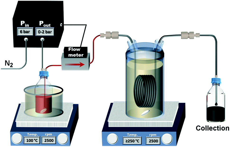Fig. 1 Schematic of the continuous thermal decomposition synthesis set-up.

Reactor operation. Initially, the precursor solution was preheated to 120 °C in a sealable flask for at least 30 min while purging with nitrogen using the pressure pump to i) remove water, ii) remove dissolved oxygen, and iii) completely dissolve the Fe(acac)₃ powder. The solution in the flask was then cooled to 100 °C under nitrogen. To initiate the continuous thermal decomposition synthesis, the pressure pump was connected to the flask inlet followed by a tubing immersed in the precursor solution at the bottom of the flask (which was initially used for nitrogen purging). First, the pressure in the flask was set to 400 mbar till the precursor solution passed the flow meter. Subsequently, the control mode was changed from pressure control (i.e., maintaining the pressure) to flow rate control (i.e., maintaining the set flow rate using feedback control of the pressure based on the flow rate measured). In order to avoid any sedimentation in the flow meter, it was heated to 50 °C using a customised heater covering the lower part of the flow meter containing the measurement capillary. Further details of the heater for the flow meter and the calibration of the latter are provided in ESI-2.1.† After the flow meter, the precursor solution passed the tubular reactor which was connected at its end with 1 m of PTFE tubing to guide the solution to the sample collection. During the synthesis minor gas formation was observed, i.e., bubbles exiting the reactor at a low volume fraction of ∼2% at temperatures close to room temperature. This was attributed to gaseous decomposition products of the Fe(acac)₃ such as acetone and CO₂.⁴⁴

It should be noted, that although the precursor solution was kept at 100 °C, its temperature dropped during transfer to the reactor through the PTFE tubing. Therefore, preliminary studies monitoring the pressure drop and changes in feed concentration over time were performed, which did not indicate any precipitation or accumulation in the tubing (see ESI-2.2†). In fact, the precursor solution remained stable, i.e., the solution remained clear without any signs of precipitation, even at room temperature. This was attributed to a complex formation of Fe(acac)₃ with oleylamine which agrees with the observed change of the UV-vis spectrum (see Fig. S7†).

Characterisation

Transmission electron microscopy (TEM). TEM studies were performed on a JEOL 1200 EX microscope (JEOL Ltd., Japan) with a 120 kV acceleration voltage. Samples were prepared by precipitation of the particles from the as-synthesised colloidal solutions with acetone, centrifugation at 17 000 rpm (BioFuge Statos, Thermo Scientific, US) for 5 min, and re-dispersion in hexane. A drop of the sample was then deposited onto carbon coated copper grids and the solvent was let to evaporate before TEM analysis. Particle diameters were obtained using ImageJ by manually drawing polygons around ca. 100 particles (depending on the image), and assigning the diameter of a circle with the same area.

Small-angle X-ray scattering (SAXS). SAXS curves were recorded using a Ganesha 300XL SAXS (SAXSLAB, Denmark) featuring a point X-ray source and a 2D detector. Synthesised IONP solutions were transferred into borosilicate glass capillary tubes with an inner diameter of 1 mm without any preceding cleaning step, and spectra were collected for at least 1 h. Details on the spectra analysis are provided in ESI-3.† It should be noted that there was no treatment of the IONP solutions, such as any washing or ultra-sonication step, before the measurement. All spectra were recorded within 24 h after synthesis.

UV-vis. UV-vis absorption spectra of IONPs and precursor solutions were recorded via a USB 2000+ spectrometer and a DT-Mini-2-GS light source (Ocean Optics Inc., USA). Based on initial studies dissolving Fe(acac)₃ in isopropyl alcohol (IPA) the maximum concentration to remain in the linear Beer–Lambert regime was estimated as 0.02 mg Fe(acac)₃ per ml IPA (see Fig. S6†). Therefore, absorption spectra were recorded for mixtures of 0.08 ml collected IONP solution diluted in 60 ml IPA (see Fig. S7†). The latter was favoured over 1-octadecene, since disposable polymethyl methacrylate cuvettes with a transmission down to ∼250 nm could be used. Although the strong absorbance of Fe(acac)₃ required large dilutions (60.08 ml/0.08 ml = 751) for quantification via UV-vis spectroscopy, the absorbance of IONPs and the used solvents became negligible at these dilutions. Therefore, UV-vis spectroscopy provided a convenient method to determine the precursor conversion, similar to the procedure used by Uson et al.⁴³ The conversion was determined from the ratio of the maximum absorbance of the precursor solution A_prec and the sampled IONP solution A_sample, as follows: conversion [%] = (1 − A_sample/A_prec) × 100. For the precursor and sampled IONP solution, the maximum absorption (of the only absorption peak between 250 and 700 nm) was between 310 and 315 nm, whereas the solutions of Fe(acac)₃ in IPA only showed three absorption peaks with a maximum absorption around 280 nm, see ESI-4.2.† This change in the absorption spectra was assigned to the formation of Fe(acac)₃ complexes, most likely with oleylamine, during the preheating step when preparing the precursor solution. Such a complex formation is also in line with the mentioned stability (against precipitation) of the precursor solution once preheated.

Results and discussion

Operation at 250 °C

The reactor was operated at varying flow rates, hence IONPs were synthesised at different mean residence times t_r. The initial flow rate was set to 1.7 ml min⁻¹ (t_r = 3.7 min) followed by 3.7 ml min⁻¹ (t_r = 1.7 min), 2.7 ml min⁻¹ (t_r = 2.3 min), the lowest flow rate of 0.7 ml min⁻¹ (t_r = 8.9 min), and finally, set back to 1.7 ml min⁻¹ to test for reproducibility. This sequence of flow rates was chosen to ensure that any correlation between the residence time and the synthesis products cannot be assigned to any other temporal characteristic of the reactor operation. Samples of the synthesised IONP solutions were collected after waiting for at least three times the mean residence corresponding to the set flow rate. The feedback-controlled pressure pump made it possible to monitor the pressure required to maintain the set flow rates, which provided additional insights. For example, a continuous increase in pressure when the flow rate remains unchanged would indicate fouling of the reactor wall. The pressure and flow rate profile during the operation at 250 °C show that the pressure remained fairly constant after a short transient phase following each change in flow rate (see Fig. 2).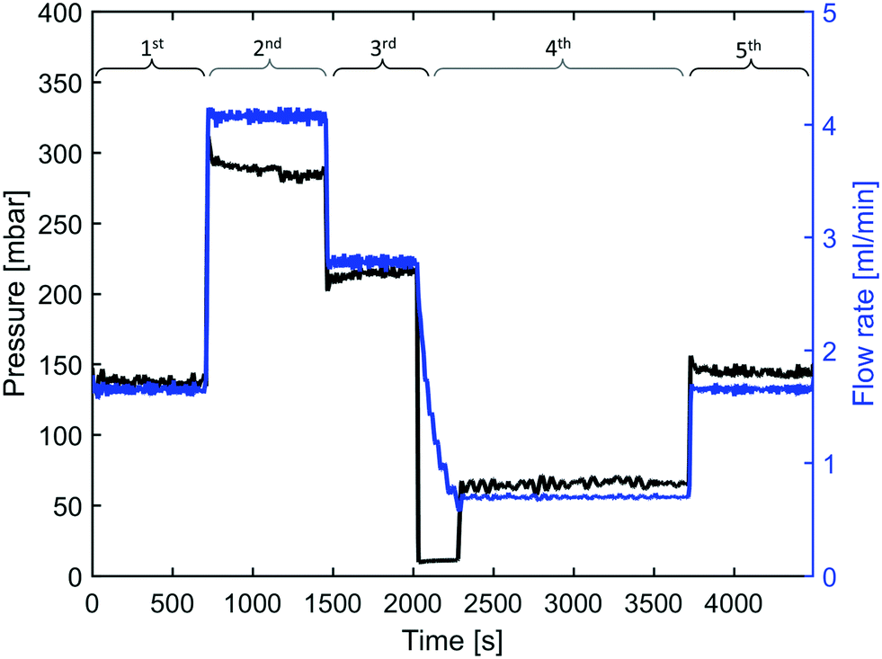

Fig. 2 Measured pressure and flow rate during the experiment at 250 °C for different flow rate/residence time settings. 1^st 1.7 ml min⁻¹, 2^nd 3.7 ml min⁻¹, 3^rd 2.7 ml min⁻¹, 4^th 0.7 ml min⁻¹, 5^th 1.7 ml min⁻¹.

The UV-vis spectra of the IONP solutions synthesised at 250 °C (diluted with IPA as described above) are shown in Fig. 3. The spectra show a decrease in the absorption assigned to the Fe(acac)₃ complex formed, with residence time, hence, an increase in the conversion. The samples collected for the 1^st and last (5^th) flow rate setting, i.e., with the same residence time of 3.7 min, had almost identical UV-vis spectra, indicating good reproducibility of the synthesis in this continuous reactor system.

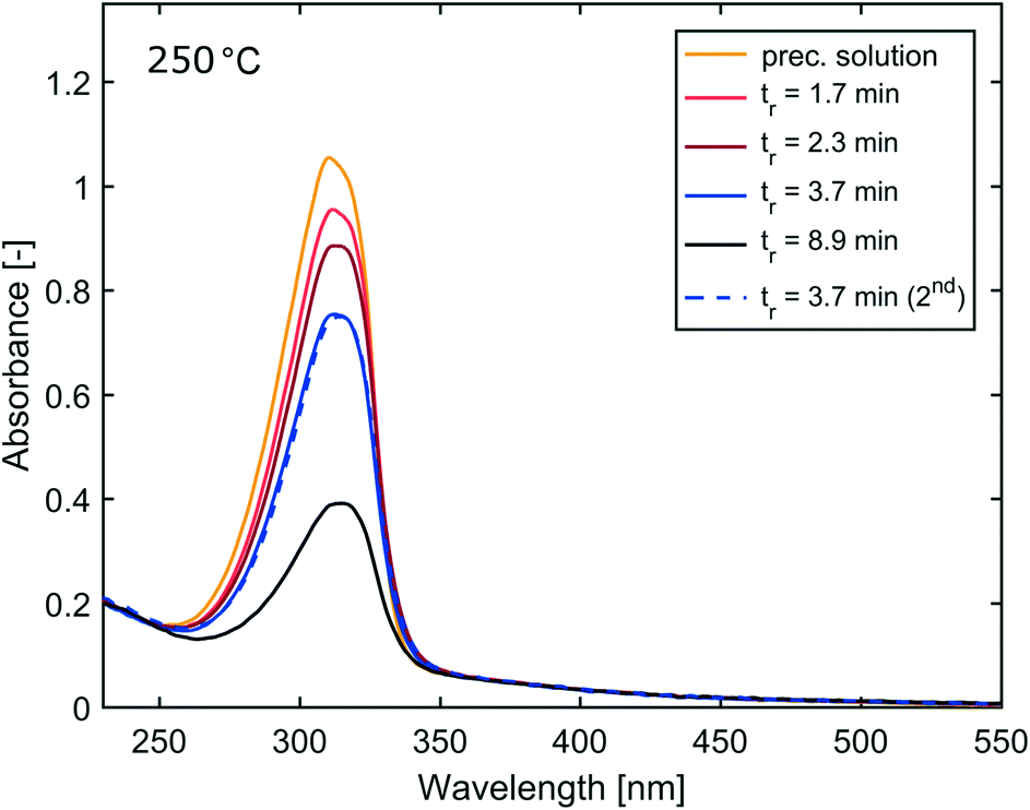Fig. 3 Absorption spectra of IONP solutions synthesised at 250 °C at different residence times.

The SAXS curves of the collected solutions are shown in Fig. 4. The intensities of the SAXS curves towards lower q-values are in line with the conversions obtained by UV-vis spectroscopy. The highest intensity, indicating more scattering bodies/NPs, was measured from solutions obtained from the longest residence time (8.9 min). The lowest intensity values were recorded for the two slowest flow rates (t_r = 1.7 min & 2.3 min). However, a direct correlation of intensities and number of nanoparticles is biased due to variations in the wall thicknesses of the single-use glass capillaries. Therefore, the intensities are not reported in absolute scale, (i.e., absorption per sample volume), which is possible only when using flow cells.⁴⁵

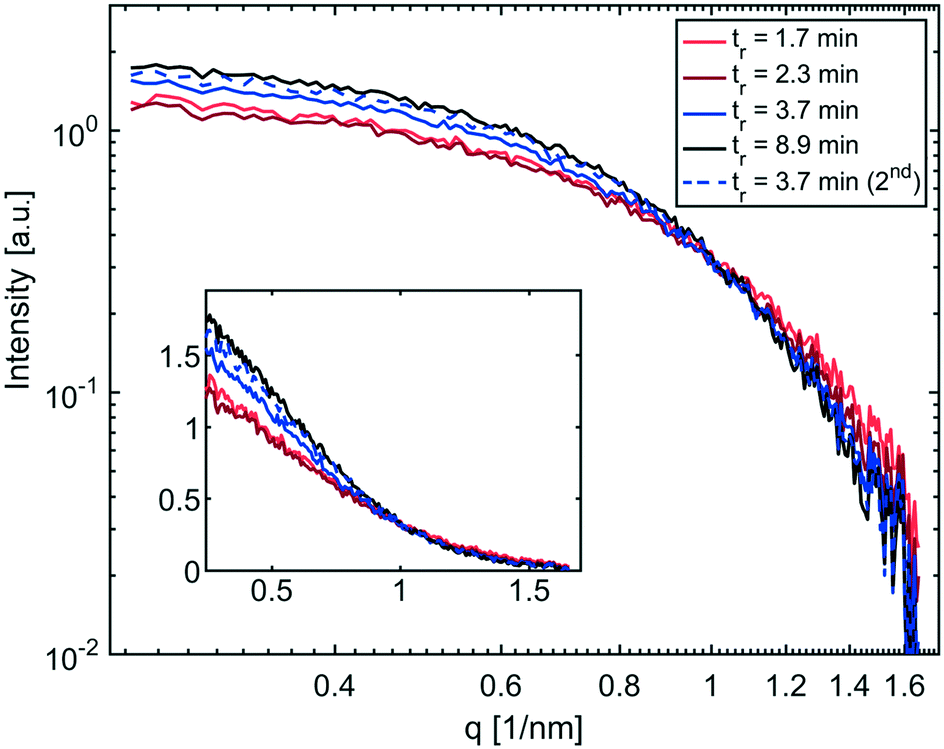Fig. 4 SAXS curves of IONP solutions synthesised at 250 °C and different residence times plotted using a logarithmic scale, and linear in the insert.

A summary of UV-vis and SAXS results for the synthesis at 250 °C is shown in Table 1, listing the conversion, the radius of gyration R_g (see eqn (S1) and (S2)†) and the resulting diameter assuming spherical particles D_sphere (see eqn (S3)†).

Table 1 Characterisation summary of samples synthesised at 250 °C and different residence times including the radius of gyration R_g, the diameter assuming spherical particles and precursor conversion

t r	R g (SAXS)	D sphere (SAXS)	Conversion (UV-vis)
1.7 min	2.15 nm	5.55 nm	9.4%
2.3 min	2.13 nm	5.50 nm	16.1%
3.7 min	2.25 nm	5.81 nm	29.0%
3.7 min (2^nd time)	2.23 nm	5.77 nm	30.3%
8.9 min	2.30 nm	5.93 nm	67.7%

---

Particle sizes obtained via SAXS are in good agreement with the TEM images shown in Fig. 5. Based on an unpaired t-test with a 5% significance level all diameters obtained by TEM analysis of samples obtained at 250 °C were shown to be significantly different, except the t_r = 2.3 min and t_r = 3.7 min sample. It should be mentioned that there are some variations in the sizes obtained by SAXS and TEM if particles are not highly monodisperse and isomorph. This is because of the poor statistical relevance of TEM⁴⁶ and the assumptions of the spherical particles for the calculation of D_sphere. Also, the scattered intensity scales with the sixth power of the particle diameter for SAXS, which is why the larger particles dominate the size analysis. The electron diffraction patterns (see Fig. S8)† confirm that the synthesised particles are of the inverse spinel structure, i.e., magnetite or maghemite.

Fig. 5 TEM images of IONPs synthesised at 250 °C and four different residence times (left: low magnification, scale bar = 100 nm); right: high magnification, scale bar = 20 nm, numbers are mean diameter and standard deviation. The corresponding histograms are shown in Fig. S9.†

Operation at 270 °C and 290 °C

Operation of the flow reactor at temperatures >250 °C worked likewise, except the additional purging of the heat transfer fluid with nitrogen gas as described in the Materials and methods section was employed. The UV-vis spectra of the IONP solutions synthesised at 270 °C and 290 °C show for both temperatures an increase in conversion with longer residence times (see Fig. 6). For 270 °C and 290 °C, the UV-vis spectra of IONP solutions produced at the beginning (1^st flow rate, 1.7 ml min⁻¹; t_r = 3.7 min) and end (5^th flow rate, 1.7 ml min⁻¹; t_r = 3.7 min for the 2^nd time) of the experiment are in very good agreement, indicating the reproducibility of synthesis conditions.

Fig. 6 Absorption spectra of IONP solutions synthesised at 270 °C (top) and 290 °C (bottom) and different residence times.

Comparing the conversion for equal residence times but different operating temperatures shows that higher conversions were achieved at higher temperatures. However, even at the maximum temperature of 290 °C, a 100% conversion, i.e., complete disappearance of the absorption peak assigned to the precursor complex, was not achieved (maximum conversion <70% based on UV-vis analysis). At 290 °C and a residence time of t_r = 3.7 min, the conversion was ∼56%, whereas t_r = 8.9 min gave a conversion of 70%, i.e., only 25% higher despite a 141% longer t_r.

For comparison, a batch study was performed heating 20 ml of the precursor solution to 270 °C in a 50 ml round bottom flask, (see ESI-6†) and showed that the conversion increased only marginally between 5 and 10 min after reaching 270 °C. This could be explained e.g. by the generation of iron complexes during the decomposition reaction that require temperatures >290 °C to decompose completely or decompose at a lower rate.

SAXS curves of solutions synthesised with the flow reactor at 270 °C and 290 °C are shown in Fig. 7. Similar to the synthesis performed at 250 °C, the SAXS curves show a trend towards higher intensities for solutions obtained at longer residence times, indicating more scattering bodies/NPs (in agreement with the UV-vis measurements). However, these intensities can be biased by varying capillary diameters as discussed above. A summary of UV-vis and SAXS studies for solutions synthesised at 270 °C and 290 °C is provided in Table 2.

Fig. 7 SAXS curves of IONP solutions synthesised at 270 °C (top) and 290 °C (bottom) and different residence times plotted using a logarithmic scale, and linear in the insert.

Table 2 Characterisation summary of samples synthesised at 270 °C and 290 °C and different residence times including the radius of gyration R_g, the diameter assuming spherical particles and precursor conversion

t r	R g (SAXS)	D sphere (SAXS)	Conversion (UV-vis)
270 °C
1.7 min	2.36 nm	6.09 nm	19.1%
2.3 min	2.37 nm	6.12 nm	31.8%
3.7 min	2.61 nm	6.74 nm	47.0%
3.7 min (2^nd time)	2.61 nm	6.74 nm	49.2%
8.9 min	2.61 nm	6.74 nm	69.2%
290 °C
1.7 min	2.14 nm	5.53 nm	36.2%
2.3 min	2.16 nm	5.58 nm	46.3%
3.7 min	2.27 nm	5.86 nm	56.3%
3.7 min (2^nd time)	2.20 nm	5.68 nm	55.8%
8.9 min	2.32 nm	5.99 nm	69.8%

---

TEM images of IONPs synthesised at the shortest and longest residence time are shown in Fig. 8. Again, the sizes obtained by TEM are in good agreement with the SAXS analysis, both showing particles of a similar size between 5 and 6 nm. Based on TEM analysis only the diameter of the sample synthesised at 270 °C and t_r = 8.9 differed significantly (from the other three samples) based on an unpaired t-test with a 5% significance level. Despite the similarity in size, the IONPs synthesised at 290 °C were more monodisperse compared to those obtained at 270 °C and 250 °C.

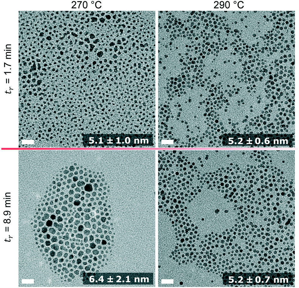Fig. 8 TEM images of IONPs synthesised at 270 °C (left column) and 290 °C (right column) at the minimum (first row) and maximum (second row) residence time. All scale bars represent 20 nm. The numbers are mean diameters and standard deviations. The corresponding histograms are shown in Fig. S10.†

For all flow experiments there was no evidence of fouling. Comparing the pressures during the flow experiments to maintain the set flow rate as recorded by the pressure pump showed no increase in pressure over time to maintain the set flow rate (Fig. 2 for 250 °C, Fig. S12† for 270 °C, Fig. S13† for 290 °C). Small changes in the pressure can originate from disturbances due to sample collection. Furthermore, cleaning studies (comparing the effluent of organic and HCl solutions) after each flow experiment did not reveal any signs of precursor accumulation or any particulate matter at the reactor wall (see ESI-2.3†).

Discussion of particle formation

The formation and growth of IONPs has been studied in detail for several thermal decomposition syntheses performed in batch. It is well understood that the interplay of nucleation- and (facet specific) growth rates, as well as the likelihood of aggregation determines the final IONP size distribution.^12,19,46 However, it is hard to compare flow with batch studies, as the rapid heating and cooling and the comparatively short residence times imply different process conditions. For example, the few studies of thermal decomposition syntheses in flow describe the synthesis of smaller (<7 nm) IONPs than obtained via batch procedures with comparable reagents.^41–43 This trend towards smaller particles in flow syntheses is not unexpected, as the rapid increase in temperature implies high thermal decomposition rates, and hence, higher nucleation rates leading to smaller particles.

The synthesis of <7 nm IONPs agrees well with our results, but we would like to discuss possible particle formation mechanisms briefly. It was shown via SAXS, UV-vis, and TEM studies that for all three reaction temperatures, the conversion increases with the residence time. However, when comparing the minimum residence time of 1.7 min and the maximum residence time of 8.9 min, the particle diameter increased by less than 1 nm (based on SAXS analysis). Also, the increase of the reaction temperature from 250 °C to 290 °C did not yield an increase in size of more than 1–2 nm, and a clear correlation between IONP size and the reaction temperature could not be observed. This conversion increase with residence time, without a significant change in particle diameter as observed for all reaction temperatures, indicates that the 5–7 nm IONPs did not form via a classical nucleation and growth mechanism, i.e., where nuclei ≪6 nm are formed initially and subsequently grow at a constant rate over time.

Three particle formation mechanisms that could explain the results are i) direct nucleation, ii) size focussing, or iii) growth via coalescence (see Fig. 9 for schematic representations).

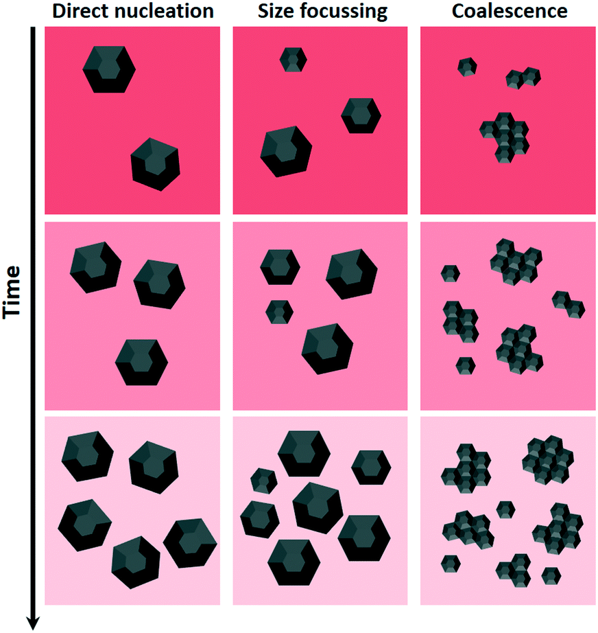Fig. 9 Schematic of the discussed growth mechanisms. The particle growth over time is represented vertically. The intensity of the background colour represents the amount of un-decomposed precursor.

i) The direct nucleation of 5–7 nm particles, in the absence of a considerable growth stage would explain the similar IONP sizes for all tested process conditions. However, the direct nucleation of IONPs of several nm seems highly unlikely. Unfortunately, information on the IONP nuclei sizes for thermal decomposition syntheses is scarce.^19,20 This is partly due to the experimental challenges associated with the analysis of temporal states of particles during high temperature syntheses. One exception is the recent study by Lassenberger et al. providing insights into the nucleation dynamics during thermal decomposition of iron pentacarbonyl (Fe(CO)₅) in the presence of oleic acid (OA) via in situ synchrotron SAXS and XRD studies.⁴⁶ The authors demonstrated that the formation of inorganic Fe-clusters was followed by burst nucleation and that the final particle size was dependent on the OA concentration. For low OA concentrations (molar ratio Fe(CO)₅/OA ≤0.84) the nucleation of 2–4 nm particles (i.e., the resolution limit of the applied methods) was followed by a short growth phase of only a few minutes yielding IONPs between 3 and 6 nm. Their results do not indicate the direct nucleation of >5 nm particles. However, it shows how burst nucleation (as expected for high thermal decomposition rates) can result in small IONPs as not enough precursor material is left after nucleation for significant growth.

ii) Size focusing due to non-linear growth, i.e., the growth rate G [nm s⁻¹] depends on the particle size (G = ΔD/dt = f(D)), with a slower growth for larger particles would be in line with our results. When considering the classical particle growth theory, this is the case for diffusion limited growth, where G ∝ 1/D,⁴⁷ with the highest growth rate just after nucleation. However, diffusion limited growth implies that neither the incorporation of thermal decomposition products into the IONP crystal lattice, nor the decomposition of precursor are the growth rate limiting step.

iii) Based on the non-spherical appearance of the synthesised IONPs (see TEM images in Fig. 5 and 8), growth via coalescence seems plausible. A higher probability for small particles to agglomerate (which is due to the high surface energy of small particles and its decrease with aggregation), would be consistent with the observed results. Also, TEM images do not show a significant fraction of <5 nm IONPs. When considering a growth mechanism involving coalescence, the stabilising effect of oleylamine needs to be considered too.⁴⁸ However, the limited knowledge on the dynamics of oleylamine binding to the IONP surfaces does not allow for a comprehensive discussion.

In general, the results do not allow for a distinction between the three suggested growth mechanisms and is likely that IONP growth occurred via a combination of different mechanisms (most likely including coalescence).

Cost analysis

With the aim to estimate the cost of IONPs production using the flow system described and for further comparison between batch and continuous systems, a cost analysis was carried out. The analysis refers to an 8 h shift, and takes into account the prices of chemicals, reactor equipment and labour necessary to produce IONPs in that specific time period. The costs of post-processing, e.g. separation and purification, were not considered.

For the flow reactor, the time for setting up the process was considered to be 1 h, which included solution preparation and preheating of the oil bath, and subsequent cleaning of the flow system. The remaining 7 h, were allocated only to the synthesis. The costs were calculated for an operation at 250 °C at a flow rate of 0.7 ml min⁻¹ (t_r = 8.9 min, 67.7% conversion) yielding a production volume of 294 ml (ca. 957 mg of IONPs, assuming IONPs are purely magnetite). For batch processing, a maximum daily production of 60 ml (corresponding to three 20 ml batch syntheses, see ESI-6†) with a conversion of 80% yielding 230 mg of IONPs was assumed. The comparison between the two systems is based on a daily production of 60 ml of IONP solution. Therefore, to be able to compare the systems, the production costs due to the synthesis in continuous flow were scaled to that volume. For both systems, the estimation of the operating hours has been kept conservative, to account of possible downtime. Details on the cost estimation are described below and in the ESI-8.†

Chemicals

The purchasing prices for the chemicals (see Table S2†) do not refer to the ones corresponding to the first part of this paper (see Table S1†), but to the cheapest prices found on several suppliers websites, and apply to volumes of materials that can be stored in a laboratory (maximum volume 25 l). Table S2† lists all the chemicals, including suppliers and prices, for the reactions and the cleaning and Tables S3 and S4† show the breakdown of the costs for chemicals for the production in batch and flow.

Reactor equipment

The prices of the reactor equipment include the glassware, the heat transfer fluid, tubing, the stirring hotplates and the flow meter. Information regarding the quantities and prices are reported in Table S5.† For each component of the continuous and batch system a lifetime was assumed based on a daily usage of 8 h for 248 working days per year. It was assumed that the flow reactor was operated 7 h per day and one year was assumed for the lifetime of the coated stainless steel tube. Tables S6 and S7† show the breakdown of the costs for reactor equipment for the production in batch and flow.

Energy

The energy demand was estimated based on the nominal power consumption of pumps and stirring hotplates, and their estimated operational time.

Labour

The labour cost was estimated assuming that all the operations are conducted in the UK by a laboratory technician, working 37 h per week. Using the sector data on the labour cost provided by the statistical office of the European Union an hourly rate of £30 was assumed.⁴⁹ It was further assumed that the flow and the batch system require one laboratory technician working 8 h per day (£240 per day). In the case of the batch system, the labour cost is equal to £4.1 per ml. In the case of flow system, the labour cost is lower: £0.83 per ml, due to the higher volume produced in one working day. ESI-8.3† provides the details of the cost estimation for energy consumption and labour.

The comparison of costs for batch and flow production based on our cost analysis is provided in Table 3. For both systems, labour was by far the most significant cost factor. The costs due to chemicals, energy, and reactor equipment were all comparatively small. Even for the flow system, the costs assigned to the reactor made up <5% of the total costs. For the flow system, the higher production volume that could be achieved per day (making the time-consuming heating and cooling steps redundant) was decisive for the significant reduction in costs compared to the batch system. However, this cost analysis compares two lab-scale systems. Production costs at industrial scales would depend on the scalability of both systems. For example, larger volumes can be used for a batch (assuming similar heating characteristics for reproducibility), whereas the flow system could be scaled up by increasing the tube size and flow rate, as well as by numbering up. All would reduce the production costs considerably by minimising labour costs. Therefore, this analysis should be considered as an approximate indication and not a universal prediction which system can perform thermal decomposition syntheses more economically.

Table 3 Comparison of costs for batch (conversion 80%, see ESI-6†) and flow production (0.7 ml min⁻¹; conversion 67.7%)

	Costs batch system		Costs flow system
	60 ml IONP sol.	1 g IONPs	60 ml IONP sol.	1 g IONPs
Chemicals	£8	£36	£3	£17
Reactor equip.	£2	£9	£2	£10
Energy	£1	£2	£1	£2
Labour	£243	£1056	£50	£254
Total	£256	£1103	£56	£283

---

Conclusion

In this work we described a reactor capable of continuous IONP production by means of a high temperature (250–290 °C) synthesis using inexpensive chemicals. Due to rapid heating and cooling in the flow reactor, the synthesis time could be reduced to less than 10 min. The most monodisperse particles were synthesised at 290 °C, where also the maximum conversion was achieved.

Synthesised particles were in the range of 5–7 nm, independent of the reaction temperature and the residence time, whereas the conversion of the precursor was shown to be dependent on both. These results could not be explained via a classical nucleation and growth model, which is why three other particle formation mechanisms were discussed: 1) the direct nucleation of 5–7 nm particles, 2) size focusing due to non-linear growth and 3) growth via coalescence. Of these three mechanisms, a combination of 2 and 3 seems most plausible.

An analysis of IONP production costs for the presented continuous synthesis was provided and compared with the costs of a batch system. This cost analysis showed that a continuous reactor for a high temperature synthesis has the potential to reduce the production cost. Labour was shown to be the dominant expense for both systems, followed by chemicals, reactor equipment, and energy. This reduction in labour has the potential to produce “more in less time” utilising a continuous flow reactor, since heating and cooling stages, as required for batch production, become redundant. A prediction of a possible cost reduction at industrial scale is challenging but our analysis for lab-scale systems indicate that continuous high temperature syntheses have the potential to reduce production costs.

A continuous production system can only be more cost efficient when long operation times are feasible. This requires a robust continuous process without significant fouling or even reactor plugging. The pressure recordings during the continuous synthesis, as well as the fouling studies performed subsequent to the experiments, showed no sign of fouling or accumulation of precursor material or other residuals at the wall, demonstrating the suitability of the reactor for long term operation and large scale production.

It should also be highlighted that, although the synthesis was developed at lab-scale, production volumes of ∼0.5 l d⁻¹ were possible with well controlled process conditions such as temperature profile and residence time. This guarantees identical process histories for the NPs produced. Consequently, the production of larger quantities, e.g. several litres per week, is possible by long term operation. This can make scale-up studies to achieve similar process conditions in larger reactors, which is still the common procedure for batch production, redundant.

Author contributions

The manuscript was written through contributions of all authors. All authors have given approval to the final version of the manuscript.

Conflicts of interest

There are no conflicts of interest to declare.

Acknowledgements

MOB, APL, MP, NTKT, and AG would like to thank EPSRC for funding (grant EP/M015157/1). NTKT thanks AOARD (FA2386-17-1-4042 award). SF thanks UCL-JAIST for funding his PhD studentship.

References

1. N. T. K. Thanh, Clinical Applications of Magnetic Nanoparticles: Design to Diagnosis Manufacturing to Medicine, CRC Press Taylor & Francis Group, London, 2018.
2. M. Mahmoudi and S. Laurent, Iron Oxide Nanoparticles for Biomedical Applications : Synthesis, Functionalization and Application, Elsevier, Amsterdam, 1st edn, 2017.
3. J. Xie, R. Jin, A. Li, Y. Bi, Q. Ruan, Y. Deng, Y. Zhang, S. Yao, G. Sankar, D. Ma and J. Tang, Nat. Catal., 2018, 1, 889–896.
4. S. Rajput, C. U. Pittman and D. Mohan, J. Colloid Interface Sci., 2016, 468, 334–346.
5. G. Cotin, S. Piant, D. Mertz, D. Felder-Flesch and S. Begin-Colin, Iron Oxide Nanoparticles for Biomedical Applications, Elsevier, Strasbourg, 2018, pp. 43–88.
6. S. Laurent, D. Forge, M. Port, A. Roch, C. Robic, L. Vander Elst and R. N. Muller, Chem. Rev., 2008, 108, 2064–2110.
7. R. Hachani, M. Lowdell, M. Birchall, A. Hervault, D. Mertz, S. Begin-Colin and N. T. K. Thanh, Nanoscale, 2016, 8, 3278–3287.
8. Y. Bao, J. A. Sherwood and Z. Sun, J. Mater. Chem. C, 2018, 6, 1280–1290.
9. R. Hudson, Y. Feng, R. S. Varma and A. Moores, Green Chem., 2014, 16, 4493–4505.
10. Z. B. Shifrina and L. M. Bronstein, Front. Chem., 2018, 6, 1–6.
11. D. Ling, N. Lee and T. Hyeon, Acc. Chem. Res., 2015, 48, 1276–1285.
12. M. Unni, A. M. Uhl, S. Savliwala, B. H. Savitzky, R. Dhavalikar, N. Garraud, D. P. Arnold, L. F. Kourkoutis, J. S. Andrew and C. Rinaldi, ACS Nano, 2017, 11, 2284–2303.
13. A. K. Gupta and M. Gupta, Biomaterials, 2005, 26, 3995–4021.
14. A. P. LaGrow, M. O. Besenhard, A. Hodzic, A. Sergides, L. K. Bogart, A. Gavriilidis and N. T. K. Thanh, Nanoscale, 2019, 11, 6620–6628.
15. T. Hyeon, S. S. Lee, J. Park, Y. Chung and H. B. Na, J. Am. Chem. Soc., 2001, 123, 12798–12801.
16. J. Park, K. An, Y. Hwang, J.-G. Park, H.-J. Noh, J.-Y. Kim, J.-H. Park, N.-M. Hwang and T. Hyeon, Nat. Mater., 2004, 3, 891–895.
17. B. H. Kim, N. Lee, H. Kim, K. An, Y. Il Park, Y. Choi, K. Shin, Y. Lee, S. G. Kwon, H. Bin Na, J.-G. Park, T.-Y. Ahn, Y.-W. Kim, W. K. Moon, S. H. Choi and T. Hyeon, J. Am. Chem. Soc., 2011, 133, 12624–12631.
18. S. Sun and H. Zeng, J. Am. Chem. Soc., 2002, 124, 8204–8205.
19. S. G. Kwon, Y. Piao, J. Park, S. Angappane, Y. Jo, N.-M. Hwang, J.-G. Park and T. Hyeon, J. Am. Chem. Soc., 2007, 129, 12571–12584.
20. S. G. Kwon and T. Hyeon, Acc. Chem. Res., 2008, 41, 1696–1709.
21. A. Shavel and L. M. Liz-Marzán, Phys. Chem. Chem. Phys., 2009, 11, 3762.
22. P. Guardia, J. Pérez-Juste, A. Labarta, X. Batlle and L. M. Liz-Marzán, Chem. Commun., 2010, 46, 6108.
23. J. Van Embden, A. S. R. Chesman and J. J. Jasieniak, Chem. Mater., 2015, 27, 2246–2285.
24. A. Ali, H. Zafar, M. Zia, I. Ul Haq, A. R. Phull, J. S. Ali and A. Hussain, Nanotechnol., Sci. Appl., 2016, 9, 49–67.
25. C. Buzea, I. I. Pacheco and K. Robbie, Biointerphases, 2007, 2, 18–69.
26. V. S. Cabeza, in Advances in Microfluidics - New Applications in Biology, Energy, and Materials Sciences, InTech, London, 2016.
27. J.-M. Lim, A. Swami, L. M. Gilson, S. Chopra, S. Choi, J. Wu, R. Langer, R. Karnik and O. C. Farokhzad, ACS Nano, 2014, 8, 6056–6065.
28. J. H. Bannock, S. H. Krishnadasan, M. Heeney and J. C. De Mello, Mater. Horiz., 2014, 1, 373–378.
29. H. Yang, W. Luan, S. Tu and Z. M. Wang, Cryst. Growth Des., 2009, 9, 1569–1574.
30. A. M. Nightingale, S. H. Krishnadasan, D. Berhanu, X. Niu, C. Drury, R. McIntyre, E. Valsami-Jones and J. C. De Mello, Lab Chip, 2011, 11, 1221–1227.
31. M. Nishioka, M. Miyakawa, H. Kataoka, H. Koda, K. Sato and T. M. Suzuki, Nanoscale, 2011, 3, 2621.
32. X. Z. Lin, A. D. Terepka and H. Yang, Nano Lett., 2004, 4, 2227–2232.
33. H. Tang, Y. He, B. Li, J. Jung, C. Zhang, X. Liu and Z. Lin, Nanoscale, 2015, 7, 9731–9737.
34. A. Adamo, R. L. Beingessner, M. Behnam, J. Chen, T. F. Jamison, K. F. Jensen, J.-C. M. Monbaliu, A. S. Myerson, E. M. Revalor, D. R. Snead, T. Stelzer, N. Weeranoppanant, S. Y. Wong and P. Zhang, Science, 2016, 352, 61–67.
35. A. Adeyemi, J. Bergman, J. Brånalt, J. Sävmarker and M. Larhed, Org. Process Res. Dev., 2017, 21, 947–955.
36. M. Mirhosseini Moghaddam, M. Baghbanzadeh, A. Sadeghpour, O. Glatter and C. O. Kappe, Chem. – Eur. J., 2013, 19, 11629–11636.
37. A. P. LaGrow, T. M. D. Besong, N. M. AlYami, K. Katsiev, D. H. Anjum, A. Abdelkader, P. M. F. J. Costa, V. M. Burlakov, A. Goriely and O. M. Bakr, Chem. Commun., 2017, 53, 2495–2498.
38. M. S. Naughton, V. Kumar, Y. Bonita, K. Deshpande and P. J. A. Kenis, Nanoscale, 2015, 7, 15895–15903.
39. B. K. H. Yen, N. E. Stott, K. F. Jensen and M. G. Bawendi, Adv. Mater., 2003, 15, 1858–1862.
40. S. Marre, J. Baek, J. Park, M. G. Bawendi and K. F. Jensen, J. Assoc. Lab. Autom., 2009, 14, 367–373.
41. M. Jiao, J. Zeng, L. Jing, C. Liu and M. Gao, Chem. Mater., 2015, 27, 1299–1305.
42. W. Glasgow, B. Fellows, B. Qi, T. Darroudi, C. Kitchens, L. Ye, T. M. Crawford and O. T. Mefford, Particuology, 2016, 26, 47–53.
43. L. Uson, M. Arruebo, V. Sebastian and J. Santamaria, Chem. Eng. J., 2018, 340, 66–72.
44. J. Von Hoene, R. G. Charles and W. M. Hickam, J. Phys. Chem., 1958, 62, 1098–1101.
45. J. Maes, N. Castro, K. De Nolf, W. Walravens, B. Abécassis and Z. Hens, Chem. Mater., 2018, 30, 3952–3962.
46. A. Lassenberger, T. A. Grünewald, P. D. J. van Oostrum, H. Rennhofer, H. Amenitsch, R. Zirbs, H. C. Lichtenegger and E. Reimhult, Chem. Mater., 2017, 29, 4511–4522.
47. N. T. K. Thanh, N. Maclean and S. Mahiddine, Chem. Rev., 2014, 114, 7610–7630.
48. S. Mourdikoudis and L. M. Liz-Marzán, Chem. Mater., 2013, 25, 1465–1476.
49. Eurostat, Estimated hourly labour costs, 2017.

---

Footnote

† Electronic supplementary information (ESI) available: Additional experiments, and additional details of the set-up and methods used are provided in the ESI. See DOI: 10.1039/d0re00078g

---