
 Open Access Article
 This Open Access Article is licensed under a
 Creative Commons Attribution 3.0 Unported Licence
A tutored discourse on microcontrollers, single board computers and their applications to monitor and control chemical reactions†
Daniel E.
Fitzpatrick
 a,
Matthew
O'Brien
b and
Steven V.
Ley
*a
a,
Matthew
O'Brien
b and
Steven V.
Ley
*a
aDepartment of Chemistry, University of Cambridge, Lensfield Road, Cambridge CB2 1EW, UK. E-mail: svl1000@cam.ac.uk
bDepartment of Chemistry, Keele University, Staffordshire ST5 5BG, UK
First published on 6th January 2020
Abstract
This Tutored Discourse constitutes a preliminary exposure on how synthesis chemists can engage positively with inexpensive, low-power microcontrollers to aid control, monitoring and optimisation of chemical reactions. The acquired skillset adds a new aspect to the toolbox of molecular construction, especially going forward in an ever-increasing digital machine-assisted world. It attempts to break down some of the barriers and myths to adoption of these techniques and to provide a basis for further innovation and discovery.
Introduction
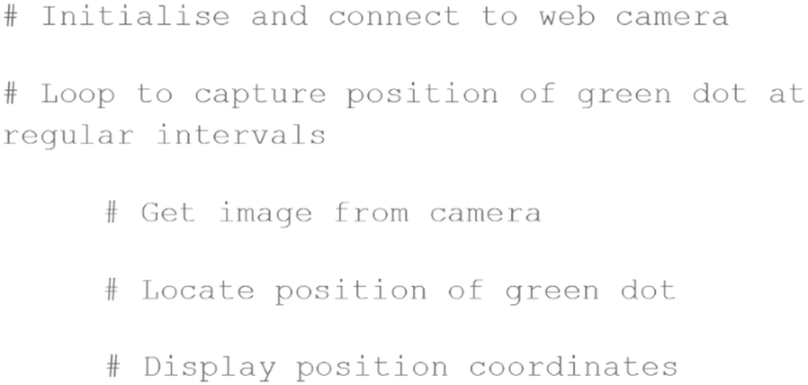
For many years now we have been advocating a machine-assisted approach to complex organic synthesis programmes.1,2 As part of this development, and the new world involving machine-to-machine learning and artificial intelligence (AI) algorithms,3 there has been a clear need to advance our knowledge of underpinning technologies. In particular, the role that inexpensive and commercially-available microcontrollers and single board computers can play in controlling and managing synthesis equipment over a wide range of applications and chemistries. While the benefits of using these devices can be truly game changing and create many synthesis opportunities,4 not the least of which is to facilitate maximising the human resource, synthesis chemists are mostly unfamiliar with these microcontroller units and particularly in writing appropriate operational code.In this Tutored Discourse we try to overcome some of the barriers to adoption of these methods by providing the beginning of a practical course to get started in the area. It is not our intention to go beyond a basic understanding at this stage; rather it is to provide the practising synthetic chemist with additional skillsets and language to better engage with engineers and those developing advanced machine learning techniques for future applications.
Applications
We initiated our own programme in computer control and microprocessors in 2012 when we had need to develop a new prototype magnetic field induced mixer device for flow chemistry.5 This unit was designed to afford excellent mechanical mixing within tubular flow reactors. In this work an ATmega 328P microcontroller was programmed with single C/C++ script commands to mechanically oscillate, in a linear fashion, a magnetic stirrer bar within a tubular flow mixer.In a second application (discussed in detail later) we devised a prototype continuous flow liquid–liquid extraction system,6 which has served us well in numerous examples. Here we used an inexpensive consumer webcam to observe and monitor the liquid–liquid interface enhanced by positioning a small green plastic float at the phase boundary. Using Python control scripts and several open source viewing packages we were able to provide appropriate feedback information and machine control to effect automated continuous extraction. The system could be extended to also achieve multiple stage liquid–liquid extraction of more complex and more polar reaction products.7
For a more comprehensive use of camera enabled techniques for organic synthesis, the reader is directed to a review of the area.8
Subsequently we harnessed the Raspberry Pi computer to monitor and control the automated multi-step flow preparation of piperazine-2-carboxamide (a component of Rifater used in the treatment of tuberculosis).9
During a further example for a flow-based synthesis of oxazolines and oxazoles, a software protocol written in Python was used to control a Raspberry Pi to drive reactor components, such as pumps and valves, in a pre-programmed sequence of timed actions.10
A complex systems approach towards intelligent self-controlling platforms for integrated continuous reaction sequences has been reported by our group.11 Here it is instructive to view how the different elements of chemistry, engineering and informatics12 are coordinated during a multistep preparation and downstream work-up of a key adamantane derivative needed for other work are managed.
For more general articles on the future of machine-based technologies we would recommend consulting the essay on The Internet of Chemical Things13 and an overarching review on enabling tools.14
Finally, in three further papers we describe particularly how web-based techniques operating devices through the internet15 and the cloud can enhance autonomous self-optimization and integration with batch processing,16 permitting remote control and access across the world, independently of time domains.17 Later in this paper we describe in more detail how these self-optimisation algorithms work and how they can be harnessed for a wide variety of applications.
We have also not been alone in developing these microprocessor-enhanced procedures and here highlight other work that further exemplifies the power of the methods.18,19
A Tutored Discourse
This article has been written to act as an introduction for chemists to the use of microcontrollers and computers for synthesis applications. It assumes no prior knowledge on the part of readers in the area of computer programming. Each of the following sections can be taken as separate lessons, which cover a wide base of material and include code examples. We have put together a list of materials and components (refer to appendix A) which can be purchased from commercial suppliers and which form the basis of examples in sections 1 through 4. The appendix also includes a glossary of terms used in various places throughout this article.The material covered has been put together from a hands-on workshop held at the University of Bielefeld as part of the ONE-FLOW research programme (Fig. 1).20
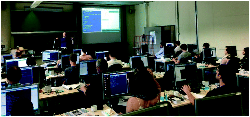 | ||
| Fig. 1 This Tutored Discourse is based on a workshop held at the University of Bielefeld (pictured above). | ||
Section 1. Introduction to microcontrollers, the Raspberry Pi and ESP32 board
What are microcontrollers?
The term microcontroller refers to a particular type of silicon chip which incorporates a microprocessor, memory and input/output peripherals together in a single integrated circuit. Since their emergence in the early 1970s, with devices like the Intel-4004 and the Texas Instruments TMS1000, microcontrollers have steadily grown in both capability and affordability. During this period, the development of modern non-volatile memory technologies (such as flash memory) has also dramatically increased their ease of use. A number of microcontroller families (including the AVR Atmega, STM32, PIC micro), have become very popular with hobbyists and educators. In particular, several microcontroller/programming systems have been specifically developed aimed at these markets, including the PICAXE, Basic Stamp and Arduino systems. These generally use a bootloader approach to program existing microcontrollers, allowing them to be reprogrammed with alternate language variants (for instance, PICAXE devices are PIC microcontrollers whose firmware has been modified to allow them to be programmed using a variant of BASIC).Microcontrollers can now generally be programmed from another computer (including the Raspberry Pi as described later in this section) simply by plugging in a suitable cable (e.g. USB) to perform a variety of functions depending on the capabilities of the circuit.
For example, most microcontrollers are able to measure changes in voltage applied to a pin which may, in a chemistry context, arise from changes in temperature (thermocouple) or acidity/alkalinity (pH probe) of a reaction medium. In addition to accepting input, microcontrollers are also usually capable of providing electronic output, from simply turning a voltage on or off, to the built-in use of common communication protocols (e.g. Serial/RS-232, SPI, I2C etc.).
While most modern computer systems run an operating system on top of which the user-facing software runs, the majority of microcontrollers are not sufficiently advanced or complex to support such operation. Instead, they are programmed directly, either using binary/assembly code or, far more commonly, binary code compiled from C-style languages such as C or C++. A variety of tools exist which allow the compilation (or conversion) of C code into a form suitable for running on the microcontroller, such as the Arduino IDE which we will use in sections 1 and 2.
The ESP32 board
The ESP32 series of microcontrollers (Fig. 2, right), developed by Espressif Systems in Shanghai, were released in 2016. The core architecture is based on a Tensilica/Xtensa dual-core LX6 32-bit microprocessor, running at 240 MHz. With built in Wi-Fi and Bluetooth, development boards based on these devices have become extremely popular, partly due to their low cost (ca. £7 per board) and impressive array of input/output channels. They can be programmed in C/C++ via a USB cable using the Espressif IDE.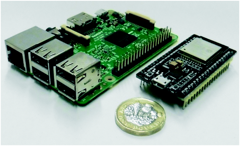 | ||
| Fig. 2 The Raspberry Pi computer (left) and ESP32 board (right), with a £1 coin for scale. | ||
Additionally, an ESP32 add-on for the Arduino IDE can be installed which allows them to be programmed using the Arduino variant of C/C++ (including the Arduino libraries) and this was the approach taken for the workshop. For several reasons, we used the Raspberry Pi single board computers to programme the ESP32 boards in the workshop. Although the Arduino IDE is available for the Raspberry Pi (Linux-ARM) system, a packaged ESP32 compiler toolchain for Linux-ARM systems was not officially available at the time of the workshop.
To get around this, we compiled the ESP32 toolchain for the Raspberry Pi using the Crosstool-NG system. It is not necessary to do this if the ESP32 is programmed on a regular Windows or Linux x86 system (for which toolchains were available). It should also be pointed out that all of the examples used in the workshop would also run on many other boards programmable using the Arduino Integrated Development Environment (IDE), a tool which enables users to write code, compile then write directly to connected Arduino boards.
The Raspberry Pi
Developed by the Raspberry-Pi Foundation to promote computer science education in schools, the Raspberry Pi single board computer (Fig. 2, left) was first released in 2012. Due to its low cost, small size, and range of input/output capabilities, it has rapidly become popular in the electronics and robotics hobby community and has been used in a number of scientific applications. Its central CPU is based on an ARM architecture and the latest version (RPi v4) has a quad core ARM Cortex A-72 processor running at 1.5 GHz. With versions having 1, 2 and 4 GB of RAM available, the Raspberry Pi is capable of being used as a general-purposed desktop computer. Although the officially released standard operating system is based on Linux (Debian), a range of operating systems (including Windows, FreeBSD and RISC OS) are available for it.The command line
Although the Windows operating system provides the user with a way of entering typed instructions (e.g. a command-prompt or powershell) this is, for most users, seldom used and the graphical user interface (GUI) is the principle method of interaction. However, in Linux-based operating systems (such as used on the Raspberry Pi) it is far more common to use the command line and, indeed, many fundamental tasks are more difficult to carry out without it. The workshop started with an explanation of how to open a ‘shell’ (the command line system) and with the basics of file system navigation (e.g. the cd, ls, mkdir, rm, mv commands). Specific details on the use of these core functions is beyond the scope of this Tutored Discourse, and so we direct interested readers to online resources for more information.21Writing a C script
Although the focus of the workshop was on programming the ESP32 in Arduino C/C++ and the Raspberry Pi in Python, it is useful for anybody interested in programming to understand how to compile C code on common architectures using the GNU C Compiler (GCC, a widely available open-source compiler). This began with the familiar ‘hello’ example, using Geany as the text editor to create the following code: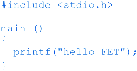
This simple program contains the basic components of C code. The ‘main’ function block (the only block in this case) is where execution starts. Blocks of code are contained within curly brackets {}. Each statement in a block (only one in this case) ends with a semi-colon. The #include statements allow various functions to be called. Here, the ‘printf’ function is contained in the ‘stdio.h’ header file. After saving (e.g. as ‘myfile.c’), this was compiled using GCC with:

To convert the input myfile.c file into the executable binary file myfile.out. This can then be run with:

Whilst this isn't particularly interesting (merely printing the text “hello FET” to the command line), it shows how straightforward the compilation process can be using the command line. More interestingly, a number of command-line tools allow the user to look inside the executable binary file:

Which shows the headers of the binary file, revealing that it is an elf (executable and linkable format) file, the standard binary executable format for Linux systems, as well as the architecture (ARM on the Raspberry Pi).

This command reveals the executable sections of the binary file, including the assembly language instructions (e.g. mov, pop etc.) which the C code is converted to.

The above can be used to reveal all the section headers.

And finally this command will open the binary file and show the actual zeros and ones (which ultimately correspond to turning voltages off or on) that make up the executable file.
While any detailed analysis of the binary files would be well beyond the scope of the workshop, this cursory inspection does reveal the link between the code files (which are generally the same for different operating systems and architectures) and the compiled executable binary files (which will be generally different for each type of computer architecture). It also makes clear the requirement for a suitable compiler for the desired target architecture. The vi command line text editor can also be used to view binary files if the ‘:%!xxd’ command is entered after opening the file to switch into binary mode.
In addition to these commands, the gcc compiler can also be used with the -S switch to create a text file (myfile.s) that contains assembly language instructions:

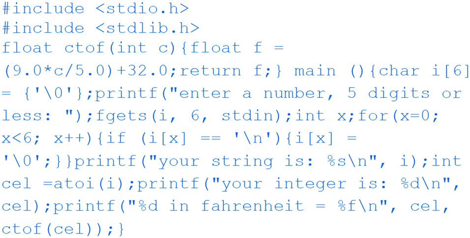
Before moving to the ESP32, a small number of basic C scripts were written and compiled/executed to introduce some basic components of the language. The final C code in this series, when executed, asks the user to enter a number and converts it from a Celsius temperature to a Fahrenheit temperature:
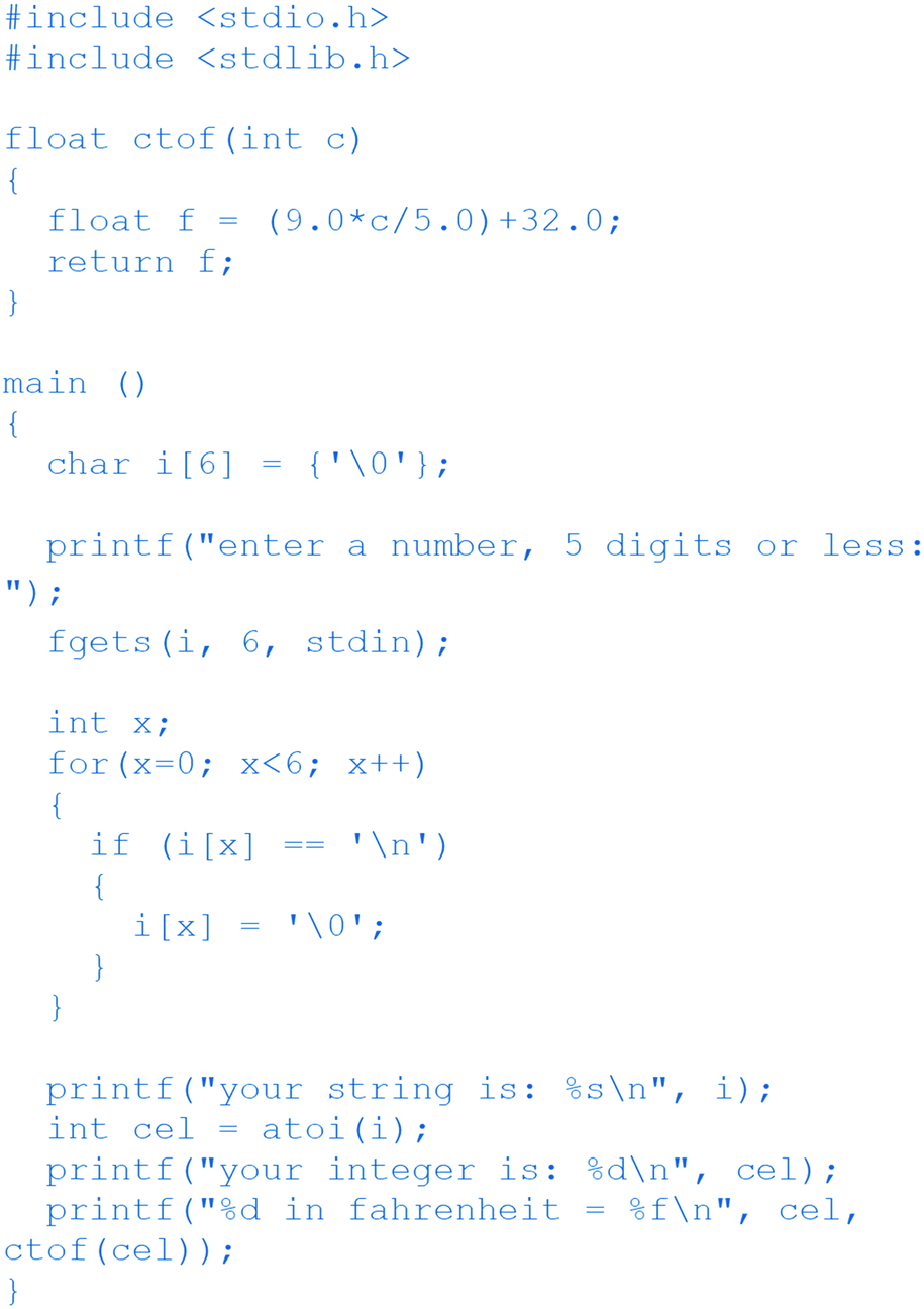
This simple program highlights a number of important aspects of the C programming language. Again, there is a main loop (where actual execution begins) as well as some #include statements which will ensure that the required functions are available. Before the main loop, a function ‘ctof’ is defined, which is later used within the main block.
When functions in C are defined, the variable name for the input (in this case ‘c’) as well as the datatype of the input (in this case ‘int’ for integer) must generally be defined within the brackets () after the function name. The datatype of the output (in this case ‘float’ for a floating-point number) must also be defined before the function name. This highlights the importance (and necessity) of memory space management when using C (each datatype uses a different amount of memory).
In the function ‘ctof’, a floating-point number f is declared which is the result of multiplying the input ‘c’ by 9.0, dividing by 5.0 and adding 32. The result is returned to the main loop. The function is called in the last line of the main loop: ‘ctof(cel)’ takes the value of the variable ‘cel’ and passes it to the ‘ctof’ function, which returns the corresponding output.
The first line of the main loop declares (and thus creates the required space in memory) a character array called ‘i’ which is 6 bytes long. This is essentially enough space to store 6 characters (letters or numbers). Each of these memory locations is then filled with the ‘\0’ character, which symbolised the end of the array. The ‘fgets’ line takes up to 6 characters of the text input by the user and places them in the character array i. The ‘for’ loop goes through each of these values and checks to see if they are equal to ‘\n’ (the return character) and, if so, replaces that character with the end-of-array character ‘\0’. In the character array, the value entered by the user is not in the correct form to undergo arithmetic operations, so is converted to an integer using the ‘atoi’ function, after which it can be passed to the ‘ctof’ function.
It is worth noting that with the C language, whitespace (e.g. spaces or blank lines in code, other than spaces between each command) or indentation (the starting position of each line) generally has no influence on the meaning of the code. For instance, the same script could equally be written as:
ESP32 scripts
The scripts for the ESP32 were written using the Arduino IDE on the Raspberry Pi. It is important to point out that many of the commands available in the Arduino IDE are non-standard commands in the C language, and won't be understood by a standard C compiler (such as GCC). These are part of the Arduino ‘libraries’, which are built in to the Arduino IDE system. More information about the libraries available can be found on the Arduino website.22The first script, shown below, blinks an LED connected to one of the pins of the board (in fact, it uses the built-in LED which is connected to pin 1). In this script, the pinMode and digitalWrite commands are Arduino specific terms.
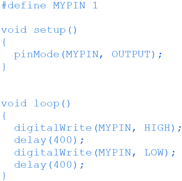
Unlike standard C scripts, which have a ‘main’ function/block, Arduino scripts (also known as sketches) have a ‘loop’ function/block, which repeats itself indefinitely. In addition, they can optionally also have a ‘setup’ block. The ‘setup’ block is where code execution begins. As the name suggests, this block executes once, when the program is run. Note that the name of each block/function is preceded by the word ‘void’. All functions in C must state the data type that will be returned by the function. If the function doesn't actually return any data (in other words it just executes code) then this is indicated by ‘void’. The setup function in this case tells the ESP32 to use pin number 1 as an output pin, meaning the program can turn it off or on (note: the #define line means that every instance of the word ‘MYPIN’ will be replaced by the number 1). In the ‘loop’ function, the voltage on the pin is either turned high or low, with a 400 millisecond delay in between each.
Generally speaking, Arduino C scripts are compiled using the button on the graphic user interface, although a command-line interface also exists. It is interesting to open the build folder for the Arduino IDE during compilation, as several files are created and destroyed, eventually leading to an executable binary file which is written to the ESP32 over the USB cable. It should be pointed out that compilation times for Arduino code on the Raspberry Pi can be very long. In order to save time during the workshop, precompiled binaries were also used. The binary files can also be opened using xxd and the other commands mentioned earlier.
Several aspects of Arduino C programming were demonstrated with a series of scripts and circuits, including one in which a potentiometer knob can be used to control the speed at which a motor turns. The circuit, which used an inexpensive 28BYJ-48 stepper motor (approx. £2 including driver board) had connections as shown in Fig. 3.
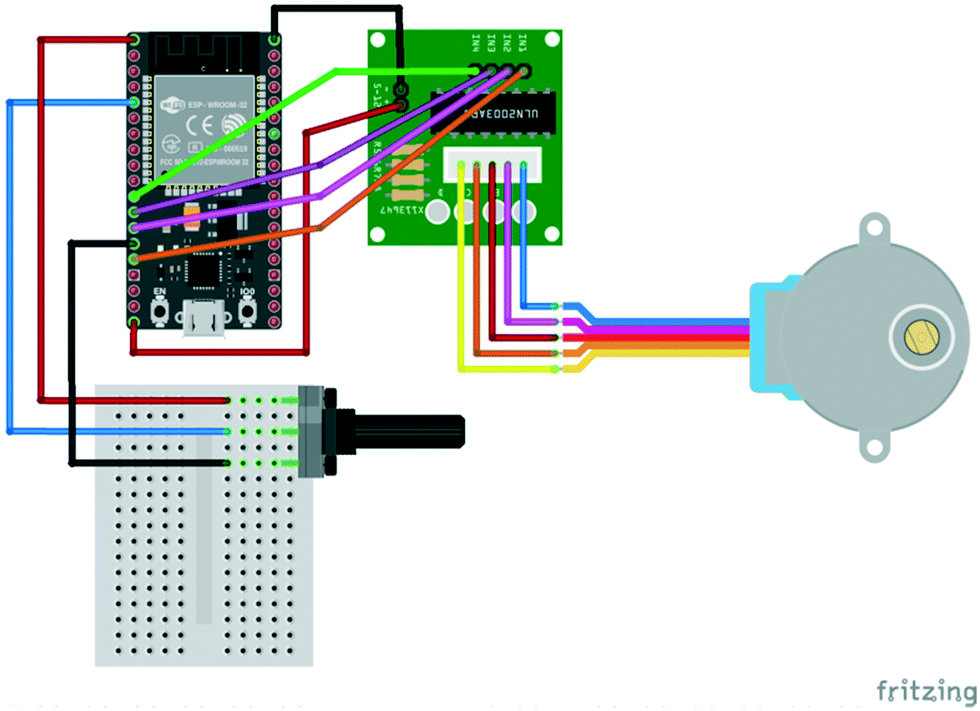 | ||
| Fig. 3 Wiring connections to drive a stepper motor using an ESP32 board and potentiometer. | ||
The corresponding script is shown below:

Before the ‘setup’ function, several variables are established, including those that hold the pin numbers which will be connected to the potentiometer and to the stepper motor driver board. The pin numbers for the stepper motor are placed into an integer array (called ‘pins’). The 8 × 4 array of boolean values (zeros or ones) called ‘stepseq’ is created. The motion of the stepper motor, as pins are turned on or off in this sequence should be possible to discern. The ‘ones’, which tend to move from left to right according to the sequence, correspond to magnets being activated. These magnets (or sets of magnets to be more precise) are arranged in sequences around the core of the stepper motor.
In the ‘setup’ function/block, the output pins are initialised and serial communication to the Raspberry Pi computer is setup (this allows text to be sent to the Raspberry Pi – or whichever computer the ESP32 was attached to – via the USB cable during execution). In the ‘loop’ function, two interleaved ‘for’ loops set the values of the output pins to match the values shown in the stepseq array. In the ‘outer’ loop, each time the sequence of output pin values changes, the voltage from the sensor pin (e.g. the one attached to the potentiometer, which can range continuously between 0 and 3.3 V) is read (using ‘analogueRead’ – another Arduino specific function) and this is converted to an integer value that ranges between 0 and 4096 (212 as the pin has a 12-bit analogue-to-digital converter). The delay function then uses this value to use up a certain amount of time until the next cycle of the outer loop. In this way, the potentiometer setting controls the speed at which the motor turns.
More example applications are included in the ESI.†
Section 2. Python and the Raspberry Pi
Introduction to Python
In the C programming language, memory has to be explicitly allocated for each data structure. For situations that require a more flexible approach (e.g. when the size of the data structure isn't known in advance), then dynamic memory allocation and reallocation is possible. However, this is one area where things can become quite technical for non-programmers.In recent years, a number of ‘high level’ programming languages have emerged that allow users to focus on the main desired functionality of the program without worrying too much about the detailed aspects of implementation. Python, developed by Guido van Rossum and first released in 1991, is one such language that has become extremely popular in a number of fields, including among the scientific community.
In very simple terms, it can be thought of as a programming system that sits on-top of lower level languages (such as C and Fortran). When scripts are run, they are compiled into something called ‘bytecode’, which is akin to a machine/assembly language for a virtual Python computer. This is then translated into the corresponding machine code for the particular hardware that the program is running on (this will generally be different on different architectures and/or operating systems). In this way, Python code should be transferrable from one machine to another. The language has been designed to be easy to learn and easy to use.
In many cases, the programmer does not need to worry about issues such as memory allocation. Generally speaking, Python is intended to be used on systems where significant memory is available, although variants (e.g. MicroPython and CircuitPython) are available for use on microcontrollers. Another significant feature of Python is the use of indentation level as a way to structure the code into blocks (c.f. the use of curly brackets in C, above). This generally makes code easier to read, although the indentation must be precise (each indentation level is either one tab space or four spaces).
Another significant difference between Python and C is the fact that Python has a REPL (read–evaluate–print–loop) shell available to it. This is somewhat similar to the command line shell in Linux, in that commands can be entered into the prompt. Data and variables are preserved throughout each shell session, allowing code to be run dynamically, one command at a time (e.g. without having to write a script and compile it first). This capability is not generally available using the C programming language. Although several IDEs and shells are available for Python development, the standard IDLE shell that comes with Python was used in the workshop. Most operating systems available for the Raspberry Pi have Python installed as standard.
Using Python with the Raspberry Pi
A simple REPL session was used to introduce several key features and data structures commonly encountered in Python (including variables, functions, and key data structures such as lists, strings, tuples and dictionaries). To provide some understanding of the link between Python as a high-level language and its low-level implementation in C, it is instructive to inspect the actual source code for various Python objects. For instance, the several pages of code for dictionary object (which can be downloaded from https://github.com/python/cpython/blob/master/Objects/dictobject.c) highlight the fact that Python handles quite a lot of detailed low-level implementation while providing a very simple and efficient interface.The first actual Python script written in the workshop simply turned a connected LED light on and off ten times in a row. The circuit is shown in Fig. 4 (only the green LED will be used, the other LEDs will be used in later scripts).
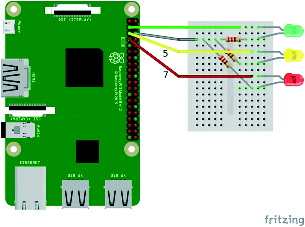 | ||
| Fig. 4 Wiring connections to power LEDs from a Raspberry Pi, using a Python script. | ||
The Python code is as follows:
The first line uses the ‘import’ command to import the RPi.GPIO module (which contains all the functionality required to control the GPIO input/output channels on the Raspberry Pi). The ‘as gpio’ means that we will henceforth call this ‘gpio’ instead of ‘RPi.GPIO’ (which simply makes it easier to write). The ‘import’ command is similar to the ‘#include’ statements in C. The second line also imports something from the ‘time’ module, but rather than importing the whole module, it just imports the ‘sleep’ function. The third line uses the ‘setmode’ function within the RPi.GPIO module (which we are calling ‘gpio’). The ‘dot’ notation seen here (in ‘gpio.setmode’) is common in Python and is a way to access the inner functions of modules or objects (so this accesses the ‘setmode’ function within ‘gpio’). The ‘gpio.BOARD’ sets up a particular numbering scheme for the GPIO input/output channels of the Rasperry Pi (there are two alternative numbering conventions). The fourth line sets up pin 3 as an output pin.
The main block in the code is a ‘for’ loop. This creates a variable called x, which will have values ranging from 0 to 9 (this is specified by ‘range(10)’). It then runs through the following block of code, once for each value of x in sequence. The ‘gpio.output(3, 1)’ line turns on pin 3 and the ‘gpio.output(3, 0)’ line turns it off. In between each, the program sleeps (i.e. does absolutely nothing) for 0.1 seconds. The indentation pattern for the ‘for’ loop is quite straightforward. Every line in the block is indented by one position exactly.
In a subsequent script, the user is asked to enter a command, and if either ‘green’, ‘red’ or ‘yellow’ are entered, the corresponding LED lights up. By placing this inside a ‘while True’ loop, the user will keep being asked to enter another colour once the blinking sequence has finished:

In this case, the code for the turning on and off of the LED pin is placed inside a function (called ‘blink’). Functions in Python are defined with the ‘def’ keyword, followed by the name of the function and also a variable name (or names) for input that will be provided to the function. Here, the letter ‘n’ is used. In Python, ‘while (statement)’ loops repeatedly run until the statement that follows them stops being true. By using ‘While True’, this loop will repeat forever, as the ‘True’ keyword will always be true. It is important to include some way to break out of the loop. The x = input (“enter colour:”) line asks the user for a colour and places the input word into a variable called x.
Notice that, in Python, a program does not need to specify the data type when a variable is created/declared. The ‘ledpins’ is a dictionary object. The ‘if x in ledpins’, looks to see if the word in x is actually in the dictionary, and if it is, send the corresponding number (e.g. 3 for green, 5 for yellow, 7 for red) to the blink function (which will then use this number in place of n). If the ‘if’ statement is not true (if the word entered is not in the ledpins dictionary), the else statement will execute (telling the user to enter one of the colours). If the user enters ‘quit’, the break command will cause the program to exit the loop. Note the nested indentation. For instance, the ‘if x in ledpins:’ line is indented relative to the ‘while True’ line, indicating that it is part of the ‘while True’ code block. The ‘blink (ledpins[x])’ line is further indented one position relative to the ‘while True’ line, thereby signifying that it is part of the ‘if x in ledpins’ code block.
An obvious limitation to the functionality of this code is the inability to have the blink function operate with different LEDs at the same time. In many situations, for all but the most simple of systems, it will be necessary to have the program doing several tasks simultaneously. One way to do this in Python is to use threading. Rather than have a single ‘thread’ of execution, we can have several ‘threads’ that run concurrently. The following code creates a new thread each time the user enters a colour. That thread then runs independently and execution passes straight back to the main loop, so the user can enter colours before waiting for existing commands to complete:
As can be seen, it is very similar to the previous script, except the simple call to the blink function has been change to the following two lines:

The ‘thread1 =’ line creates a thread object (called ‘thread1’). The ‘target = blink’ statement in the following brackets indicates that it is the ‘blink’ function that should be run in the thread. The ‘args = ledpins[x]’ statement tells Python that we want the value of ‘ledpins[x]’ (i.e. whatever number corresponds to the colour entered) to be passed into the blink function. The following line simply starts this thread running. When the blink function has finished (after the LED has blinked on and off ten times), the thread will effectively cease to operate. It does not matter that all threads will be given the name ‘thread1’ as they will all be independent of each other and we don't need to distinguish between them at any point.
Although this program does work, the operation might not be quite as expected. If the user keeps on entering ‘red’, before the previous ‘red’ blink function has finished, we will then have two different threads turning the red LED on and off, so the sequence will not be the same as before (i.e. turning on and off in the same sequence).
Perhaps a more desirable mode of operation would be for the user to enter commands (or more generally for the program to receive commands from some channel), and for these to be stored and run through with the original timing. In other words, if the user enters ‘red’ before a previous ‘red’ blinking sequence has finished, can we get the program to wait until the current ‘red’ blinking function has finished before starting the new one?
One way of doing this in Python is to use a queue object. This basically behaves as its name suggests. Items enter the queue at one end and leave at the other, in a first-in-first-out manner. We can have a queue for each type of LED (green, red and yellow) and place the corresponding commands in their respective queues. We can then have a thread for each colour that is responsible for checking for the presence of commands in its queue and, if one is present, activating the blink function for that LED. A simple version of such a program is shown below:
The script is quite similar to the previous one, except we now have three separate threads running – one for each colour, in addition to the main program thread (which runs the ‘while True’ loop that receives input from the user). We also have three queues that were created with the ‘redq = queue.Queue()’ line (and corresponding lines for yellow and green). The words ‘red’, ‘green’ or ‘yellow’ are placed in the relevant queue by the main ‘while True’ loop that gets user input. Each of the threads monitoring the queues (the redthread, greenthread and yellowthread) has a ‘while True’ loop that cycles through continuously checking to see if an item has been put into its related queue.
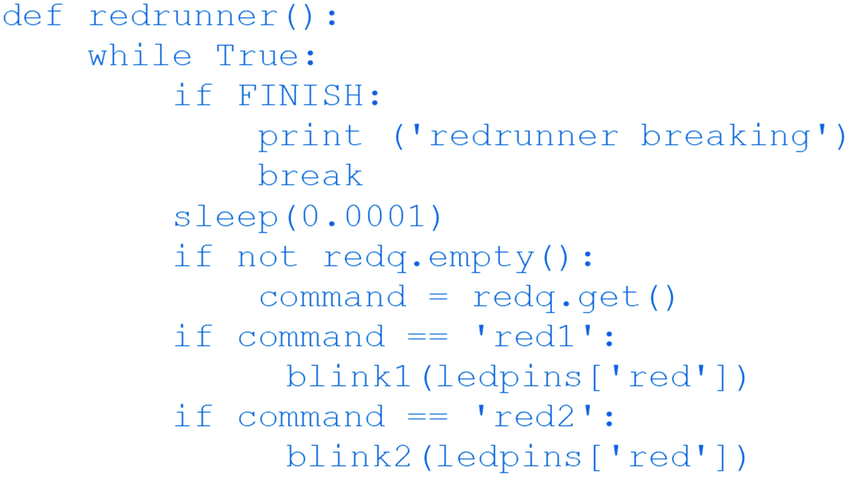
For instance, if the thread running the redrunner function sees something in the redq queue, it takes it out of the queue (so that the queue will have one less item in it), and then runs the blink function using the corresponding number from the ledpins dictionary. Note that this redrunner thread will then do nothing else until the blink function completes (as the blink function is not running in a separate thread). After the blink function finishes, execution will then return to the thread running the redrunner function and it will continue to repeat its continuous monitoring of the redq queue.
One line worth noting is ‘sleep(0.001)’ in the redrunner function. This prevents the computer using too much of its CPU/memory resources going through this ‘while True’ loop. If this line wasn't there, the program would still run but might well cause the computer to slow down as it could be running through the ‘while True’ loop as fast as possible (possibly billions of times per second). Checking the redq queue once every millisecond is fast enough.
Another feature of the redrunner, yellowrunner and greenrunner functions is that the ‘while True’ loop initially has an ‘if’ statement that checks to see if the FINISH variable is True. If this is so, the ‘break’ command causes execution to escape the ‘while True’ loop, essentially bringing the thread execution to an end. The FINISH variable is set to False at the start of the program. This kind of control variable is sometimes referred to as a ‘flag’ variable.
As written, this script will wait for any currently running ‘blink’ functions to complete before quitting. If more immediate quitting is required, then corresponding ‘if FINISH: break’ statements could be placed within the blink function itself. Also, whilst this script works as expected when executed from the command line on the Raspberry Pi, it sometimes doesn't cleanly exit if run from the IDLE shell. This can be solved by placing ‘redthread.join()’, ‘greenthread.join()’ and ‘yellowthread.join()’ statements before the final ‘break’ statement in the ‘if x==‘quit” block.
Note that, in this script, we are placing the ‘red’, ‘green’ and ‘yellow’ commands into the queues merely as placeholders. The program doesn't actually do anything in particular with these commands and we could actually put anything in the queue instead. However, in might often be the case that we want to place different commands into a queue and have the program act accordingly. For instance, if we had two different types of blink function, blink1 and blink2, and wanted to be able to run either, depending on the user input, we could use:
Of course, the section of code relevant to the user input would also have to be changed to accommodate this.
While these examples have been fairly simple, more complicated threading operations may be required, and this might involve creating new threads from within threads, which is perfectly possible. For instance, if we had created several functions called func1, func2 and func3 we could create a dictionary (called ‘funcs’ below) linking the words ‘func1’, ‘func2’ and ‘func3’ (or whatever words we wished) to the functions themselves:

The corresponding function code (e.g. for redrunner) would then look like:
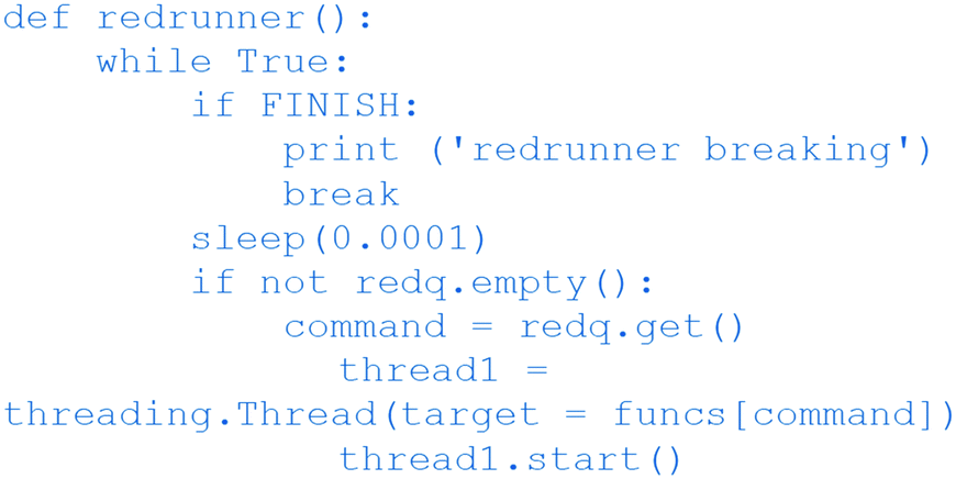
This then creates a new thread for each command placed in the queue, and the function running within each thread depends on the command itself. Note that, in this function as written, the threads will be created as soon as the command enters the corresponding queue (e.g. redq). If we want to wait for one threaded function to complete before we start the next one, we can add the following line just after the ‘thread1.start()’ line:

This essentially forces the redrunner function to wait until thread1 has done whatever it is supposed to do before continuing with its own execution.
Section 3. Applications to chemistry and machine vision
Automation and control for chemistry
The first two sections provide a general overview of how microcontrollers can be used to manipulate peripheral units, such as stepper motors and LEDs. These examples can be adapted to suit a chemical environment already; for example, a stepper motor could be used to change a valve position and a group of precise-wavelength LEDs could be used to irradiate a photo-catalysed reaction. In the following three sections, we will discuss how the material above can be applied in further experiment applications.There exist many examples in literature where control systems have been harnessed to automate synthetic procedures. As this area has been well-reviewed previously,1,2 we will highlight a few specific examples from our own research group here.
Recently we have reported the development of a reaction monitoring and control platform,15 which was used to automate a cycling catalytic process and conduct self-optimisation using both mass spectrometry and infrared spectrometry to determine performance of automatically-generated experiments (Fig. 5). More information about self-optimisation algorithms and how you can apply them to your own experiments is covered in Section 5.
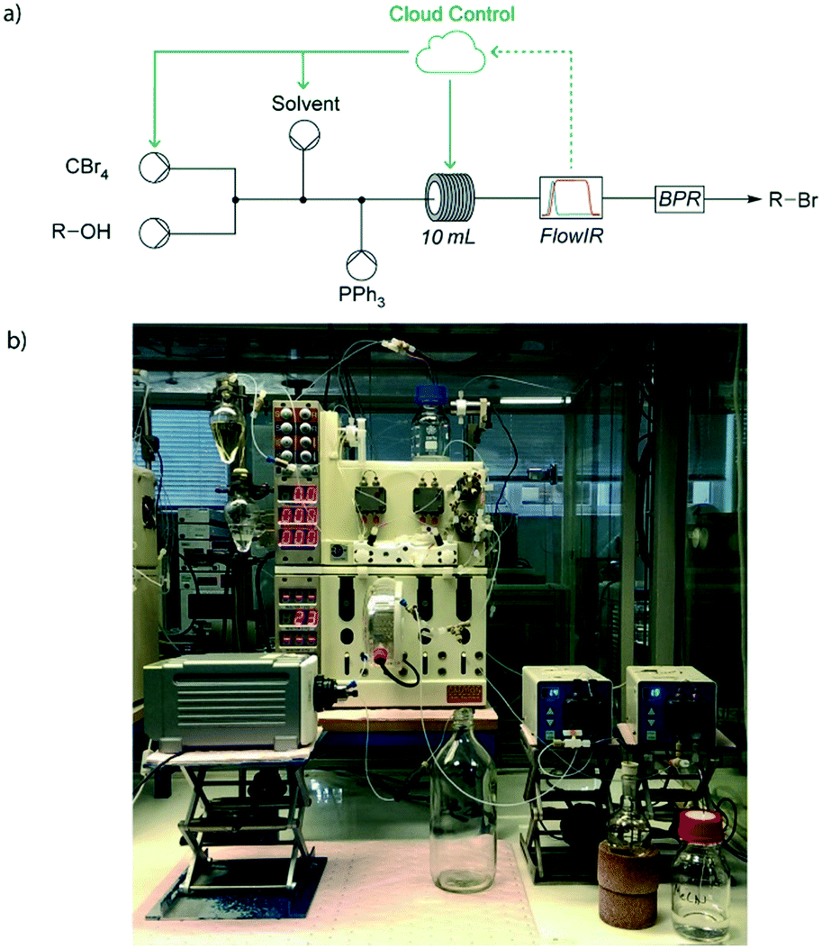 | ||
| Fig. 5 a) Feedback from an in-line IR detector was used to determine new experimental conditions, such as pump flow rates and reactor temperatures; b) photograph of the experimental set up for a five-dimensional self-optimisation of an Appel reaction. Adapted from ref. 15. | ||
The same system has been used to perform multi-step, telescoped reaction sequences where material from upstream reaction steps was directed to subsequent reactions without manual intervention or purification by operators.16 Inter-stage liquid–liquid extraction and solvent switching were also automated in this process, allowing batch and flow procedures to be integrated when producing 5-methyl-4-propylthiophene-2-carboxylic acid, a precursor to the anti-cancer drug candidate AZ82.
Both of these reports utilised machine vision for key elements of automation, as discussed in more later in this section. For the first, a Raspberry Pi and consumer webcam were linked to the control system to monitor the fluid level in a reagent reservoir. For the second, a webcam monitored the position of an interphase boundary in a continuous liquid–liquid extraction system.
Software for automation
The examples above utilised a software platform developed using a mixture of two programming languages; namely PHP (to more easily facilitate the web-based nature of the system) and Python (to integrate with reaction equipment). Section 4 covers networking and in particular how the Raspberry Pi can be connected to the internet in such a way as to enable remote control of your own equipment.It is worth noting, however, applications of automation do not exclusively use either PHP or Python. Indeed, there have been many reports of other packages being used to perform similar functions. One of the most popular has been LabVIEW, as discussed in a recent perspective,23 largely owing to its visual nature and resulting ease of use for researchers with limited programming experience.
Machine vision
By connecting a consumer grade webcam to computing devices, it is possible to give control software the ability to view chemical processes in a similar manner as a human operator. For example, the movement of reaction fronts can be observed24 and colour changes can be monitored.25 In 2013 we published a review covering a variety of applications of machine vision as applied to synthesis.8These applications primarily rely on the detection of boundaries within an image frame, such as that gathered in real-time by a web camera. For the examples described above, the position of a green plastic float was monitored via a relatively simple process where green-heavy pixels were identified and tracked. If the bulk of these pixels moved then appropriate control script decisions were made; when monitoring the fluid level in a reservoir (Fig. 6a) this might involve following a shutdown procedure if holdings of feedstock solutions were to deplete, or during an extraction the fluid flow drawn from a separating column (Fig. 6b) might be increased or decreased to maintain the position of the interphase boundary.
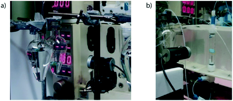 | ||
| Fig. 6 a) Inexpensive consumer-grade web cameras have been used to monitor fluid levels in reservoirs during experiment automation; b) similar technology has been used for continuous liquid–liquid separation. | ||
Raspberry Pi and Python for machine vision
Fortunately the heavy-lifting of image processing and analysis can be relegated to an open-source software package called OpenCV,26 and so adding support for machine vision to your own applications is relatively straightforward.Within Python, a wrapper library has been created which simplifies the use of OpenCV even further. Software libraries contain sections of pre-written code which perform common actions or define useful variables which can be used and referenced in your own code. In this case, SimpleCV condenses the steps needed to connect to your web camera and acquire an image into a few lines of code. It also contains functions to perform colour processing/analysis of images, as demonstrated in the example below.
Example
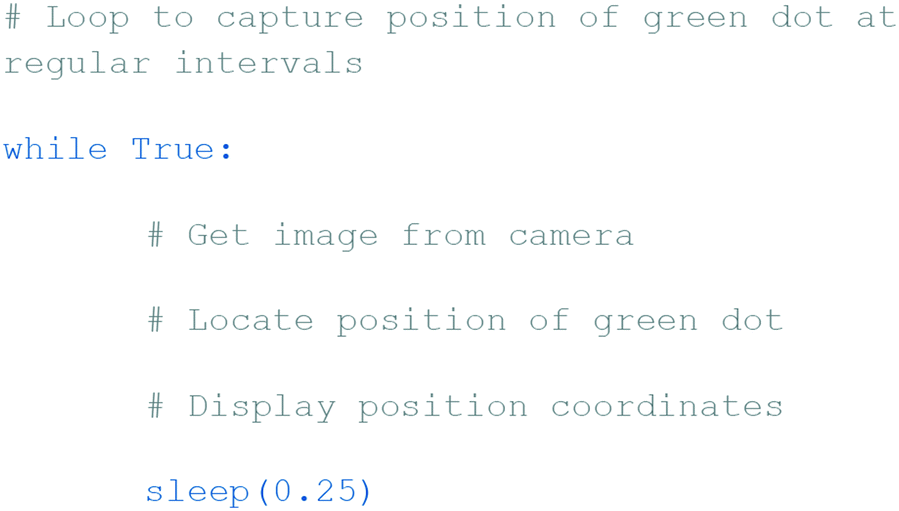
In this example, we will use a Raspberry Pi and consumer grade web camera to detect the position of a green dot on a printed sheet of paper (appendix B). We will be writing a Python script using SimpleCV to output the coordinates of the dot to a file on the Raspberry Pi. This exact process was followed in our own work where a green float was tracked (see above).Before we begin to write our application code, we first need to ensure that we have installed SimpleCV and any of its prerequisites to our Raspberry Pi. At the time of writing, this process is described on the SimpleCV website.27 We recommend that you browse to this website using your Raspberry Pi to download the tools required for your operating system and version of Python. After installing SimpleCV, select a directory on your desktop (or in whichever parent directory you wish) where a new script file can be created.
Pseudocode refers to an informal description of the actions/steps code should perform to achieve a desired outcome, designed primarily to be human-readable. It offers a high-level overview of the objectives of each segment of a script and can be used to great effect when planning your code. For this example, we've listed some pseudocode below which we will then expand with Python commands.
A loop block has been included above as the indented steps underneath need to be repeated at regular intervals to ensure that the position of the green dot is monitored over time, rather than captured just once when the script starts.
Let's start with the first line of pseudocode, which initialises and connects to the camera connected to the Raspberry Pi. The SimpleCV library simplifies greatly this process, handling all elements of hardware communication and driver response. Only a single line of code is required, after importing the SimpleCV library:
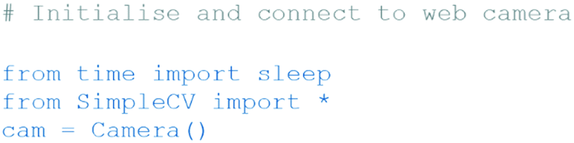
For the loop block, we'll create a very simple structure which will repeat itself constantly until the script is terminated. This can be done via the command line by pressing Ctrl + C when a script is running. The  command at the end of the looping block simply pauses the code cycle repeating by a quarter of a second, decreasing CPU load on the Pi.
Capturing an image from our web camera is the next step, and is achieved again using just a single line from the SimpleCV library. Here the image object is saved into a variable which we have called  .
.

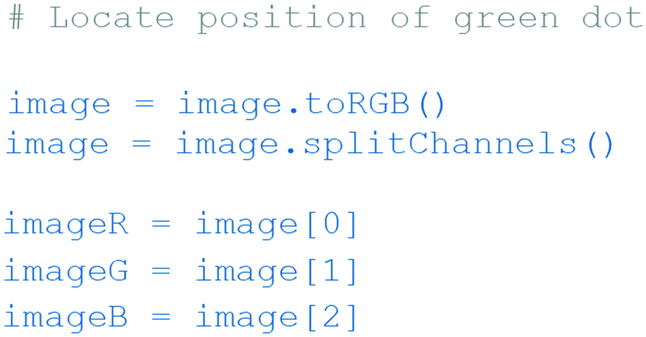
The next step, where the position of the green dot is determined, requires a few lines of code to achieve. One handy function available in SimpleCV allows us to separate the image object into a list containing three objects: the red, green and blue components of the original image, which we have assigned to their own variables in the code below. In Fig. 7a and b, the output for an example image is shown.
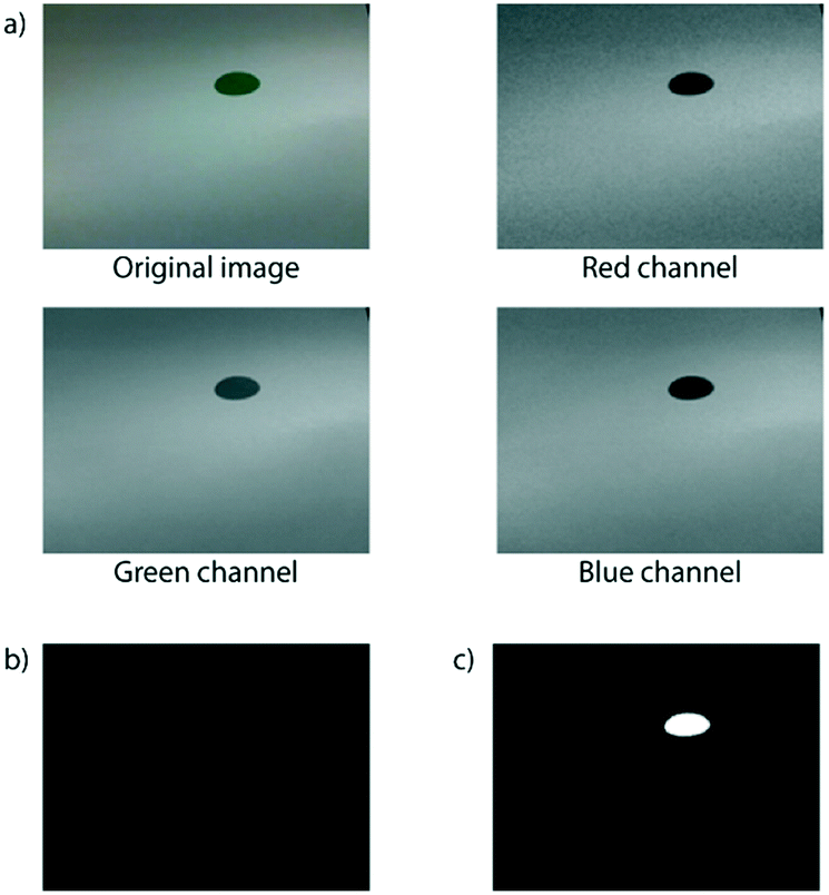 | ||
| Fig. 7 a) The original image captured by the web camera and processed images following separation of the red, green and blue channels of the original image; b) image output following the subtraction of the green channel from the blue channel; c) final output after the ‘binarize’ function, then inversion. | ||
The image objects above are not yet in the required form for us to reliably determine the position of the green dot. We first need to perform some more processing, again using functions built into the SimpleCV library. The first step is to subtract the blue channel from the green ( ), leaving us with an image showing where the green dot is on paper. Then the
  command will convert each pixel into either black or white depending on its original colour/greyscale value.
In order to prepare the black and white image object for the final command, where the position of the green dot is calculated, we first must invert the image using the  function. This will return an image object in the format (Fig. 7c) required for the
  function, which finds the position of any white spots on a black background in a Python list.

Finally, the last step in our pseudocode is to display the coordinates of the blob (or green dot) to the user. This can be achieved using the  command.
Section 4. Networking and remote control
Recently we reported an application of reaction control and self-optimisation which was spread across the world geographically.17 The equipment on which reactions were conducted and analytical data collected were located in our laboratories in Cambridge, UK, while the control server directing all experimentation was based in Tokyo, Japan. An operator was able to initiate and monitor reaction progress for all examples from Los Angeles, USA. Such an arrangement removed both time and space restrictions on experimentation, greatly enhancing our research regime.This programme could only be achieved by exploiting the ease of communication enabled by computer networking. In this example, the server communicated with equipment via TCP/IP and the operator interacted with the server also via TCP/IP (Fig. 8).
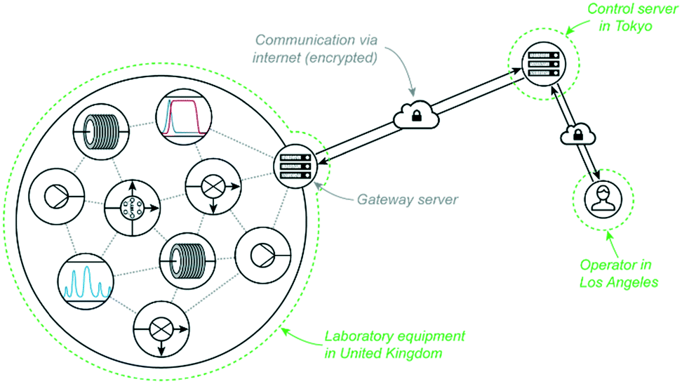 | ||
| Fig. 8 Global networking through the internet was exploited to perform rapid self-optimisation experiments for three API targets, allowing an operator in the United States to control equipment in the United Kingdom through servers in Japan.17 | ||
While the global networking of equipment in our report required a fairly complex set-up to facilitate communication (as detailed in the original paper), you can create a local network in your own laboratory without relying on any specialist knowledge. Indeed, simply connecting your Raspberry Pi by ethernet into a router will allow you to remotely access and control equipment, as detailed in the example below. This simple arrangement was exploited in a recent report where 24 individual pieces of equipment were controlled to enable semi-continuous separation of flow streams by supercritical fluid chromatography.28
When a new device is connected to a network, it is assigned an IP address automatically which is used to direct traffic accordingly. If your device is configured to act as a web server, it can respond to queries for information via standard HTTP (or HTTPS) ports (80 and 443 respectively). In other words, you can set up your Raspberry Pi to act as a server and then access information from it through an internet browser on another device on your network by entering in its IP address into the URL field. This process will be followed in this section's example to enable you to control a Vapourtec R2R4 from another device, such as your mobile phone or a tablet.
Cherry Py
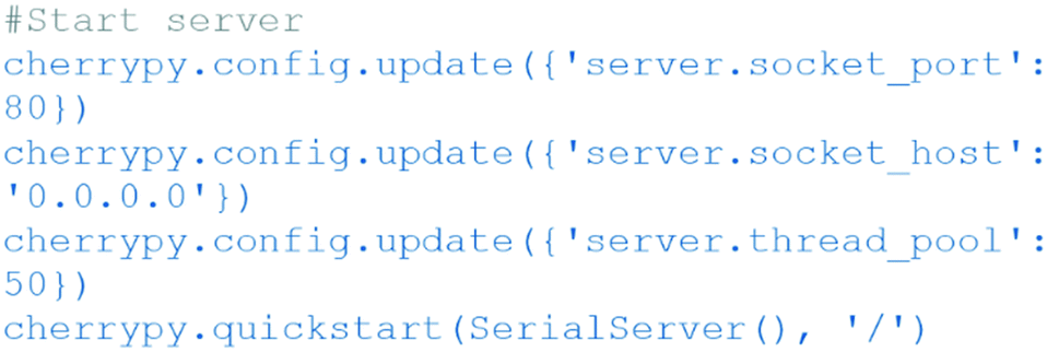
A Python library called CherryPy contains the functionality we require to set up the Raspberry Pi unit as a fully-functional web server. When a script which incorporates CherryPy is executed, a new process is created which listens for requests incoming to port 80 (the standard HTTP port) on the host device. The script can be configured to return information in a fully customisable manner, or process instructions as supplied in the URL (more detail about this is given in the example below).In a chemistry context, our group has used CherryPy with good effect to create remote equipment control stations (RS232) from a single Raspberry Pi (Fig. 9). Individual units have been used to control up to 24 pieces of laboratory equipment simultaneously. The full source code for the script in this case has been included in appendix C, which builds upon the example below.
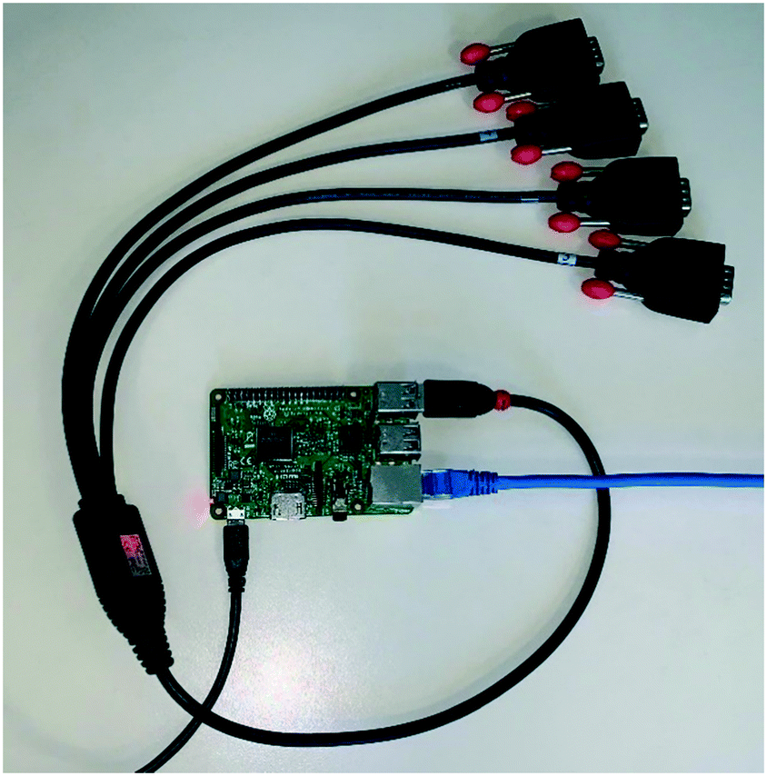 | ||
| Fig. 9 Photograph of an operational Raspberry Pi (version 3) web server configured to enable remote control of RS232-compatible laboratory equipment. | ||
In order to install CherryPy on your computer, we recommend following the instructions on the CherryPy website.29
Integrating laboratory equipment with an RS232 server
In this example we will write a script in Python that performs two key functions that are required to add RS232-compatible equipment to your network. The first command initiates the serial port on the host device (setting important parameters, such as baud rate and destination port) and the second handles the processing of commands. Any standard USB to serial adapter can be used with a Raspberry Pi to run this code. We use the serial adapter listed in appendix A for our research.Before we attempt to write any code, it is important that we first find the address of any connected serial ports so that we can write into our script where commands should be sent. This can be achieved by opening a terminal session on your Raspberry Pi and navigating to /dev/ (>cd/dev), then listing all contents (>ll). In the list that appears, you should see an item named ttyUSB0 or similar. This is the address we will use in our code.
The script
Our script consists of four parts. The first, as is common for most Python scripts, is made up of a series of import lines which bring in additional functionality from various modules, as shown below.
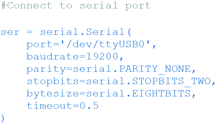
The next part defines the variable of our script which will allow the use of the serial port. Within the serial definition, six variables are set. The first, port, is the address to which commands should be sent and was found using the steps described above. The baudrate, parity, stopbits and bytesize are properties that are set by the equipment you are connecting to (those listed below correspond to the Vapourtec R2R4 system). Finally timeout defines how long your script should wait for a response from the equipment before closing the connection (we have found that half a second should be more than ample).
The third part comprises the class which powers the core of our web server. There are three function definitions within it, which correspond to the exposed ‘pages’ of the server. Any parameters which should be passed to each function are defined in the brackets alongside the function name.
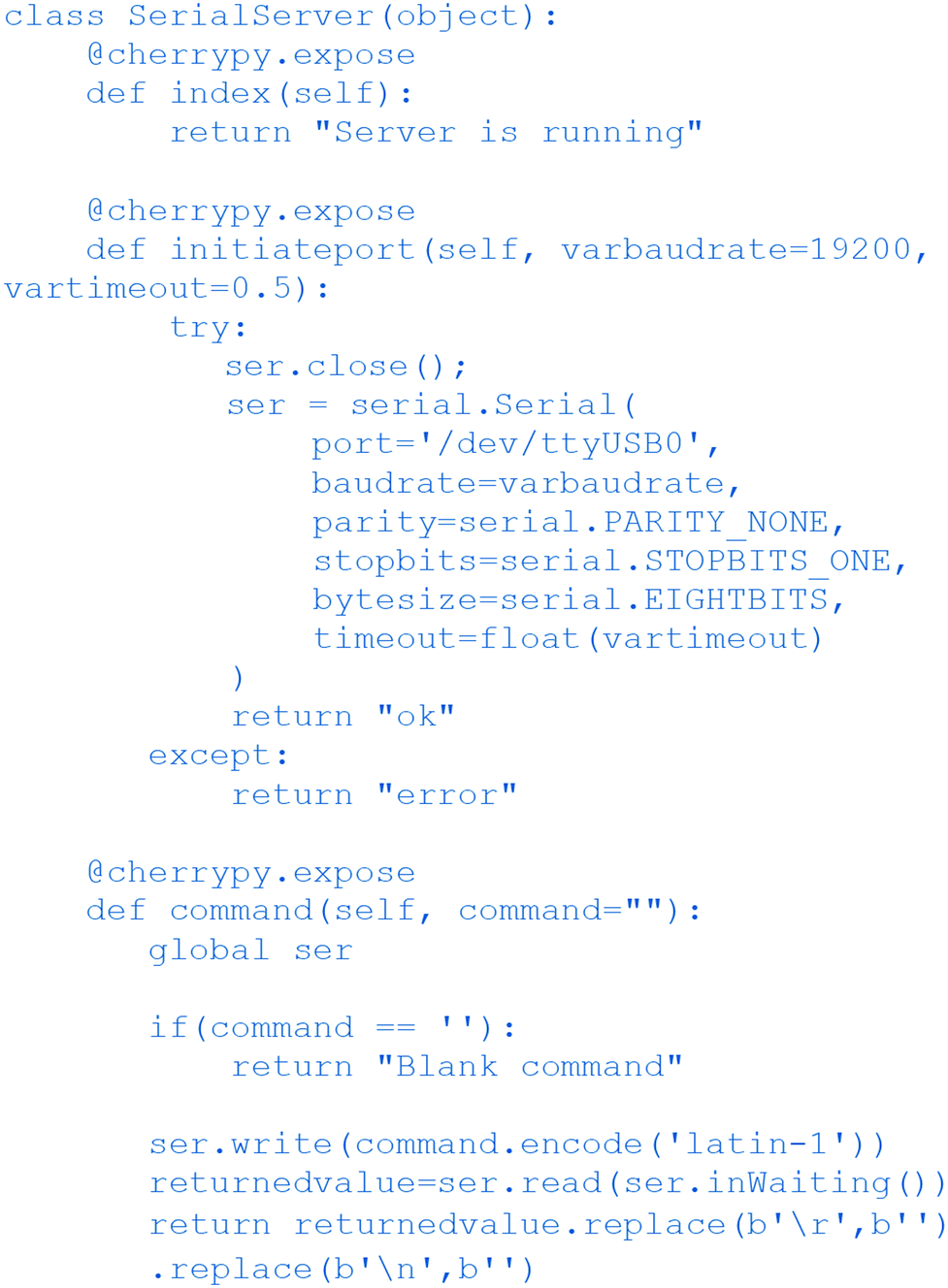
For example, if a request were sent to http://[Pi_IP_address]/initiateport?varbaudrate=9600&vartimeout=0.25 (e.g. by opening this in an internet browser on your phone) then our serial port definition would change to a baudrate of 9600 and a timeout of a quarter second. The server would then return ok if the settings were adjusted correctly, or error if something went wrong.
The first function, index, simply returns a message that the server is active to any requests that are sent to http://[Pi_IP_address]/.
The third function, command, is the most important for our script's functionality. It handles sending commands to the serial port and returning the response received from the equipment back to the request originator. The if statement has been included to prevent blank commands being sent accidentally to equipment. Within the ser.write line, any commands supplied through the applicable URL parameter are encoded using the latin-1 character set (from experience, our group has found that this avoids issues in some situations and so we recommend you include it too). Finally, the last line removes any new line and carriage return characters from the response collected from the equipment before returning the result to the requestor.
The fourth part of the script starts the server and starts listening for requests on port 80. If you wish to listen on a port different to the default HTTP, the first line can be adjusted to whichever number you wish (as long as it does not clash with a port already in use).
In order to test the script, put each of the code blocks above together into a.py script file on your Raspberry Pi and execute it. After a few seconds, you will be able to communication with your Pi using any device connected to the same local network. For example, having connected an R2R4 unit to the Pi you can turn it on remotely by opening http://[Pi_IP_address]/command?command=PN%0D%0A in an internet browser (the letters following the two percent symbols correspond to the URL encoded forms of the carriage return and new line characters respectively).
Section 5. Self-optimisation
Introduction to self-optimisation
A variety of different methods and algorithms exist for self-optimisation,30,31 usually originating from the disciplines of mathematics and computer science. The basic procedures followed by these algorithms are broadly similar: a series of conditions are trialled systematically, and the response of the system after each trial is used to select new trial conditions. The purpose of such a process is to maximise or minimise an output variable by changing input conditions without requiring intervention from operators during the optimisation process. In a synthesis context such a process might be targeted towards maximising yield, although multi-variable optimisations have been reported by our own group15,17 and others.32Commonly reported self-optimisation algorithms in the chemistry area include the simplex method and its derivatives,33 the SNOBFIT algorithm,32 Gaussian processes,34,35 and evolutionary methods.36 In this section we will describe in detail a simplex-derived method, known as the complex method.
While design of experiments (DoE) is not traditionally considered self-optimisation, as all experiment set points are defined at the beginning of the reaction process, it can be useful when exploring new chemical space. DoE procedures produce a mathematical model of a process output, for example reaction yield, as affected by various inputs, such as reaction temperature, across the defined chemical space. Accordingly DoE does not suffer from some of the more common setbacks associated with other self-optimisation techniques, such as identifying only a local maximum or minimum (which affects simplex-derived methods). Although further detail about DoE has not been included here, it is worth noting that a system could be constructed to automate DoE procedures using material covered in the earlier sections of this article.
Complex method
The complex method can be used to optimise a multicomponent, non-linear response within a constrained space.37 This algorithm changes the standard response of the system when determining new conditions to try, by extending or contracting reflected conditions depending on the relative performance of the most recent experiment. This contrasts with the original simplex method which follows only a repetitive reflection process to find an optimum.As an n-dimensional optimisation technique, the complex method is ideally suited to flow chemistry applications where it is possible to adjust any number of continuous variables within allowable limits to optimise a process outcome. From a discovery-level perspective, it provides a rapid and efficient means by which to find optimal experimental conditions and usually requires significantly fewer experiments to complete when compared with DoE-based approaches. However, it is worth noting that it suffers from the same limitations as the standard simplex method such as lack of exploration of the full chemical optimisation space and increased risk of identifying only a local maximum or minimum.
The evaluation function
Before the system can optimise a chemical reaction, it first needs something quantifiable that it can use to calculate the relative performance of a set of reaction conditions. In chemistry applications, usually this takes the form of a mathematical equation that gives an indication of yield using numerical detector feedback, such as that from a spectrometer. This equation is referred to by a variety of terms in literature, including objective function and optimisation function. Here we refer to it as the evaluation function.The algorithm itself
Before beginning a self-optimisation process, experimental parameters to be optimised must first be identified. Typically these include reaction temperature, residence time, overall concentration and stoichiometry. At the same time, the upper and lower allowable limits of each parameter must be chosen. This defines the chemical space within which the optimisation occurs. For example, you may like to optimise a reaction between the temperatures of 50 °C and 150 °C.While some literature reports select initial conditions on a random basis, this can lead to issues should points be clustered close together or lie close to boundary conditions.37 We recommend following a more defined selection process which selects points spread throughout the defined chemical space, as described below. No matter the method chosen to select conditions for initial iterations, a total of n + 1 iterations must be selected (where n is the number of parameters being optimised). For example, if you were conducting a 3-dimensional optimisation, where three experimental parameters were being optimised, then a total of four initial iterations must be selected.
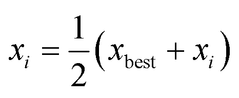
Conditions for the first iteration should lie at the centre of the chemical space, as found using:
 | (1) |
The coordinates of the remaining n iterations are found by first calculating the upper and lower quartiles of each parameter, before distributing experimental points throughout space while ensuring that the iterations do not all fall on a straight line or plane. This process can best be represented visually, as shown in Fig. 10, where the first iteration is positioned in the centre of available space and the remaining points are placed using quartile limits.
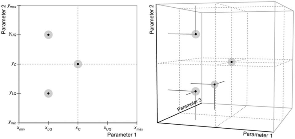 | ||
| Fig. 10 Plots of example two- and three-parameter optimisation experiments. Subscripts LQ, C and UQ refer to the lower quartile, centre and upper quartile values, respectively, across the axis range. The grey/black dots shown correspond to the initial n + 1 set points needed for optimisation. | ||
After a set of initial iterations has been defined, experiments are conducted using the set points for each. The performances of the reactions are calculated using the evaluation function, and each iteration is ranked from best to worst with the worst performing iteration, xw, being reflected through the centroid of an n-dimensional plane connecting the remaining n iterations (Fig. 11) to find the next set of conditions, xnext.
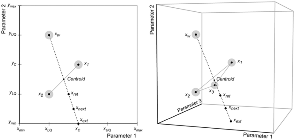 | ||
| Fig. 11 Example reflection process followed to select conditions for new iterations. These iterations fall on paths intersecting a plane within the n-dimensional space. | ||
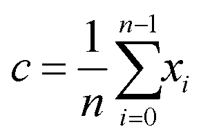
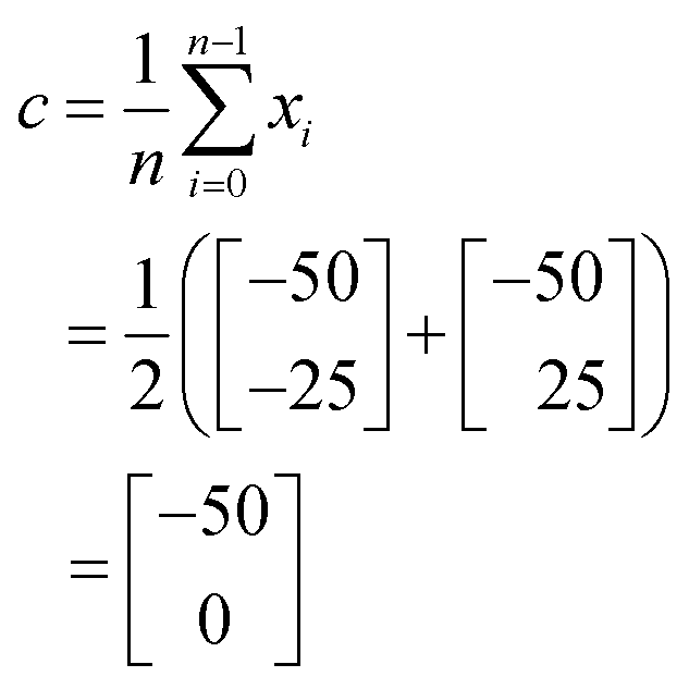
The position of the centroid, c, of the remaining iterations can be calculated using the equation:
 | (2) |
| xnext = (1 + α)c − αxw | (3) |
Having evaluated the performance of xnext, you can take one of three actions:
1. If this iteration is better than the second worst but worse than the best, remove the worst performing iteration from the current experiment set and perform a reflection using the second worst performing iteration. The reflection plane used to find the centroid includes the iteration just evaluated.
2. If this iteration was the best or equal to the best, then you are likely to be moving in the correct direction for optimisation and will thus you should perform an extension where the original reflection path is followed for an additional distance to find a new set of conditions xext. This new iteration is calculated using the equation:
| xext = γxnext + (1 − γ)c | (4) |
3. If this iteration was the worst or equal to the second worst, then you should perform a retraction where a new iteration is generated by moving back along the original path of reflection towards the centroid. The conditions for this retracted point xret are calculated using:
| xret = βxnext + (1 − β)c | (5) |
After most iterations, the above process is followed to determine new experimental conditions. There are only two scenarios that present exceptions to this procedure:
1. If the most recent iteration was determined through an extension process, and this iteration is the best performing, then the previous iteration (i.e. the iteration that led to the extension) is removed from the current experimental set and a reflection is performed.
2. If the most recent iteration was a retraction, and is the worst or equal to the second worst iteration, then a shrinking is performed where all but the best iterations in the current experimental set are moved towards the best performing by a factor of 0.5 to generate a new set of iterations:
 | (6) |
In the event that a calculated set point for an experiment parameter falls outside the allowed chemical space, replace this set point with the relevant parameter limit.
The above steps are repeated until an optimum is found.
We recommend that a modified form of the convergence checking procedure first proposed by Nelder and Mead when describing the original simplex algorithm.38 Before checking for convergence, we recommend that a sufficiently large number of iterations are carried out (usually n + 4), after which time the mean and variance of the evaluated responses in the current experimental set are calculated. You should then compare the ratio of the variance to the mean against a predefined convergence criterion (ξ):
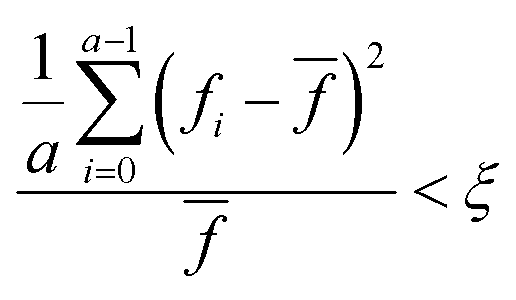 | (7) |
![[f with combining macron]](https://www.rsc.org/images/entities/i_char_0066_0304.gif) is the mean evaluated response in the current experimental set. We recommend that ξ is set to around 0.05 (or 5%).
is the mean evaluated response in the current experimental set. We recommend that ξ is set to around 0.05 (or 5%).
When this convergence criterion is met, it indicates that the differences in evaluated response between each iteration is sufficiently small that no further improvements can be obtained by continuing the optimisation process.
Worked example
For this worked example, we will manually optimise eqn (8) within the limits of a and b as shown underneath. You may like to create a Python or C script to speed this process along, but performing calculations by hand will give a good feel for how the optimisation process works.| z = (4a + b)2 | (8) |
Find the optimal (highest z) for:
| a: −75 to 25 |
| b: −50 to 50 |
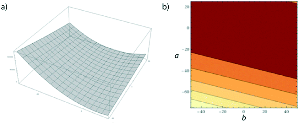 | ||
| Fig. 12 a) Surface plot given by eqn (8); b) contour plot showing a top-down view of (a). | ||
The general steps for approaching this problem are as follows:
1. Find the conditions for the initial n + 1 iterations.
2. Carry out experiments at each point, evaluating performance using the evaluation function.
3. Rank from best to worst.
4. Follow the process described above to determine the conditions for the next iteration (e.g. reflection).
5. Repeat the process above until iterations converge.
In this case, as a 2-dimensional optimisation, a total of three initial conditions need to be chosen. The first is placed at the centre of the optimisation space, as found using eqn (1):
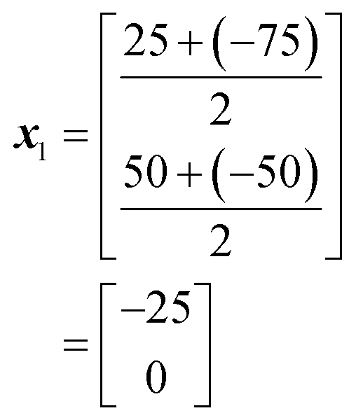
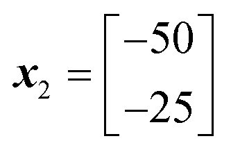
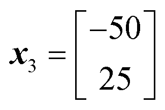
The positions of the n + 1 initial conditions are shown in Fig. 13a. To evaluate the performance of each iteration we can simply insert the values of a and b for each iteration into eqn (8), to give the values below. In a synthesis context, some form of detector feedback would need to be incorporated having conducted actual experiments using each iteration, contrasting with the purely mathematical nature of this example.
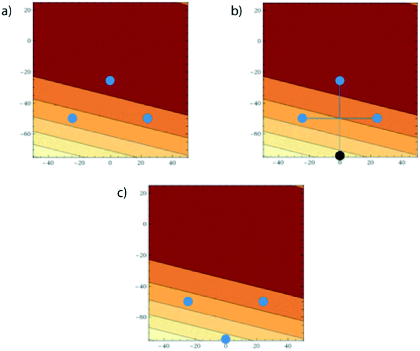 | ||
| Fig. 13 a) The initial n + 1 conditions (corresponding to x1, x2 and x3); b) the worst performing iteration is reflected through a line connecting the remaining two to give x4 (shown in black); c) the current experimental set following the evaluation of x4 and subsequent removal of x1. | ||
x
1 evaluated performance: 10![[thin space (1/6-em)]](https://www.rsc.org/images/entities/char_2009.gif) 000 000 |
|
x
2 evaluated performance: 50625 |
|
x
3 evaluated performance: 30625 |
Evaluating the performance of x4 gives a result of 90
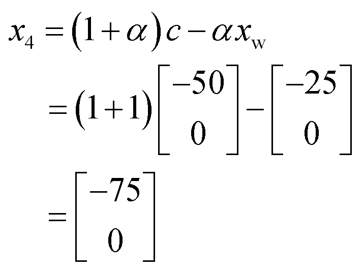 000. As this is better performing than x1, we can remove x1 from the current experimental set leaving the new current experimental set as shown in Fig. 13c. As it turns out x4 is the best performing of all iterations thus far, and so the complex method calls for an extension to be conducted where a new iteration is found further along the line connecting x1 and x4. However, in this case x4 is placed at the edge of the allowable optimisation space and so there is no point to calculate x5 using an extension as it would be returned to the exact position as x4.
Accordingly the position of x5 can be calculated by taking a reflection of x3 (the worst performing of the current experimental set) through the centroid of the line connected x2 and x4, giving the coordinates (Fig. 14):
 | ||
| Fig. 14 Reflection process to find position of x5. | ||
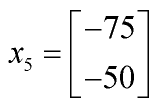 500.
500.
This lies directly in the corner of our allowable optimisation space and so cannot be optimised further, given the shape of the response curve in Fig. 12. However, in a live experiment we would not know the response curve and thus would not know that it would not be possible to optimise beyond this point. The next steps therefore are to perform a shrinking (as before an extension at this time can be avoided, as x5 lies at the extremes of both parameters).
This would give the positions of two new iterations as below:
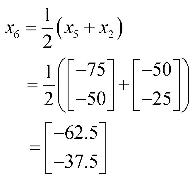
Which evaluate to 82
 656.25 and 105625, respectively. As x5 is still the best performing, another shrinking is performed to give the conditions for more iterations. This process is repeated until your convergence criterion is met, with x5 giving the best results in this example no matter how stringent a value ξ is assigned.
Applying to a synthetic environment
While the worked example above is purely mathematical, it is relatively straightforward to transfer the process into a chemical environment. Such a well-defined governing equation that was optimised (eqn (8)) of course does not exist in a reaction context; however, we do not need it to. It's possible to treat the reaction itself as a ‘black box’ function where inputs (reaction parameters such as temperature) give a defined output (e.g. yield or conversion) which can be measured using in-line or on-line detectors such as the Mettler-Toledo FlowIR39 or an LCMS stack.By following the complex method process, new input conditions will be generated after which detector feedback can be fed into the evaluation function to determine how well a certain iteration has performed (e.g. by calculating a ratio between products and starting materials), driving the systematic generation of new iterations to try.
Material covered in the first sections of this paper can be used to connect to reaction equipment such as pumps, reactor systems and detectors to control parameters and gather information necessary for optimisation. Indeed, for all cases of our own reported self-optimisation work this process was followed.15,17
Conclusions
To derive most benefit from the above Tutored Discourse, we would now encourage transfer of this knowledge to real-time experimentation to build confidence and trust in the systems. Only through this increased exposure and practice can the capabilities and opportunities be fully recognised to lead to future innovations in autonomous reaction control and discovery. Eventually all these systems should be available through open-source40 repositories, such as GitHub, and managed through normal electronic laboratory notebook (ELN) methods.Conflicts of interest
There are no conflicts to declare.Acknowledgements
The authors gratefully acknowledge financial support from the H2020-FETOPEN-2016-2017 programme of European commission (grant agreement number: 737266-ONE FLOW).Notes and references
- S. V. Ley, D. E. Fitzpatrick, R. J. Ingham and R. M. Myers, Angew. Chem., Int. Ed., 2015, 54, 3449–3464 CrossRef CAS PubMed.
- S. V. Ley, D. E. Fitzpatrick, R. M. Myers, C. Battilocchio and R. J. Ingham, Angew. Chem., Int. Ed., 2015, 54, 10122–10136 CrossRef CAS PubMed.
- C. W. Coley, D. A. Thomas, J. A. M. Lummiss, J. N. Jaworski, C. P. Breen, V. Schultz, T. Hart, J. S. Fishman, L. Rogers, H. Gao, R. W. Hicklin, P. P. Plehiers, J. Byington, J. S. Piotti, W. H. Green, A. J. Hart, T. F. Jamison and K. F. Jensen, Science, 2019, 365, eaax1566 CrossRef CAS PubMed.
- M. Yan, Y. Kawamata and P. S. Baran, Angew. Chem., Int. Ed., 2018, 57, 4149–4155 CrossRef CAS PubMed.
- P. Koos, D. L. Browne and S. V. Ley, Green Process. Synth., 2012, 1, 11–18 CAS.
- M. O'Brien, P. Koos, D. L. Browne and S. V. Ley, Org. Biomol. Chem., 2012, 10, 7031–7036 RSC.
- D. X. Hu, M. O'Brien and S. V. Ley, Org. Lett., 2012, 14, 4246–4249 CrossRef CAS PubMed.
- S. V. Ley, R. J. Ingham, M. O'Brien and D. L. Browne, Beilstein J. Org. Chem., 2013, 9, 1051–1072 CrossRef CAS PubMed.
- R. J. Ingham, C. Battilocchio, J. M. Hawkins and S. V. Ley, Beilstein J. Org. Chem., 2014, 10, 641–652 CrossRef PubMed.
- S. Glöckner, D. N. Tran, R. J. Ingham, S. Fenner, Z. E. Wilson, C. Battilocchio and S. V. Ley, Org. Biomol. Chem., 2015, 13, 207–214 RSC.
- R. J. Ingham, C. Battilocchio, D. E. Fitzpatrick, E. Sliwinski, J. M. Hawkins and S. V. Ley, Angew. Chem., Int. Ed., 2015, 54, 144–148 CrossRef CAS PubMed.
- K. Molga, E. P. Gajewska, S. Szymkuć and B. A. Grzybowski, React. Chem. Eng., 2019, 4, 1506–1521 RSC.
- S. V. Ley, D. E. Fitzpatrick, R. J. Ingham and N. Nikbin, Beilstein Mag., 2015, vol. 1, DOI:10.3762/bmag.2.
- D. E. Fitzpatrick, C. Battilocchio and S. V. Ley, ACS Cent. Sci., 2016, 2, 131–138 CrossRef CAS PubMed.
- D. E. Fitzpatrick, C. Battilocchio and S. V. Ley, Org. Process Res. Dev., 2016, 20, 386–394 CrossRef CAS.
- D. E. Fitzpatrick and S. V. Ley, React. Chem. Eng., 2016, 1, 629–635 RSC.
- D. E. Fitzpatrick, T. Maujean, A. C. Evans and S. V. Ley, Angew. Chem., Int. Ed., 2018, 57, 15128–15132 CrossRef CAS PubMed.
- P. L. Urban, Angew. Chem., Int. Ed., 2018, 57, 11074–11077 CrossRef CAS PubMed.
- C.-L. Chen, T.-R. Chen, S.-H. Chiu and P. L. Urban, Sens. Actuators, B, 2017, 239, 608–616 CrossRef CAS.
- For more information about the One-Flow research programme, refer to https://one-flow.org/ [Date Accessed: 27/08/19].
- A brief introduction to the Linux command line can be found online at https://maker.pro/linux/tutorial/basic-linux-commands-for-beginners [Date Accessed: 27/08/19].
- Full listings of available Arduino libraries are shown at https://www.arduino.cc/en/reference/libraries [Date Accessed: 27/08/19].
- D. E. Fitzpatrick and S. V. Ley, Tetrahedron, 2018, 74, 3087–3100 CrossRef CAS.
- K.-T. Hsieh and P. L. Urban, RSC Adv., 2014, 4, 31094–31100 RSC.
- M. O'Brien, I. R. Baxendale and S. V. Ley, Org. Lett., 2010, 12, 1596–1598 CrossRef PubMed.
- OpenCV, [Date Accessed: 27/08/19] https://opencv.org/.
- SimpleCV, [Date Accessed: 27/08/19] http://simplecv.org/download/.
- D. E. Fitzpatrick, R. J. Mutton and S. V. Ley, React. Chem. Eng., 2018, 3, 799–806 RSC.
- CherryPy, [Date Accessed: 27/08/19] https://cherrypy.org/.
- A. D. Clayton, J. A. Manson, C. J. Taylor, T. W. Chamberlain, B. A. Taylor, G. Clemens and R. A. Bourne, React. Chem. Eng., 2019, 4, 1545–1554 RSC.
- D. C. Fabry, E. Sugiono and M. Rueping, Isr. J. Chem., 2014, 54, 341–350 CrossRef CAS.
- A. M. Schweidtmann, A. D. Clayton, N. Holmes, E. Bradford, R. A. Bourne and A. A. Lapkin, Chem. Eng. J., 2018, 352, 277–282 CrossRef CAS.
- S. N. Deming, L. R. Parker and M. B. Denton, Crit. Rev. Anal. Chem., 1978, 7, 187–202 CAS.
- N. Peremezhney, E. Hines, A. Lapkin and C. Connaughton, Eng. Optim., 2014, 46, 1593–1607 CrossRef.
- C. Houben and A. A. Lapkin, Curr. Opin. Chem. Eng., 2015, 9, 1–7 CrossRef.
- T. C. Le and D. A. Winkler, Chem. Rev., 2016, 116, 6107–6132 CrossRef CAS PubMed.
- R. F. Kazmierczak Jr., SSRN Electron J., 1997, 21996, DOI:10.2139/ssrn.15071.
- J. A. Nelder and R. Mead, Comput. J., 1965, 7, 308–313 CrossRef.
- C. F. Carter, H. Lange, S. V. Ley, I. R. Baxendale, B. Wittkamp, J. G. Goode and N. L. Gaunt, Org. Process Res. Dev., 2010, 14, 393–404 CrossRef CAS.
- M. O'Brien, L. Konings, M. Martin and J. Heap, Tetrahedron Lett., 2017, 58, 2409–2413 CrossRef.
Footnote |
| † Electronic supplementary information (ESI) available: Appendices and additional Python script examples. See DOI: 10.1039/c9re00407f |
| This journal is © The Royal Society of Chemistry 2020 |