
 Open Access Article
 This Open Access Article is licensed under a Creative Commons Attribution-Non Commercial 3.0 Unported Licence
Data-driven prediction and control of wastewater treatment process through the combination of convolutional neural network and recurrent neural network
Zhiwei Guo a,
Boxin Dub,
Jianhui Wanga,
Yu Shenae,
Qiao Lib,
Dong Fengc,
Xu Gaoac and
Heng Wang*d
a,
Boxin Dub,
Jianhui Wanga,
Yu Shenae,
Qiao Lib,
Dong Fengc,
Xu Gaoac and
Heng Wang*d
aNational Research Base of Intelligent Manufacturing Service, Chongqing Technology and Business University, Chongqing 400067, P. R. China
bSchool of Economics, Chongqing Technology and Business University, Chongqing 400067, P. R. China
cChongqing Sino French Environmental Excellence Research & Development Center Co., Ltd, Chongqing 400042, P. R. China
dCollege of Mechanical and Electrical Engineering, Henan Agricultural University, Zhengzhou 450002, P. R. China. E-mail: dawn_wangh@163.com
eChongqing South-to-Thais Environmental Protection Technology Research Institute Co., Ltd., Chongqing 400069, China
First published on 1st April 2020
Abstract
It is widely believed that effective prediction of wastewater treatment results (WTR) is conducive to precise control of aeration amount in the wastewater treatment process (WTP). Conventional biochemical mechanism-driven approaches are highly dependent on complicated and redundant model parameters, resulting in low efficiency. Besides, sharp increase in business volume of wastewater treatment requires automatic operation technologies for this purpose. Under this background, researchers started to introduce the idea of data mining to model the WTP, in order to automatically predict WTR given inlet conditions and aeration amount. However, existing data-driven approaches for this purpose focus on modelling of the WTP at independent timestamps, neglecting sequential characteristics of timestamps during the long-term treatment process. To tackle the challenge, in this paper, a novel prediction and control framework through combination of convolutional neural network (CNN) and recurrent neural network (RNN) is proposed for prediction of the WTR. Firstly, the CNN model is utilized to automatically extract the local features of each independent timestamp in the WTP and make them encoded. Next, the RNN model is employed to represent global sequential features of the WTP on the basis of local feature encoding. Finally, we conduct a large number of experiments to verify efficiency and stability of the proposed prediction framework.
1. Introduction
The past decade has witnessed great progress in various fields of contemporary society, also arousing public attention to the topic of environmental protection in which wastewater treatment acts as the most important one.1,2 The most universal solution for the wastewater treatment process (WTP) is the utilization of biochemical methods, almost all of whom take the amount of dissolved oxygen as a key parameter.3–5 Specifically, pollutants can be treated by adding a certain amount of dissolved oxygen derived from industrial aeration.6,7 The precise control of aeration amount has been a main concern in the field of chemistry for a long period, because it will exert influence on effects and results of the treatment process.8,9 Thus, there is no doubt that effective prediction of wastewater treatment results (WTR) will conversely contribute a lot to precise control of aeration amount in the WTP.10,11However, making precise predictions on WTR remains a challenging task.12,13 As is known, WTP is essentially a complex system process accompanied with internal particle movement as well as invisible uncertainty, because of the occurrence of various imperceptible biochemical reaction among different chemical substances.14–16 Conventional biochemical mechanism-driven approaches for this purpose are highly dependent on complicated and redundant model parameters, which usually results in inefficient operations due to the limitation of manual computation capability.17–19 Besides, the rapid growth of economy also brings about a sharp increase in volume of wastewater production, further requiring innovative schemes to generate precise control strategy for WTP through technical means of high performance computation.20–22
Fortunately, longing and yearning of people to intelligence breeds some newly emerging technologies such as artificial intelligence, which profoundly facilitates the solution of cross-domain issues.23,24 As a primary branch of artificial intelligence, data mining technology manages to discover hidden information and predict future tendencies from a large amount of historical data by means of statistical learning methods, and has been applied to many industrial scenarios to solve various engineering problems.25,26 From the perspective of mathematical modelling, WTP can be abstracted as a grey box model with observed results and unobserved intermediate rules. Data-driven models, characterized by excellent capability of feature extraction and cognitive computation, are well suitable for representation of the WTP.27,28
In fact, data-driven modelling for WTP has attracted more and more research attention, and a number of representative solutions have been put forward during past few years. The earliest of them are built upon the basis of numerical methods and have not yet introduced idea of AI. For example, Krueger et al.29 adopted key performance indicator30 to come up with a data-driven method for this purpose, and Shao et al.31 proposed a variant of least squares model to predict outlet quality in advance. Due to the superficial expression of complex biochemical process provided by conventional mathematical methods, researchers gradually explore new solutions. Neural network, a kind of data mining algorithms for distributed parallel information processing, imitates the behaviour characteristics of brain neurons of animals to realize high-performance computation. Owing to its ultra-high sensitivity easily adaptive to potentially complex processes, neural network model has been extended for a variety of industrial scenarios containing the WTP in recent years.32–34 Sridevi et al.32 proposed a modified backpropagation neural network model that is able to adaptively set up learning rate for estimation of outlet status. Hassen et al.33 took artificial neural network into account, and employed a feed-forward, back propagation learning method to predict results of the WTP. Sadeghassadi et al.34 managed to present an optimal variable setpoint and a setpoint-tracking control loop, so as to well control the WTP. In order to enforce ability of inference, some researchers also investigated coupling of neural network and fuzzy logic which is an effective mathematical reasoning tool.35–39 For instance, Yang et al.35 proposed a fuzzy neural network-based predictive control mechanism for WTP and proved its superiority through simulation experiments. Ruan et al.36 introduced fuzzy neural network model into an anaerobic digestion system, and evaluated the performance of such model in predicting WTR. Qiao et al.37 presented an adaptive fuzzy neural network-based control system framework for multi-objective WTP. The proposed control system contains two parts: an optimization module and an adaptive fuzzy neural network. Zhou et al.38 proposed a self-organizing fuzzy neural network method and utilized it to design a control system for dissolved oxygen in WTP. Besides, Han et al.39 also proposed an improved multi-objective optimal controller related to Qiao et al. And to pursue a faster convergence speed of models, wavelet transformation theory is also integrated into neural network model for prediction of WTR.40–42 Loussifi et al.40 proposed a hybrid computational strategy that combines kernel methods with fuzzy wavelet network to realize prediction of WTR. Huang et al.41 presented a fuzzy wavelet neural network model for WTP and really accelerates processing speed. Cong et al.42 exploited adaptive weighted fusion and wavelet neural network model to construct an estimation method for WTR.
But almost all of the existing approaches were established upon the assumption that treatment processes at different timestamps are mutually independent, mainly focusing on modelling of WTP at different timestamps. Nevertheless, treatment processes at different timestamps are actually an evolving sequence, and there exists sequential correlations among them. In particular, biochemical reaction at one timestamp is accompanied with change of materials and energy, which will certainly influence the treatment process at next timestamp. Therefore, data-driven modelling for WTP is required to be extended by taking global sequential dependency characteristics into consideration.
To overcome this challenge, this research explores to realize prediction of WTR with integration of both local process factors and global sequential factors. In this paper, a novel Prediction and Control framework with the mixture of Convolutional neural network and Recurrent neural network (PC-CR) is proposed for this purpose. Firstly, convolutional neural network (CNN) model is designed to automatically extract local features of each independent timestamp in the WTP and make them encoded. The CNN consists of three layers: convolutional layer, pooling layer and full connection layer, responsible for encoding initial features. Next, recurrent neural network (RNN) model is employed to deeply represent global sequential features of the WTP on the basis of local feature encoding. Prediction results can be generated accordingly as outputs of the RNN. Finally, we conduct a large amount of computational experiments on real-world dataset to evaluate both efficiency and stability of the proposed PC-CR framework. To the best of our knowledge, we are the first to realize data-driven prediction of WTR considering effect of global sequential features. Main contributions of this paper are summarized as follows:
(1) We illustrate the existence of time-series characteristics in WTP and recognize the limitation of existing data-driven methods.
(2) We propose a novel mechanism PC-CR for WTP to automatically predict treatment results given inlet conditions and aeration amount.
(3) We empirically evaluate efficiency and stability of the proposed PC-CR on a real-world dataset acquired from a sewage treatment plant.
The remainder of this paper is organized as follows. Section 2 gives overview of the research problem and framework. Detailed mathematical process of methodology is described in Section 3. In Section 4, a large amount of experiments are conducted to evaluate efficiency and stability of the proposed PC-CR. And we conclude this paper in Section 5.
2. Overview
2.1 Problem statement
The experimental dataset utilized in this research was collected from an A2/O process-based sewage treatment plant located in Nan'an District, Chongqing, China. Among, A2/O process refers to anaerobic-anoxic-oxic process, and is a common secondary sewage treatment process that makes wastewater flow through anaerobic process, anoxic process and oxic process in sequence. Fig. 1 illustrates process structure of this sewage treatment plant, and we propose to define core terms of it as follows: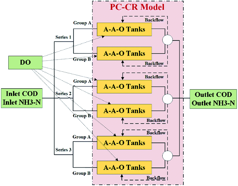 | ||
| Fig. 1 Process structure of the sewage treatment plant. | ||
Definition 1 (inlet COD): initial index of the chemical oxygen demand (COD) before entering into treatment tanks.
Definition 2 (inlet NH3–N): initial index of the ammonia nitrogen (NH3–N) before entering into treatment tanks.
Definition 3 (DO): the dissolved oxygen (DO) added into A2/O treatment tanks.
Definition 4 (outlet COD): final index of the chemical oxygen demand (COD) after treatment tanks.
Definition 5 (outlet NH3–N): final index of the ammonia nitrogen (NH3–N) after treatment tanks.
It can be intuitively observed from Fig. 1 that COD and NH3–N are viewed as two major pollutant indexes to be treated, and that treatment process is implemented through adjusting amount of DO added into A2/O treatment tanks in immediate process. There are totally eighteen treatment tanks in the sewage treatment plant, and all of whom are divided into three series in which each series contains two groups of A-A-O treatment tanks. Collection of the dataset is implemented through deploying sensors in all the key infrastructures to monitor amount values of above five indexes, and time span of the dataset is from July 2018 to June 2019. At the end of each series, sludge is launched a backflow according to a certain proportion. Given inlet pollutant indexes, the goal of this research is to formulate a PC-CR mechanism that mathematically express the immediate A-A-O treatment processes and predict outlet pollutant indexes according to inlet conditions and configuration amount of DO in each tank. Also, it is supposed to note that PC-CR mechanism is established on the basis of following three assumptions:
Assumption 1: treatment tanks in different groups are mathematically independent and hardly have internal connections during treatment processes.
Assumption 2: as backflow ratio is constantly set to 300% and never changes, the impact of it can be ignored.
Assumption 3: as measurement units of outlet COD and outlet NH3–N are mg L−1, inlet flowrate of the sewage treatment plant is viewed nearly constant.
2.2 Framework
Fig. 2 demonstrates framework of the proposed PC-CR mechanism. The amount of DO added in eighteen tanks at the t-th timestamp are denoted as xij(t) (i = 1,2,…,6; j = 1,2,3), where i denotes the six groups and j denotes the three tanks of each group. The total xij(t) can be finally aggregated into a feature matrix X(t) who will be input into CNN model to be encoded into a feature vector O(t) (t = 1,2,…,T). Then, the O(t) is regarded as input of each timestamp in RNN model and further encoded into a hidden layer vector ht. Finally, the real-world dataset is input to train the PC-CR mechanism to make it have the ability of prediction. Thus, given inlet pollutant indexes at the n + 1-th timestamp, once configuration amount of DO at the timestamp is determined, outlet pollutant indexes will be correspondingly predicted by the PC-CR.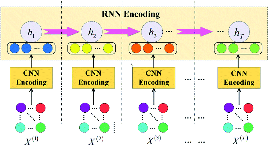 | ||
| Fig. 2 Framework of the PC-CR mechanism. | ||
3. Methodology
3.1 CNN encoding
In recent years, CNN method has shown an excellent performance in terms of automatic feature extraction and deep feature representation. Therefore, we develop a CNN model to represent features of initial data, and flowchart of the CNN model is shown as Fig. 3. | ||
| Fig. 3 Flowchart of the developed CNN model. | ||
The feature matrix at the t-th timestamp X(t) is a 6 × 3-dimensional matrix, and is concatenated with feature matrix at the t − 1-th timestamp X(t−1) to construct a new 6 × 6-dimensional feature matrix, which is represented as:
| Xnew(t) = X(t) ⊕ X(t−1) | (1) |
The new feature matrix Xnew(t) is then input into convolutional layer for convolutional computation which is an inner product operation between matrix Xnew(t) and a series of M-core 3 × 3-dimensional filtering matrices Fm(t) (m = 1,2,…,M). Note that Fm(t) is a group of matrices with size number of M. Output of convolutional computation is a new feature expression E(t) who is a series of M-core 4 × 4-dimensional matrices calculated as:
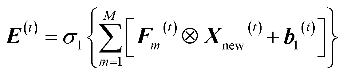 | (2) |
| σ1(x) = max(0,x) | (3) |
Similarly, E(t) is a group of matrices with size number of M.
The role of pooling layer is to lower down dimensions of matrices in E(t) and generate a more compact representation of them. Here, the most common max pooling method is utilized in this research, meaning that maximum values in each separated pooling block are selected as local feature values to form anther series of M-core 2 × 2-dimensional matrices Epool(t). The illustration of pooling process is shown in Fig. 3.
The last layer is full connection layer, where a linear mapping function is formulated to generate a more abstract vectorized expression as follows:
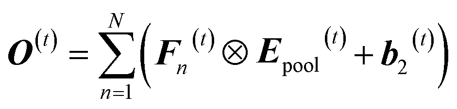 | (4) |
3.2 RNN encoding
In recent years, RNN has shown an outstanding performance in terms of sequential characteristics modelling. As a modified version of RNN, Long Short-Term Memory (LSTM) model is specially designed to solve the long-term dependence problem confronted by general RNN methods. LSTM is uniquely added a memory storage module that is protected by some gating neurons who are distinguished from ordinary neurons by setting two states: on and off. Therefore, LSTM is formulated in this research to model sequential characteristics of WTP. Detailed flowchart of the LSTM model is shown as Fig. 4.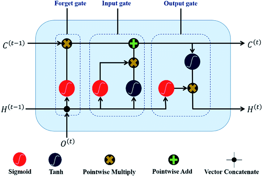 | ||
| Fig. 4 Flowchart of the LSTM model. | ||
It can be observed from the Fig. 4 that the LSTM comprises forget gate, input gate and output gate. The forget gate determines how much of the long-term unit state at the previous timestamp C(t−1) is retained to current moment C(t). The input gate determines how much of the input O(t) is saved to the unit state C(t) at the t-th timestamp. The output gate is used to control how much of the unit state C(t) is transferred to network output H(t).
As for the forget gate, its control factor at the t-th timestamp is calculated as:
| f(t) = σ2{Wf(t)[H(t−1),O(t)] + bf(t)} | (5) |
 | (6) |
The f(t) is a real number ranging from 0 and 1. f(t) = 0 denotes the status that historical information is completely forgotten, and f(t) = 1 denotes the status that historical information is completely remembered.
As for the input gate, its status vector is updated as follows:
| u(t) = σ2{Wu(t)[H(t−1),O(t)] + bu(t)} | (7) |
C(t) = f(t)C(t−1) + u(t)![[C with combining tilde]](https://www.rsc.org/images/entities/b_i_char_0043_0303.gif) (t) (t)
| (8) |
(t) is candidate value generated by tanh operator and is computed as:|
(t) = tanh{WC(t)[H(t−1),O(t)] + bC(t)}
| (9) |
As for the output gate, its control factor at the t-th timestamp is calculated as:
| v(t) = σ2{Wv(t)[H(t−1),O(t)] + bv(t)} | (10) |
H(t) = v(t)![[thin space (1/6-em)]](https://www.rsc.org/images/entities/char_2009.gif) tanh[C(t)] tanh[C(t)]
| (11) |
3.3 Decoding
As each group of operating results produce an output H(t), operating results of multiple groups are demonstrated as:| Hl(t) = {H1(t),H2(t),…,HL(t)} | (12) |
| ŷl(t) = σ2{θ[Hl(t)]} | (13) |
| al(t) = σ3{φ[Hl(t)]} | (14) |
| σ3(x) = max(0.01x,x) | (15) |
The two weight factors are conducted inner-product operations into a total weight vector as:
| yl(t) = al(t)ŷl(t) | (16) |
The overall prediction is a linear transformation of yl(t), which is represented as:
| ẑl(t) = σ2{Wyl(t)yl(t) + byl(t)} | (17) |
 | (18) |
 | (19) |
After that, a complete prediction mechanism is established for outlet indexes. Once values of inlet indexes at the t + 1-th timestamp are input, the predicted values of outlet indexes at this timestamp will be obtained accordingly.
4. Experiments and analysis
4.1 Data pre-processing
In order to evaluate performance of the proposed PC-CR mechanism, a series of experiments are conducted on the real-world dataset collected from a sewage treatment plant that has been mentioned in Section 2.1. Due to frequency inconsistency of daily monitoring, we uniformly select the first 200 pieces of data during each day. Referring to the structure in Fig. 1, symbolic notations and statistical characteristics of the dataset are respectively listed in Tables 1 and 2.| Variable | Definition |
|---|---|
| x1j, x2j | DO density values of three tanks in Group A and Group B of Series 1 |
| x3j, x4j | DO density values of three tanks in Group A and Group B of Series 2 |
| x5j, x6j | DO density values of three tanks in Group A and Group B of Series 3 |
| α1, α2 | Density values of inlet COD and inlet NH3–N |
| β1, β2 | Density values of outlet COD and outlet NH3–N |
| Variable | Min | Max | Mean | SD |
|---|---|---|---|---|
| x1j (mg L−1) | 1.002 | 9.562 | 2.810 | 1.519 |
| x2j (mg L−1) | 1.000 | 9.287 | 3.293 | 1.861 |
| x3j (mg L−1) | 1.001 | 9.413 | 2.607 | 1.117 |
| x4j (mg L−1) | 1.000 | 9.088 | 2.691 | 1.109 |
| x5j (mg L−1) | 1.003 | 9.956 | 5.571 | 2.604 |
| x6j (mg L−1) | 1.241 | 9.973 | 6.152 | 3.118 |
| α1 (mg L−1) | 9.339 | 1061.544 | 441.008 | 195.165 |
| α2 (mg L−1) | 0.156 | 110.467 | 27.283 | 9.889 |
| β1 (mg L−1) | 3.016 | 49.475 | 25.606 | 0.317 |
| β2 (mg L−1) | 0.156 | 28.607 | 2.215 | 0.703 |
Fig. 5 contains two subfigures, respectively visualizing more intuitive statistical characteristics and distribution characteristics of DO density values in immediate A-A-O process. Among, POOL1-A3, POOL1-B3, POOL2-A3, POOL2-B3, POOL3-A3, POOL3-B3 separately refers to variable x1j, x2j, …, x6j. We further compute Pearson correlation coefficients of these variable pairs and visualize them as Fig. 6, in which gradual change of colour from blue to red reflects the gradual change of correlation degree.
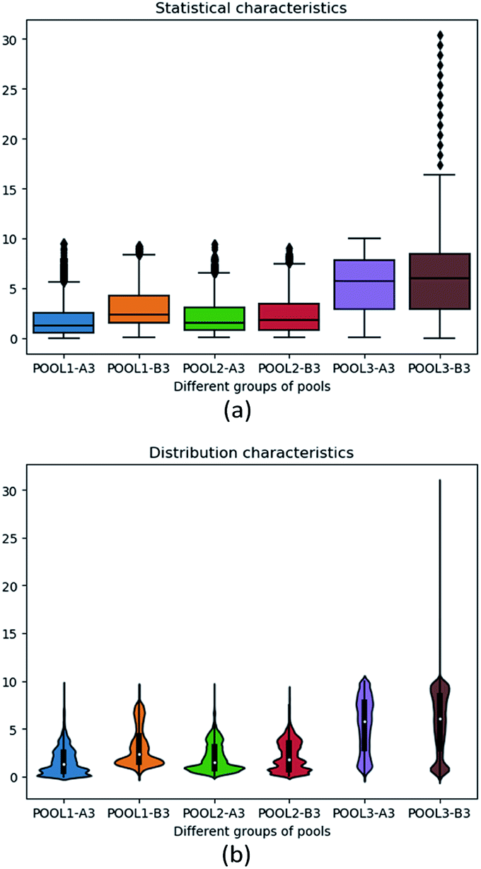 | ||
| Fig. 5 (a) Statistical and (b) distribution characteristics of six groups of DO density values. | ||
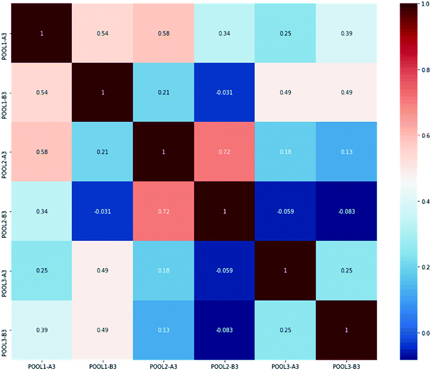 | ||
| Fig. 6 Correlation coefficients among six groups of DO density values. | ||
In all, two aspects of phenomenon can be observed from above figures and tables. For one thing, variables are evenly distributed in specific ranges, which is suitable for data-driven modelling. For another, correlation values of variable pairs are relatively small and almost lower than 0.1, which satisfies Assumption 2 in Section 2.1. Therefore, the pre-processed dataset is well suited for evaluation of the proposed PC-CR.
4.2 Experimental settings
In order to assess performance from the perspective of quantification, two widely used evaluation metrics are utilized in our experiments to measure prediction accuracy: mean absolute error (MAE),44 root mean square error (RMSE).45 Their expressions are given as:
 | (20) |
 | (21) |
![[small beta, Greek, circumflex]](https://www.rsc.org/images/entities/i_char_e114.gif) γ is predicted values, and
γ is predicted values, and  is the total size of testing values. Clearly, as for these two metrics, lower values denote better performance.
The proposed PC-CR needs to be compared with baseline methods concerning above three metrics. We select several existing data-driven prediction methods for WTR: CNN,46 LSTM,47 FNN,35 WFNN.41 CNN and LSTM respectively denotes standard CNN model and standard LSTM model. FNN and WFNN respectively refers to fuzzy neural network model and wavelet fuzzy neural network model that have been briefly introduced in Section 1. Main ideas and workflow of these baseline methods are described in corresponding literatures.
The PC-CR and baselines are implemented using the programming language Python on a GPU-equipped workstation. Parameters M and N in eqn (2) and (4), trade-off parameter λ in eqn (19), and the learning rate in RMSProp are set to multiple groups of values during the process of experiments. M and N are initially set to 40 and 96, λ is firstly set to 0.5, and learning rate are firstly set to 0.01. Besides, the experimental dataset is split into training set and testing set two parts. Training set plays the role of estimating model parameters and setting up prediction model, while testing set is adopted to test performance of prediction methods which can be assessed through aforementioned three evaluation metrics. Proportions of training set and testing set are set to 70% and 30% initially, and will also change multiple times.
4.3. Results and analysis
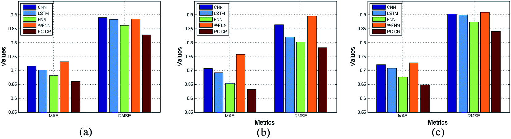
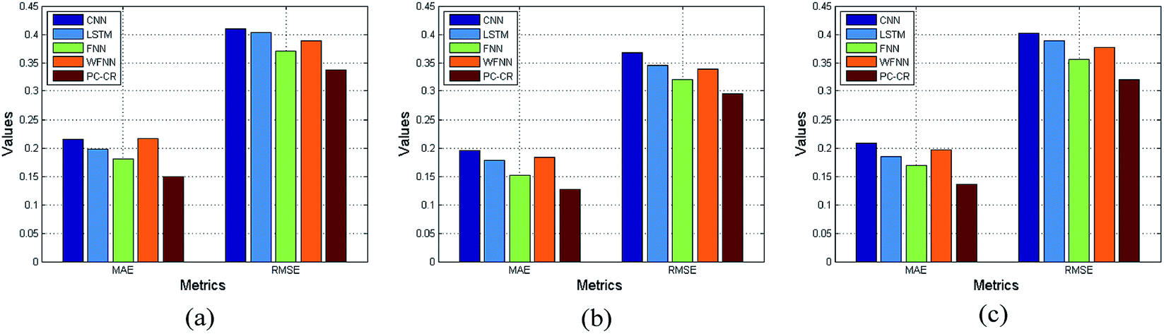
With parameters M, N, λ, and proportion of training set setting to their default values, the learning rate is set to 0.01, 0.005 and 0.001 in order. Fig. 7 and 8 list experimental results of PC-CR and baselines under different values of learning rate. Among, Fig. 7 reveals efficiency of predicted COD, and Fig. 8 reveals efficiency of predicted NH3–N, in which X-axis refers to values of MAE and Y-axis refers to values of RMSE. Each scatter in these two figures represents a “MAE-RMSE” value pair with respect to one method. Obviously, the closer a scatter is to the origin, the better the prediction result is. And two aspects of results can be concluded from them three. Firstly, WFNN performs really worse than other methods. This is because fast operation process leads to the decrease of precision. Secondly, the proposed PC-CR obtained considerable improvement compared with four baselines, regardless of different settings of learning rate. In detail, taking MAE results of predicted COD as an example, the proposed PC-CR is about 5% better than FNN, 8% better than single LSTM, 10% better than CNN, and 13% better than WFNN. The obtainment of such experimental results can be attributed to two aspects of reasons. For one thing, CNN model is employed in this research to deeply extract global features of the WTP at different timestamps, which is the foundation for modelling. For another, RNN model is utilized to capture long-term global features of WTP, which provides a more comprehensive modelling expression. Therefore, this set of experiments preliminarily demonstrate superiority of the combination of CNN and RNN.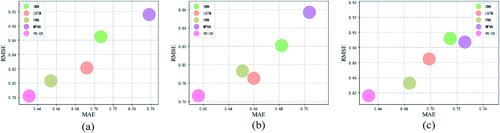 | ||
| Fig. 7 Results of outlet COD under different values of learning rate: (a) 0.01, (b) 0.005 and (c) 0.001. | ||
 | ||
| Fig. 8 Results of outlet NH3–N under different values of learning rate: (a) 0.01, (b) 0.005 and (c) 0.001. | ||
With parameters M, N, λ, and learning rate setting to their default values, the proportion of training data is set to 60%, 70% and 80% in order. Fig. 9 and 10 lists experimental results of PC-CR and baselines under different proportions of training data: 60%, 70% and 80%. It can be also observed from the two figures that performance tendency of the four methods remains relatively stable. Besides, the proposed PC-CR still performs better than baselines under any proportions of training data. In particular, taking RMSE results of predicted NH3–N as an example, the proposed PC-CR is about 10% better than FNN, 12% better than single LSTM, 15% better than WFNN, and 16% better than CNN. Compared with COD prediction, the proposed PC-CR makes greater improvement when it comes to NH3–N prediction. Two possible reasons may be deduced to explain this phenomenon. Firstly, the proposed PC-CR simultaneously considers local feature space and local feature space. Such a comprehensive feature space construction makes it robust to different scenes. Secondly, the proposed PC-CR model was established mainly considering DO as intermediate parameters, and treatment process of ammonia nitrogen is more reliable on DO.
 | ||
| Fig. 9 Results of outlet COD under different proportions of training data: (a) 60%, (b) 70% and (c) 80%. | ||
 | ||
| Fig. 10 Results of outlet NH3–N under different proportions of training data: (a) 60%, (b) 70% and (c) 80%. | ||
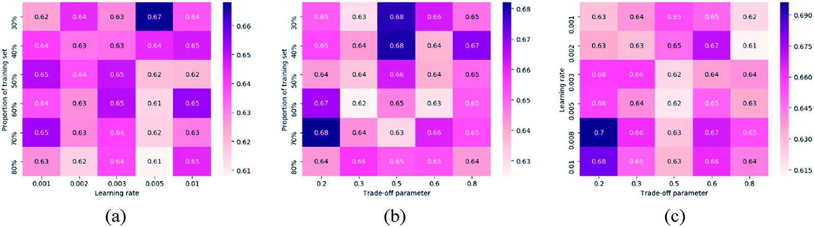
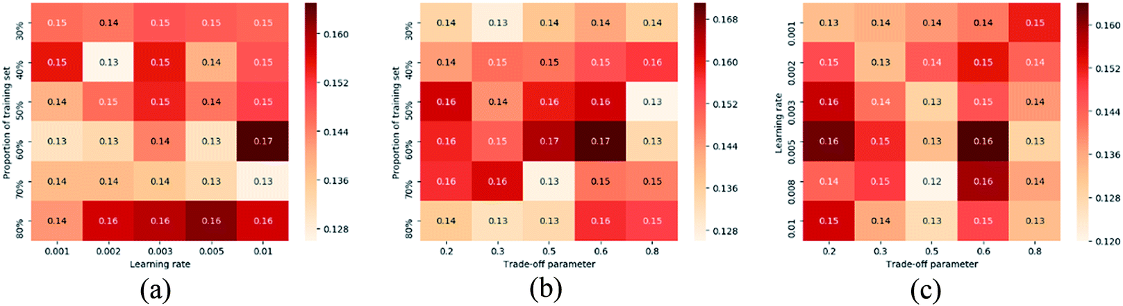
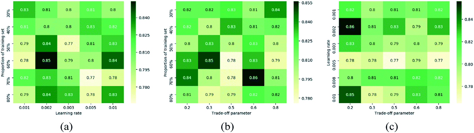
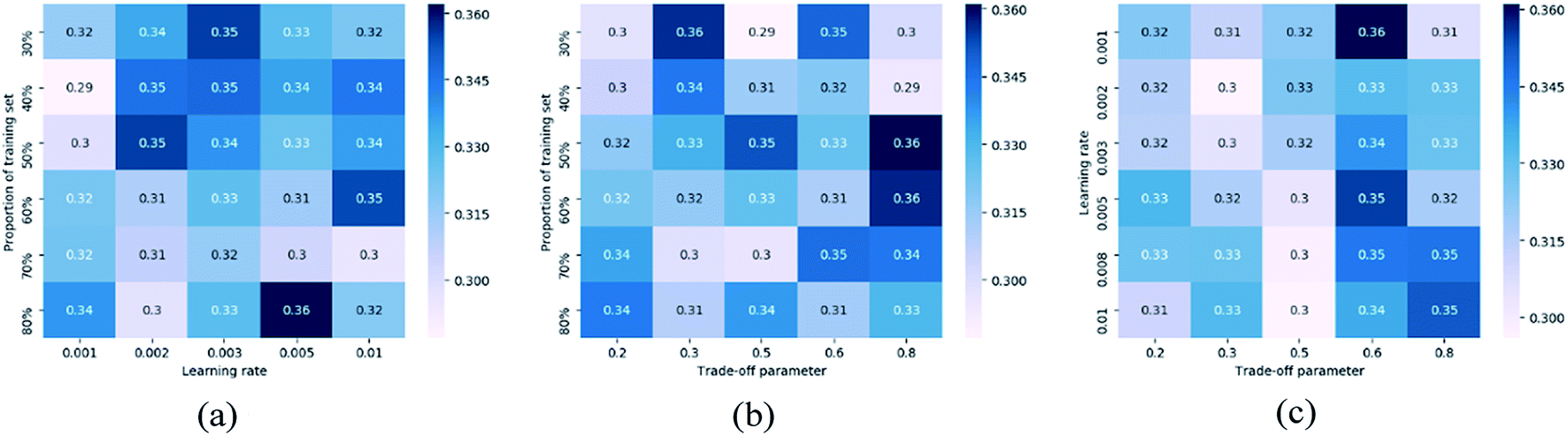
Another set of experiments are conducted to test parameter sensitivity of the proposed PC-CR. In this set of experiments, PC-CR is not compared with any baselines. It is just implemented singly under a number of parameter situations. Fig. 11 and 13 respectively illustrates MAE results and RMSE results of PC-CR with respect to outlet COD under different parameter situations. Fig. 12 and 14 respectively demonstrates MAE results and RMSE results of PC-CR with respect to outlet NH3–N under different parameter situations. All of the four figures have three subfigures, separately corresponding to three types of parameter combination changes: learning rate and proportion of training set, trade-off parameter and proportion of training set, trade-off parameter and learning rate. It can be directly observed from the total twelve subfigures that various experimental results hardly change under different parameter situations, proving proper stability of the proposed PC-CR. It can be deduced from this set of experimental results that PC-CR comprehensively captures both local and global characteristics of the WTP which makes itself not susceptible to changing of parameter situations. Therefore, no matter how the parameter groups change, experimental results never heavily fluctuate and remain relatively stable. To sum up, above experiments prove that the proposed PC-CR possesses both excellent efficiency and stability.
 | ||
| Fig. 11 MAE results of PC-CR with respect to outlet COD under different parameter situations. (a) Changing of learning rate and proportion of training set, (b) changing of trade-off parameter and proportion of training set, (c) changing of trade-off parameter and learning rate. | ||
 | ||
| Fig. 12 MAE results of PC-CR with respect to outlet NH3–N under different parameter situations. (a) Changing of learning rate and proportion of training set, (b) changing of trade-off parameter and proportion of training set, (c) changing of trade-off parameter and learning rate. | ||
 | ||
| Fig. 13 RMSE results of PC-CR with respect to outlet COD under different parameter situations. (a) Changing of learning rate and proportion of training set, (b) changing of trade-off parameter and proportion of training set, (c) changing of trade-off parameter and learning rate. | ||
 | ||
| Fig. 14 RMSE results of PC-CR with respect to outlet NH3–N under different parameter situations. (a) Changing of learning rate and proportion of training set, (b) changing of trade-off parameter and proportion of training set, (c) changing of trade-off parameter and learning rate. | ||
5. Conclusions
In recent years, predicting results of WTP has been a major concern in academia, which requires excellent modelling scheme for WTP. Conventional biochemical mechanism-driven approaches are highly dependent on complicated and redundant model parameters, resulting in low efficiency. Under such background, data-driven approaches emerged as a promising perspective for this issue. However, existing data-driven approaches for this purpose focused on modelling of the WTP at independent timestamps, neglecting sequential characteristics of timestamps during long-term treatment process. To deal with the challenge, this research simultaneously leverages local features of each independent timestamp and global sequential features of the WTP. Thus, a novel prediction and control framework named PC-CR is proposed in this paper. Firstly, CNN model is utilized to automatically extract local features of each independent timestamp in the WTP and make them encoded. Next, RNN model is employed to represent global sequential features of the WTP on the basis of local feature encoding. Finally, we conduct a large amount of experiments to verify efficiency and stability of the proposed PC-CR.Conflicts of interest
There are no conflicts of interest to declare.Acknowledgements
This research was supported by National Key Research & Development Program of China (2016YFE0205600), Innovation Group of New Technologies for Industrial Pollution Control of Chongqing Education Commission (CXQT19023), Scientific Research Foundation of Chongqing Technology and Business University (ZDPTTD201917, KFJJ2018060, 1952027), and Chongqing Natural Science Foundation of China (cstc2019jcyj-msxmX0747).References
- S. O. Ganiyu, M. Zhou and C. A. Martínez-Huitle, Appl. Catal., B, 2018, 235, 103–129 CrossRef.
- M. Aslam and J. Kim, Environ. Sci. Pollut. Res., 2019, 26, 1170–1180 CrossRef PubMed.
- A. E. Burakov, E. V. Galunin, I. V. Burakova, A. E. Kucherova, S. Agarwal, A. G. Tkachev and V. K. Gupta, Ecotoxicol. Environ. Saf., 2018, 148, 702–712 CrossRef PubMed.
- N. H. Tran, M. Reinhard and K. Y. H. Gin, Water Res., 2018, 133, 182–207 CrossRef PubMed.
- M. Gągol, A. Przyjazny and G. Boczkaj, Chem. Eng. J., 2018, 338, 599–627 CrossRef.
- A. Wyrwicka and M. Urbaniak, Sci. Total Environ., 2018, 615, 882–894 CrossRef PubMed.
- J. Wang, H. Yang, G. Qi, X. Liu, X. Gao and Y. Shen, RSC Adv., 2019, 9, 1967–1975 RSC.
- J. H. Wang, H. Y. Li, Y. P. Chen, S. Y. Liu, P. Yan, Y. Shen, J. S. Guo and F. Fang, Environ. Sci. Pollut. Res., 2018, 25, 9797–9805 CrossRef CAS PubMed.
- J. H. Wang, H. Y. Li, Y. P. Chen, Y. Dong, X. X. Wang, J. S. Guo, Y. Shen, P. Yan, T. F. Ma, X. Q. Sun, F. Fang and J. Wang, Environ. Pollut., 2018, 229, 199–209 CrossRef.
- G. Crini and E. Lichtfouse, Environ. Chem. Lett., 2019, 17, 145–155 CrossRef CAS.
- P. Krzeminski, M. C. Tomei, P. Karaolia, A. Langenhoff, C. M. R. Almeida, E. Felis, F. Gritten, H. R. Andersen, T. Fernandes, C. M. Manaia, L. Rizzo and D. Fatta-Kassinos, Sci. Total Environ., 2019, 648, 1052–1081 CrossRef CAS.
- X. Huang, R. Wang, T. Jiao, G. Zou, F. Zhan, J. Yin, L. Zhang, J. Zhou and Q. Peng, ACS Omega, 2019, 4, 1897–1906 CrossRef CAS.
- D. B. Miklos, C. Remy, M. Jekel, K. G. Linden, J. E. Drewes and U. Hübner, Water Res., 2018, 139, 118–131 CrossRef.
- C. A. Martínez-Huitle and M. Panizza, Curr. Opin. Electrochem., 2018, 11, 62–71 CrossRef.
- S. Wong, N. Ngadi, I. M. Inuwa and O. Hassan, J. Cleaner Prod., 2018, 175, 361–375 CrossRef.
- M. Bourgin, B. Beck, M. Boehler, E. Borowska, J. Fleiner, E. Salhi, R. Teichler, U. von Gunten, H. Siegrist and C. S. McArdell, Water Res., 2018, 129, 486–498 CrossRef.
- M. Salgot and M. Folch, Current Opinion in Environmental Science & Health, 2018, 2, 64–74 Search PubMed.
- P. S. Goh and A. F. Ismail, Desalination, 2018, 434, 60–80 CrossRef.
- J. Mo, Q. Yang, N. Zhang, W. Zhang, Y. Zheng and Z. Zhang, J. Environ. Manage., 2018, 227, 395–405 CrossRef.
- C. M. Manaia, J. Rocha, N. Scaccia N, R. Marano, E. Radu, F. Biancullo, F. Cerqueira, G. Fortunato, I. C. Iakovides, I. Zammit, I. Kampouris, I. Vaz-Moreira and O. C. Nunes, Environ. Int., 2018, 115, 312–324 CrossRef.
- L. Kang, H. L. Du, X. Du, H. T. Wang, W. L. Ma and M. L. Wang, Desalin. Water Treat., 2018, 125, 296–301 CrossRef.
- T. Ahmad T and M. Danish, J. Environ. Manage., 2018, 206, 330–348 CrossRef PubMed.
- R. Liu, B. Yang, E. Zio and X. Chen, Mech. Syst. Signal Process., 2018, 108, 33–47 CrossRef.
- A. Hosny, C. Parmar, J. Quackenbush, L. H. Schwartz and H. J. W. L. Aerts, Nat. Rev. Cancer, 2018, 18, 500–510 CrossRef.
- I. Kavakiotis, O. Tsave, A. Salifoglou, N. Maglaveras, I. Vlahavas and I. Chouvarda, Comput. Struct. Biotechnol. J., 2017, 15, 104–116 CrossRef.
- Z. Guo, W. Zeng, H. Wang and Y. Shen, IEEE Access, 2019, 7, 24852–24864 Search PubMed.
- Z. Guo, C. Tang, H. Tang, Y. Fu and W. Niu, IEEE Access, 2018, 6, 5865–5878 Search PubMed.
- Z. Guo, C. Tang, W. Niu, Y. Fu, H. Xia, T. Wu and H. Tang, IEEE Access, 2017, 5, 15529–15541 Search PubMed.
- M. Krueger, H. Luo, S. X. Ding, S. Dominic and S. Yin, IFAC-PapersOnLine, 2015, 48, 627–632 CrossRef.
- H. Rahimi, Z. Kavosi, P. Shojaei and E. Kharazmi, Journal of Health Management & Informatics, 2017, 4, 17–24 Search PubMed.
- W. Shao and X. Tian, Chem. Eng. Res. Des., 2015, 95, 113–132 CrossRef.
- K. Sridevi, E. Sivaraman and P. Mullai, Bioresour. Technol., 2014, 165, 233–240 CrossRef.
- E. B. Hassen and A. M. Asmare, Journal of Environmental Treatment Techniques, 2018, 6, 15–25 Search PubMed.
- M. Sadeghassadi, C. J. B. Macnab, B. Gopaluni and D. Westwick, Comput. Chem. Eng., 2018, 115, 150–160 CrossRef.
- T. Yang, W. Qiu, Y. Ma, C. Mohammed and L. Zhang, Neurocomputing, 2014, 136, 88–95 CrossRef.
- J. Ruan, X. Chen, M. Huang and T. Zhang, J. Environ. Sci. Health, Part A: Toxic/Hazard. Subst. Environ. Eng., 2017, 52, 7–14 CrossRef.
- J. F. Qiao, Y. Hou, L. Zhang and H. G. Han, Neurocomputing, 2018, 275, 383–393 CrossRef.
- H. Zhou, CIESC J., 2017, 68, 1516–1524 Search PubMed.
- H. G. Han, L. Zhang, H. X. Liu and J. F. Qiao, Appl. Soft Comput., 2018, 67, 467–478 CrossRef.
- H. Loussifi, K. Nouri and N. B. Braiek, Commun. Nonlinear Sci. Numer. Simul., 2016, 32, 10–30 CrossRef.
- M. Huang, D. Tian, H. Liu, C. Zhang, X. Yi, J. Cai, J. Ruan, T. Zhang, S. Kong and G. Ying, Complexity, 2018, 2018, 1–11 Search PubMed.
- Q. Cong and W. Yu, Measurement, 2018, 124, 436–446 CrossRef.
- H. Choi, K. Cho and Y. Bengio, Neurocomputing, 2018, 284, 171–176 CrossRef.
- Z. Dong, Z. Zhang, Y. Dong and X. Huang, Energy, 2018, 151, 116–125 CrossRef.
- X. Peng, C. Lu, Z. Yi and H. Tang, IEEE Trans. Neural Netw. Learn. Syst., 2016, 29, 218–224 Search PubMed.
- R. Al-Jawfi, Int. Arab J. Inf. Technol., 2009, 6, 304–309 Search PubMed.
- B. Cortez, B. Carrera, Y. J. Kim and J. Y. Jung, Expert Syst. Appl., 2018, 97, 315–324 Search PubMed.
- F. Hoseini, A. Shahbahrami and P. Bayat, J. Digit. Imaging, 2019, 32, 105–115 CrossRef.
| This journal is © The Royal Society of Chemistry 2020 |