
 Open Access Article
 This Open Access Article is licensed under a
 Creative Commons Attribution 3.0 Unported Licence
The interplay among gas, liquid and solid interactions determines the stability of surface nanobubbles†
Marco
Tortora
 a,
Simone
Meloni
*ab,
Beng Hau
Tan
cd,
Alberto
Giacomello
a,
Claus-Dieter
Ohl
e and
Carlo Massimo
Casciola
a
a,
Simone
Meloni
*ab,
Beng Hau
Tan
cd,
Alberto
Giacomello
a,
Claus-Dieter
Ohl
e and
Carlo Massimo
Casciola
a
aDipartimento di Ingegneria Meccanica e Aerospaziale, Università di Roma La Sapienza, Via Eudossiana 18, 00184 Roma, Italy. E-mail: simone.meloni@unife.it
bDipartimento di Scienze Chimiche e Farmaceutiche (DipSCF), Università degli Studi di Ferrara (Unife), Via Luigi Borsari 46, I-44121, Ferrara, Italy
cLow Energy Electronic Systems, Singapore-MIT Alliance for Research and Technology, 1 Create Way, 138602 Singapore
dSchool of Mechanical and Aerospace Engineering, Nanyang Technological University, 50 Nanyang Avenue, 639798 Singapore
eDepartment for Soft Matter, Institute of Physics, Otto-von-Guericke University Magdeburg, 39106 Magdeburg, Germany
First published on 10th November 2020
Abstract
Surface nanobubbles are gaseous domains found at immersed substrates, whose remarkable persistence is still not fully understood. Recently, it has been observed that the formation of nanobubbles is often associated with a local high gas oversaturation at the liquid–solid interface. Tan, An and Ohl have postulated the existence of an effective potential attracting the dissolved gas to the substrate and producing a local oversaturation within 1 nm from it that can stabilize nanobubbles by preventing outgassing in the region where gas flow would be maximum. It is this effective solid–gas potential – which is not the intrinsic, mechanical interaction between solid and gas atoms – its dependence on chemical and physical characteristics of the substrate, gas and liquid, that controls the stability and the other characteristics of surface nanobubbles. Here, we perform free energy atomistic calculations to determine, for the first time, the effective solid–gas interaction that allows us to identify the molecular origin of the stability and other properties of surface nanobubbles. By combining the Tan–An–Ohl model and the present results, we provide a comprehensive theoretical framework allowing, among others, the interpretation of recent unexplained experimental results, such as the stability of surface nanobubbles in degassed liquids, the very high gas concentration in the liquid surrounding nanobubbles, and nanobubble instability in organic solvents with high gas solubility.
1 Introduction
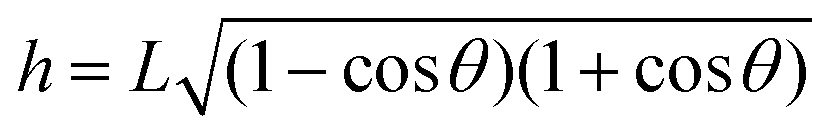
Surface nanobubbles are spherical-cap gas bubbles attached to immersed substrates1,2 (Fig. 1A). They are noted for their counter-intuitive properties, foremost of all their puzzling longevity. Despite numerous efforts over the years, no single model for their stability is widely accepted and able to yield a comprehensive explanation of all their properties.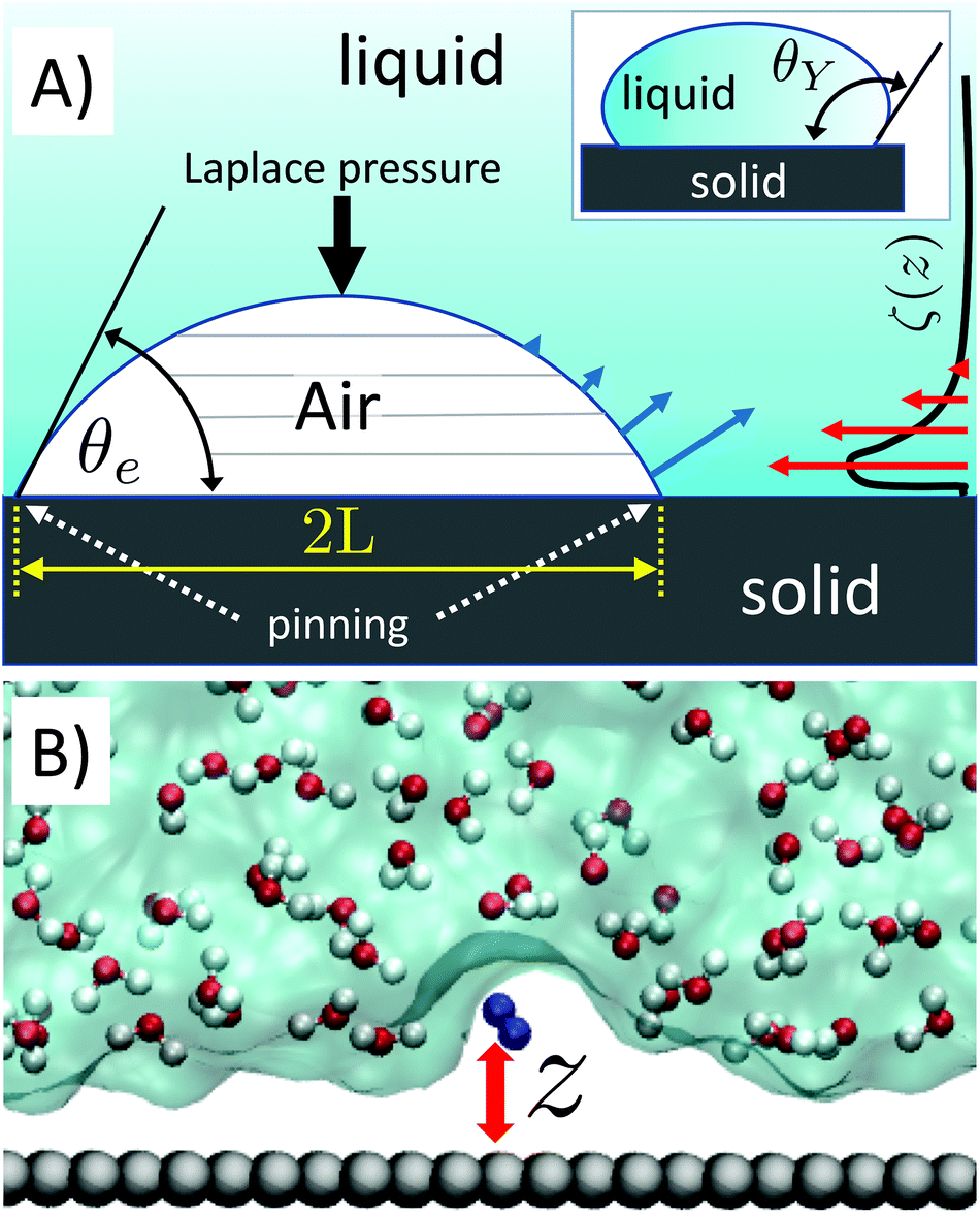 | ||
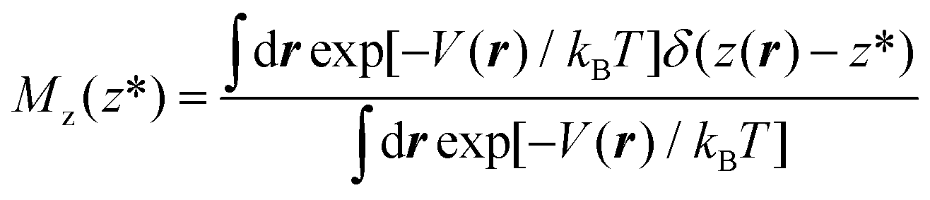
| Fig. 1 (A) Sketch of a nanobubble pinned at a solid surface forming a gas side equilibrium contact angle θe. Due to the small radius of curvature of the bubble and the corresponding large Laplace pressure, estimated to be several atmospheres, a rapid outgassing and, eventually, dissolution of the bubble is expected. The gas outflow (blue arrows, referring to an entire slice) is maximum at the bottom of the bubble, where the liquid/gas surface per bubble slice (horizontal gray lines) is maximum. This intuitively justifies why a large local gas oversaturation within ∼1–2 nm from the surface is efficient at stabilizing nanobubbles: large local oversaturation near the bottom of the nanobubble (red arrows) can balance the gas outflow in the region where it is maximum. In the inset is shown the Young contact angle, θY, the angle formed by the tangent to a liquid droplet at contact point with the surface. (B) Snapshot of a portion of the computational sample. Grey spheres represent carbon atoms of the graphite-like slab, the blue dumbbell N2 and the white and red spheres connected by rod water molecules. The surface enclosing the volume occupied by H2O is also shown. | ||
The fundamental challenge in rationalizing the stability of nanobubbles is well illustrated by the early theoretical calculations of Epstein and Plesset,3 which indicate that spherical bubbles can never achieve stationarity—they either grow catastrophically or dissolve into bulk liquid in a subsecond timescale due to their small size and high curvature. Recently, this difficulty has been overcome by the insight that the contact line of surface nanobubbles may be pinned at nanoscale surface heterogeneities, thus modifying their diffusive dynamics such that they can attain a stable equilibrium when the bulk liquid is oversaturated with gas.4,5 Here, oversaturation is defined as ζ = c∞/csat − 1, where c∞ is the dissolved gas concentration in the bulk liquid and csat is the saturation concentration. Unfortunately, the pinning-oversaturation model cannot be a definitive explanation of the long-term stability of surface nanobubbles. The model requires that ζ > 0, i.e. that gas concentration in the bulk liquid is higher than the saturation value, which is contradicted by the well-established experimental observation of surface nanobubbles in equilibrated open systems (ζ = 0),6 and even under undersaturated conditions (ζ < 0).7–9 Indeed, results reported in ref. 8 led the authors to conclude that “the pinning mechanism alone cannot explain the long-term stability of surface nanobubbles”.
In parallel to theoretical progress, numerous simulation studies have been performed to unveil the mechanistic processes governing the stability of surface nanobubbles.10–12 Although these studies were successful at upholding the importance of contact line pinning to stability, they gave a limited contribution in identifying other key elements to achieve nanobubble stability. Indeed, perhaps influenced by the theoretical hypothesis that nanobubbles are stable only under oversaturated conditions,4,5 but in contrast with experimental evidence,6–9 these works focused only on ζ ≥ 0 conditions. Moreover, standard molecular dynamics techniques adopted in these pioneering studies allow to span a limited timescale, typically few tens of nanoseconds, 11–12 orders of magnitude shorter than the experimentally reported lifetime of nanobubbles, hours to days. This limits the predictive power of these simulations. To cope with these long timescales, special simulation techniques are needed,13,14 some of which have been adopted in the present study.
To resolve the difficulties of the pinning-oversaturation model, Tan, An and Ohl15,16 suggested that an attractive effective potential ϕ of depth ∼1kBT (kB is the Boltzmann's constant and T is the temperature) exists between the substrate and gas molecules, which leads to the formation of a localized gas-oversaturated layer at the surface. ϕ would rationalize the existence of a permanent local oversaturation sustaining surface nanobubbles, while relaxing the unrealistic requirement that the bulk water is indefinitely oversaturated with gas. Combined with pinning, local oversaturation can explain the stability of nanobubbles: (i) pinning prevents the shrinking of their footprint and (ii) local oversaturation counteracts the loss of gas from nanobubbles driven by their high Laplace pressure associated with their small curvature. In the original article, it was shown that a gas-rich water layer of ∼1–2 nm at the liquid/solid interface would be sufficient to stabilize nanobubbles. This is possible because at the bottom of nanobubbles, where slices of the spherical cap have the largest area, the gas exchange is more intense (Fig. 1A). Thus, a local oversaturation in this region can effectively counteract the gas outflux. A number of recent experiments have shown that, indeed, one can produce a large local gas oversaturation at the solid/water interface17,18 and when the oversaturation reaches a critical value, of the order of ζ ∼150–250, nanobubbles are formed.19–21 Among the others, Zhou et al. have performed near-edge X-ray absorption fine structure experiments showing a large gas oversaturation in the liquid surrounding nanobubbles.18 Overall, these results call for a new comprehensive microscopic theory addressing the open questions concerning the stability of nanobubbles in a broader range of experimental conditions and their relationship with the possible existence of a permanent local oversaturation.
The stability of surface nanobubbles in water is not their only unique characteristic. Although stable in water, surface nanobubbles are unstable in selected protic (e.g. ethanol22) and aprotic liquids (organic solvents23). Moreover, surface nanobubbles present small contact angles, well below their equilibrium value, that changes significantly, well above the experimental accuracy, among experiments performed under the same nominal conditions (same solid, liquid, gas, degree of oversaturation ζ and temperature).1 Finally, surface nanobubbles exhibit a remarkable resilience to harsh conditions, such as the near complete degassing of the liquid hosting them.8
The TAO model alone does not provide a direct answer to these questions. Indeed, a key conclusion of the TAO model is that the question “what determines the stability of nanobubbles?” must be recast into “what determines the existence of a suitably attractive effective solid–gas potential ϕ?”. The form and strength of ϕ, which depends on the nature of the solid, liquid and gas species, determines the properties of nanobubbles summarized above. However, within the TAO model, the effective potential ϕ is an input, i.e., it must be obtained from an independent source. By combining the TAO model and the effective potential ϕ, determined here from atomistic simulations – and its dependence on the chemical and physical characteristics of the solid–liquid–gas three phase system – one obtains (i) a comprehensive theory of surface nanobubbles and (ii) a multiscale model with quantitative predictive capabilities.
Here, the form, strength and range of the effective potential is determined using restrained molecular dynamics (RMD), a simulation technique introduced in 2006 by Maragliano and Vanden-Eijnden13,24 extending and simplifying previously well established approaches, e.g. the Blue-Moon ensemble.25,26 This leads us to estimate the local gas oversaturation of the liquid near the substrate and the stability and contact angle of surface nanobubbles hosted in this environment. For solids immersed in water, our results reveal, for the first time, the existence of a potential well of few kBTs at subnanometric distances from the wall, capable of attracting dissolved gases to the substrate, thus endorsing the viability of local oversaturation as a stabilization mechanism for surface nanobubbles in this liquid. By a systematic variation of the liquid–gas–solid interactions, type of liquid and solid our simulations provide a mechanistic understanding of a number of counterintuitive, previously unexplained, phenomena. For example, we were able to explain, within a unified framework, the large variability of nanobubbles’ contact angle at highly ordered pyrolytic graphite immersed in water,1 why the contact angle of nanobubbles shows a minor dependence on the chemical nature of the immersed solid (see ref. 27 and references cited therein), why surface nanobubbles are preferentially formed on hydrophobic substrates28 but survive also on hydrophilic ones,29 the tolerance of nanobubbles to gas undersaturation of water8 as well as their instability in aprotic solvents.23 Furthermore, we were able to pinpoint how the chemical and physical characteristics of the solid, liquid and gas species contribute to the stability or instability of nanobubbles.
2 Computational methods
2.1 Theoretical background
In this work, we use restrained molecular dynamics, RMD, to compute the (Landau) free energy profile as a function of the distance of the center of mass of N2 or O2 from a graphite-like surface, z. This free energy is the microscopic analogue of the effective potential ϕ. We remark that the (Landau) free energy is different from the intrinsic interaction potential between N2 and the solid, i.e. the force field; for example, the free energy embodies the effect of the liquid intervening between the solid and the gas molecule on the interaction potential, which is a key aspect in determining the stability and instability of nanobubbles in different liquids.In statistical mechanics, any thermodynamic potential is related to the logarithm of a suitable probability density function in the relevant ensemble. In the present case, the relevant probability density function is Mz(z*), the probability density that the center of mass of N2 (or O2), the function z(rN2,s) of the atomic positions of nitrogen (or oxygen) and surface atoms rN2,s is at a distance z* from the graphite slab, regardless of the position of all the other atoms in the system. For the sake of simply of notation, in the following, we will write the distance between the center of mass of N2 and the solid surface as a function of the (3N dimensional) atomic position vector r. In terms of the ensemble distribution m(r), Mz(z*) reads:
 | (1) |
One can associate a thermodynamic potential to Mz(z*), here the (Landau) free energy (see, e.g., ref. 30 and 31).
G(z*) = −kBT![[thin space (1/6-em)]](https://www.rsc.org/images/entities/char_2009.gif) logMz(z*) logMz(z*) | (2) |
One notices that this definition has the properties of usual thermodynamics potentials: G(z*) has a minimum at the stable state, i.e. in correspondence with the maximum of the probability density function, and is expressed in energy units. One may notice that this definition is consistent with the definition of the Boltzmann entropy, apart the sign, which is opposite, consistently with the properties of entropy to be maximum at the stable state, and for the units of measure, which is energy divided by temperature for entropy. Finally, it can be shown that ΔG = G(z2*) − G(z1*) between two states can be expressed as the reversible work operated by a generalized force to move the system from z1* to z2*,31 which is consistent with the definition of free energies in thermodynamics.
To compute Mz(z*) – hence G(z*) – in atomistic simulations one can in principle run a long molecular dynamics trajectory and determine the histogram of z along it; this histogram is a discrete approximation of Mz(z*) from which one can compute the free energy viaeqn (2). However, it is well known that this approach is computationally inefficient (see, e.g., ref. 30 and references cited therein). The key problem is that if the effective interaction is attractive, the molecule spends most of the time near the surface, if it is repulsive, the molecule is all the simulation far from the substrate; in both cases, it is impossible to collect statistics at all relevant z values within the timescale accessible by atomistic simulations (maximum hundreds of ns).
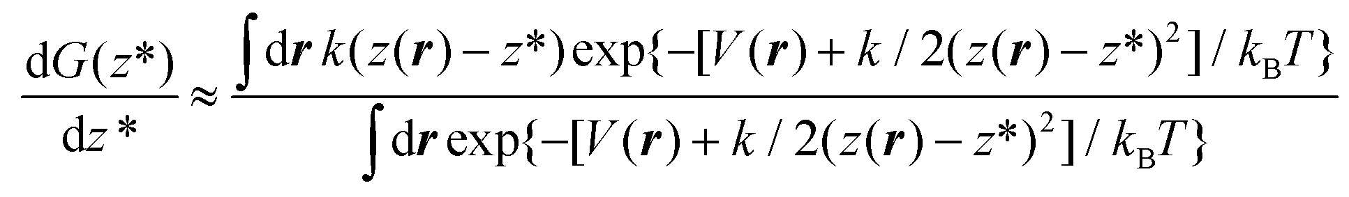
To overcome this problem, we use RMD,13,24,32 in which one introduces a controlled bias forcing the system to explore configurations, in which the distance z(r) of a gas molecule from the substrate is fixed at the value z*.‡ In other words, within RMD, one forces the system to visit only those configurations consistent with the condition z(r) = z*. As we will show in the following, this allows us to efficiently estimate the derivative of the free energy G(z*), i.e. dG(z*)/dz*, which can then be numerically integrated on z* to obtain the entire profile of the thermodynamic potential as a function of the distance of N2 from the graphite slab. The estimation of dG(z*)/dz* can be expressed as a local average of a suitable observable on the hyperplane z(r) = z* and restrained MD can be used to compute this average.
In more detail, consider the (Landau) free energy of eqn (2) and for the sake of simplicity assume that the ensemble is canonical, hence m(r) = exp[−V(r)/kBT]/∫drexp[−V(r)/kBT], where V(r) is the (physical) interacting potential, the so-called force field. We remark that the arguments developed below can be straightforwardly extended to other ensembles, e.g. isothermal–isobaric. Within the canonical ensemble, the probability density function of eqn ((1) reads):
 | (3) |
 | (4) |
In eqn (4), one can replace the Dirac delta functions with a smooth Gaussian approximation, δ(z(r) − z*) ∼ gk(z − z*) =
  exp[−k/(2kBT)(z
 − z*)2]. kBT/k is the variance of the Gaussian function, the parameter determining its width and the accuracy of the approximation to the corresponding Dirac delta function. The reason to express the variance of the gaussian by the apparently more complex form kBT/k will be clear shortly. Here, we just remark that T, the temperature, is determined by the experimental conditions (T = 300 K, in our case); k is the only parameter of the RMD method, whose suitable value can be determined as explained in the following. By replacing δ(z(r) − z*) with gk(z(r) − z*) in eqn (4), one can obtain an explicit, though approximated, formula for the derivative of the free energy:
 | (5) |
Eqn (5) shows that, within the Gaussian approximation of the Dirac delta function, the derivative of the free energy can be computed as the expectation value of k(z(r) − z*) over the canonical ensemble of a system driven by the so-called augmented potential V(r) + k/2(z(r) − z*)2. In practice, one computes dG(z*)/dz* at the current value of z* by averaging the observable k(z(r) − z*) along the trajectory of a constant number of particles/volume/temperature molecular dynamics, restrained by the potential k/2(z(r) − z*)2. The operation is repeated for several values of z* in the relevant range, here between 0.4 nm and 1.6 nm every 0.02 nm, then the so-obtained dG(z*)/dz* is numerically integrated by the trapezoidal rule.
The suitable value of k is determined by studying the convergence of the approximate dG(z*)/dz*, eqn (5), with increasing k at a set of z* values. In the present case, k = 0.7 kcal mol−1 Å−2.
2.2 Simulation details
The sample we considered in our simulation consists of a 5-layer thick slab of graphite with an ABAB pattern34 in contact with TIP4P/2005 water35 containing a single N2 or O2 molecule. The molecule interacts with the surface and the liquid through a Lennard-Jones (LJ) potential v(rij) = 4εαβ((σαβ/rij)12 − (σαβ/rij)6), where rij is the distance between an atom of the molecule and one of the surface or water. εαβ sets the strength of the interaction between atoms of type α and β and σαβ the corresponding range. The values of εαβ and σhaβ are determined using the Lorentz–Berthelot combination rules: σαβ = 1/2(σα + σβ) and , where σx and εx are the parameters characterizing two atoms of the same species. For the purely repulsive gas–solid potential, we use the so-called Weeks–Chandler–Andersen potential. This potential is obtained from the N2-graphite one by cutting off the LJ potential at rij = 21/6σαβ, i.e. at its minimum, and keeping it constant for rij > 21/6σαβ. For σx and εx, we used the values reported in Table 1. To model a liquid with a higher air solubility, we used a value of εNO three times larger than that used for water. The relationship between force field parameters and gas solubility is explained in the ESI†.
Consistently with the TIP4P/2005 model,35 interaction between graphite and water is modeled by a modified LJ potential, v(rij) = 4εCO((σCO/rij)12 − c(σCO/rij)6), in which the attractive term is scaled by a factor c.36c can be tuned to control the hydrophobicity of the surface. In practice, we compute the Young contact angle θY formed by a cylindrical droplet deposited on the graphite slab (Fig. ESI1†) for 26 values of c in the range 0.5–0.75 with a spacing of 0.01. Over this range, we observed a linear relationship between θY and c (Fig. ESI2†); thus, from the fitting of the θY–c pairs, we estimate the values of c corresponding to the Young contact angles of water used in free energy calculations: 70°, 80°, 90°, 100° and 110°.
Once again, consistent with the TIP4P/2005 model,35 the gas/water interaction is also modeled by a LJ potential in which the parameters are obtained by literature data via the Lorentz–Berthelot combination rules.
To mimick aprotic organic solvents, we use a LJ liquid with the same parameters of oxygen in the TIP4P/2005 water model. Solid–liquid interaction is modeled using the same modified LJ potential used for water, in which the “c” parameter has been optimized to obtain the same Young contact angle values used for H2O. For the liquid–gas interaction, we maintained the values used for water, hence the same affinity between the gas and the liquid.
The approximation of considering a single gas molecule dissolved in the liquid, which neglects possible interactions among gas molecules, is justified by the low solubility of air in water. In fact, as we will show in sec. 3, even considering the highest computed local oversaturation and the bulk liquid in equilibrium with air (no degassing), the highest value of local molar fraction is ∼0.02, corresponding to one molecule of gas every ∼50 molecules of water. Considering the N–O pair correlation function of N2 in water (Fig. ESI3†), 50 neighbor water molecules per N2 corresponds to an ∼1.4 nm average distance between pairs of gas molecules, which is beyond the distance at which N–N interactions are negligible, ∼1 nm.
3. Results and discussion
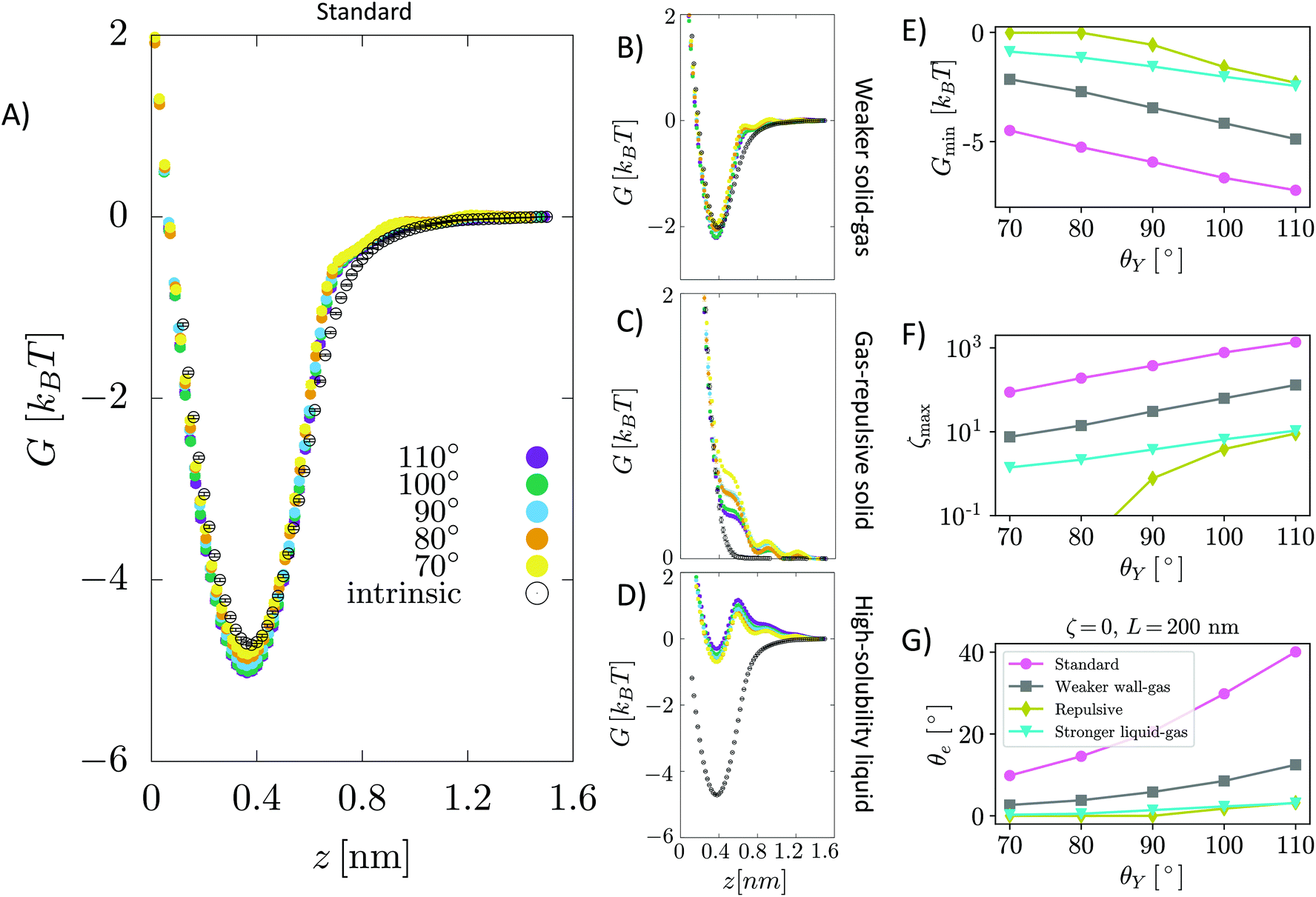
We investigate the attraction of dissolved gas by a solid wall in a simulation sample consisting of a 5-layer-thick slab (∼1.5 nm) of graphite assembled in an ABAB pattern,34 in contact with liquid (TIP4P/200535) water. We then introduce either a single N2 or O2 molecule (see Fig. 1B) in water; note that these two species alone account for 99% of the composition of air. The choice to simulate a single gas molecule is justified by the fact that, even at the largest local over saturations, the average distance between pairs of gas molecules is larger than their interaction length (see sec. 2). The N and O atoms of the nitrogen and oxygen molecules interact with the carbon atoms of the substrate and the oxygen atoms of the water molecules via the Lennard-Jones (LJ) potential, whose parameters have been obtained from literature data (see sec. Simulation details). We consider several levels of hydrophobicity of the substrate, characterized by the following values of the Young contact angle: θY = 70°, 80°, 90°, 100° and 110°. This is achieved by modifying the graphite/water LJ interaction. This system is designed to model highly ordered pyrolytic graphite (HOPG) immersed in water, typically used in surface nanobubble experiments. Details of the computational setup and parameters used in the calculations are given in the Simulation details section.We use the system described above to calculate the effective potential attracting gas molecules to an immersed surface. This, using the TAO model to connect atomistic results with experimental data (see below), allows to develop a microscopic theory of the stability of surface nanobubbles. We compute the (Landau) free energy G between a nitrogen/oxygen molecule and the graphite-like slab as a function of z, the separation between the molecule's center of mass and the substrate (Fig. 1B). G(z) is the microscopic equivalent of the interaction potential, ϕ(z), responsible for the local oversaturation at the core of the TAO model. G(z) is computed using restrained molecular dynamics, RMD, which is described in detail in the Theoretical background section.
Our calculations show that between N2 and graphite immersed in water there is a substantial potential well (Fig. 2A) generating a large localized oversaturation within 1 nm of the substrate (see the inset). This large localized oversaturation is consistent with recent experimental results.18 More difficult is the comparison with computational results available in the literature, which also predicts a large oversaturation at the solid–liquid interfaces.17,41 In fact, in these works, the authors use a different computational approach consisting of preparing a sample with a very high gas oversaturation and determining the gas local oversaturation profile as a function of the distance from the surface. In our case, in constrast, thanks to the use of RMD to compute the free energy, we can consider more realistic bulk oversaturation conditions.
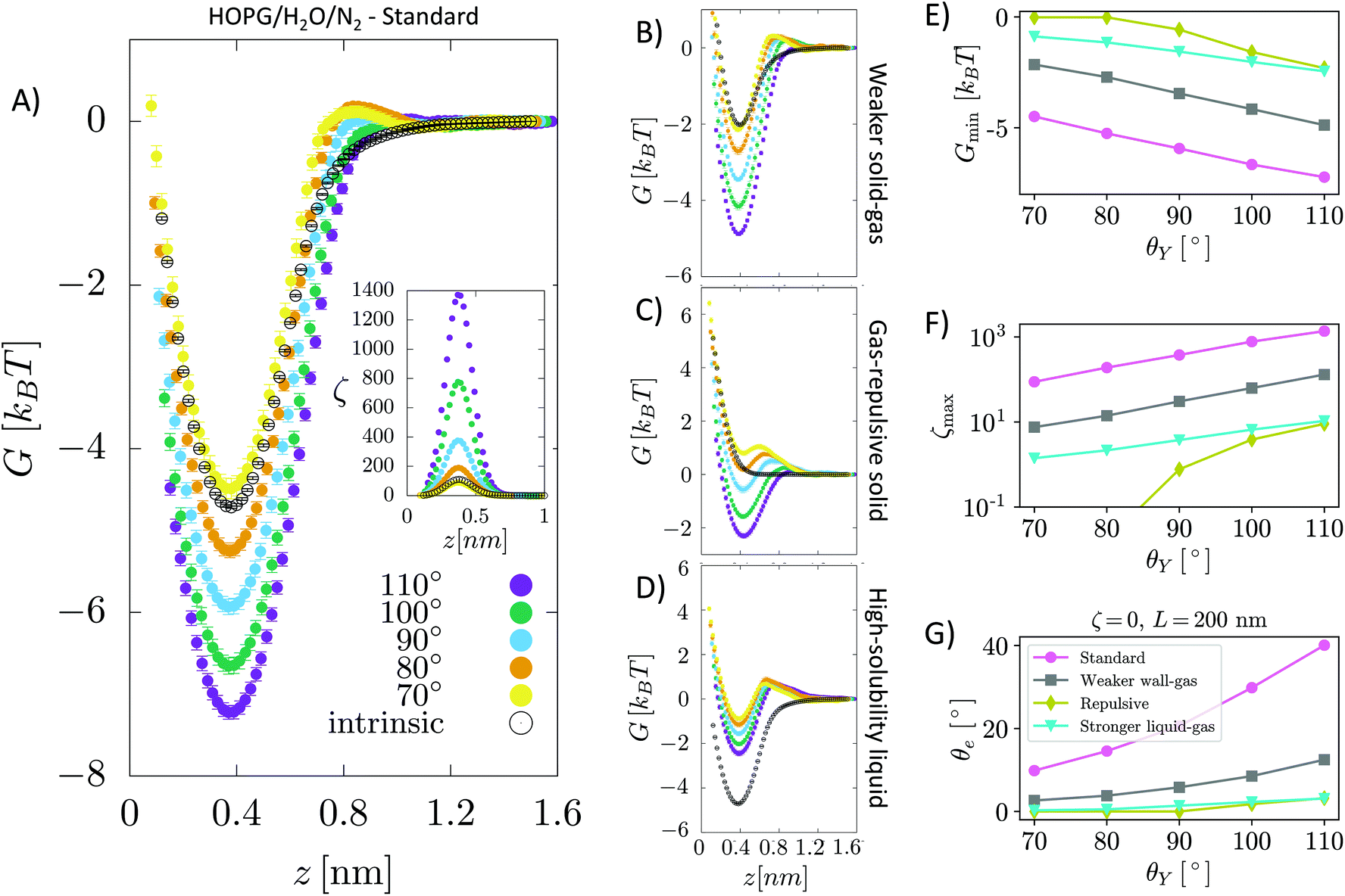 | ||
| Fig. 2 (A–D) Free energy G(z) of an N2 molecule in water on a graphite-like slab as a function of the distance from the surface. G(z) is reported for several values of the Young contact angle of the liquid θY, solid–gas intrinsic interaction and liquid–gas interaction strength. As a reference, we report also G(z) in the absence of water, i.e. considering only graphite–N2 interactions (empty circles). Panel (A) shows the results of the sample modeling HOPG/H2O/N2, also denoted as the standard; (B) for a sample with a weaker solid–gas interaction; (C) for the case of a purely gas-repulsive surface;40 (D) for a highly soluble gas. The error bars, barely visible in the figure, have size comparable to that of symbols represented in the panels (see the ESI† for a discussion on the method adopted to compute the error in free energy calculations). In the inset, the local oversaturation ζ(z) for the HOPG/H2O/N2 sample is reported. (E–G) Minimum of the free energy Gmin, maximum of the local oversaturation ζmax and equilibrium contact angle of the nanobubbles θe as a function of the hydrophobicity of the surface θY for the four systems. θe is estimated from eqn (6), considering a nanobubble of L = 200 nm radius in a saturated liquid ζbulk = 0. | ||
In general, the free energy exhibits two properties that are common for all values of the Young contact angle investigated. Firstly, G(z) presents a characteristic minimum at ∼0.4 nm from the surface, with a well depth ranging from 4 to 7.5kBT; the well depth Gmin increases with θY (Fig. 2E), i.e., the more hydrophobic the surface, the more it attracts nitrogen dissolved in water (Fig. 2F). Secondly, the free energy reaches its bulk value over a distance of ∼1 nm. We remark that the range of this effective interaction is not determined by the cutoff of the solid–gas intrinsic interaction (only), which is 1.6 nm, but by the complex interplay between solid–gas, solid–liquid and liquid–gas interactions. This will be shown more in detail in the following. The free energy profile also presents additional features, such as a tiny maximum at ∼0.7 nm that becomes more pronounced for more hydrophilic surfaces. The origin of the peculiar shape of G(z) and its dependence on the characteristics of the solid, liquid and gas will be discussed in detail in a forthcoming article.
It should be stressed that the general features of G(z) are not specific to nitrogen. In the ESI,† we present the results of analogous calculations for O2 dissolved in water, illustrating the similarities of the free energy profiles of nitrogen and oxygen (Fig. ESI4†).
Next, we connect atomistic results to experimental data, namely nanobubbles’ contact angles, using the TAO model, in which the free energy curves of Fig. 2 represent the key input (see the ESI† for a brief summary of the TAO model). The model is summarized by eqn (6), which is the condition that must be satisfied for the gas flow at the liquid–gas interface of the bubble to be zero (stationary) in the pinning-local oversaturation theory:
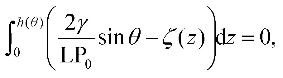 | (6) |
Here, the local oversaturation is (inset of Fig. 2A):
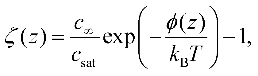 | (7) |
 . The solution of eqn (6) is the nanobubble contact angle θ for which the net gas flux in and out of the bubble is zero, i.e., the equilibrium contact angle θe. Fig. 2G shows that the effective solid–gas attraction of Fig. 2A is sufficient to produce stable nanobubbles with equilibrium contact angles within the typical experimental range.1 In particular, consistent with recent experimental findings,22,23,29,42,43 our results show that nanobubbles can persist on nominally hydrophilic substrates.
The present results allow us to address two puzzling questions about nanobubbles at HOPG in water: (i) why is the contact angle much lower than the value one could predict from θY (i.e., θe≠ 180° − θY, considering the opposite convention for the Young and nanobubble contact angles)? (ii) why is the experimental value of the contact angle of nanobubbles at HOPG scarcely reproducible? We remark that the TAO model is necessary but not sufficient to address this and the other questions discussed in the following. To answer these questions, one needs the results obtained in this work for the first time, i.e., the calculation from atomistic simulations of the effective solid–gas potential ϕ(z). In fact, the TAO model provides a connection between the microscopic properties of the system, namely G(z), and its macroscopic characteristics, the nanobubbles contact angle θe, but the TAO model itself does not provide any estimation of the effective solid–gas interaction. Concerning the first question, our calculations show that given the strength of the solid/gas interaction and the typical Young contact angle of HOPG, which is slightly hydrophilic, one can achieve a local oversaturation that can compensate the outflow gas from the bubble only when θe is rather small, 20° or lower (Fig. 2G). This is, indeed, a combined effect of the pinning and local oversaturation model. Concerning the limited reproducibility of θe values, it is known that the variation among data reported by different research groups exceeds the experimental accuracy of contact angle measurements.1 To answer this question, one has to take into account that the preparation history of the HOPG substrate influences the effective affinity between water and graphite. In particular, the Young contact angle θY of water on HOPG depends sensitively on how quickly the liquid is deposited onto the substrate. When deposited on freshly cleaved graphite, a droplet of water has θY ∼70°, but upon prolonged exposure to ambient air this value substantially increases to 80–90°.23,44Fig. 2G (pink dots) shows that if we take this variation in θY into account, the estimated values of θe are in the range 5 ≤ θe ≤ 20°, spanning an interval matching that reported in the authoritative review by Lohse and Zhang.1 In summary, for HOPG substrates, the history of the experimental sample affects its hydrophobicity that, in turn, changes the effective HOPG/air attraction and, through it, θe.
Can the effective air attraction explain the survival of surface nanobubbles under (bulk) non-oversaturated conditions, i.e., in open (ζ = 0),6 or degassed systems (ζ < 0)?7–9 In Fig. 3A, we report the degree of undersaturation ζ* = c∞*/csat − 1 (<0) that nanobubbles can withstand before their equilibrium contact angle becomes negligible according to eqn (6). A negative value of ζ* means that the gas concentration in the liquid bulk,  , is lower than the saturation value, csat. ζ* is a convenient measure of the tolerance of nanobubbles to degassing. The equilibrium contact angle decreases monotonically with decreasing air concentration in the bulk liquid16 until it reaches a critical value ζ* at which θe = 0° (Fig. 3B). One notices that for the HOPG/water/air, nanobubbles can sustain any level of degassing (blue line). Of course, the ζ* = 0 limit must be understood in the sense that the liquid still contains enough air that can accumulate at the surface to counteract nanobubble degassing. Under these conditions, the bulk oversaturation ζ is negligible with respect to saturation conditions ζ = 1, virtually corresponding to complete degassing. Although the precise value of ζ* might be critically affected by the limited accuracy of the empirical potentials used in our simulations, our general conclusions are consistent with the results reported in a very recent article8 showing that nanobubbles resisted to the highest level of degassing the authors were able to achieve (∼80% of air dissolved in water was removed). As mentioned in the Introduction, their results led Qian et al. to conclude that the pinning-supersaturation mechanism is insufficient at explaining the long-term stability of surface nanobubbles. The present work allows the reconciliation of experiments and theory, adding the missing ingredient – local gas supersaturation at the wall – to the pinning model, which can explain the stability of nanobubbles under degassing conditions.
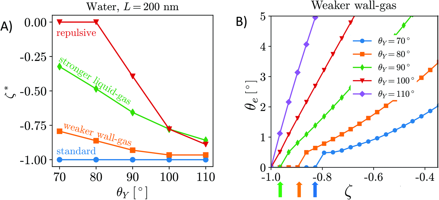 | ||
| Fig. 3 (A) Tolerance of nanobubbles to degassing measured as critical undersaturation ζ*. (B) The equilibrium contact angle vs. oversaturation, showing that θe decreases monotonically with decreasing air concentration in the bulk liquid16 until at ζ* it reaches θe = 0°. In particular, in panel B, we report the values of the equilibrium contact angle vs. ζ for the case of the weaker solid–gas interaction. Each curve corresponds to a different value of the surface hydrophobicity, θY. The colored arrows indicate the ζ* values. | ||
We remark that the TAO model and the present calculations do not allow the complete determination of the lifetime of nanobubbles. For example, the TAO model assumes contact line pinning but, indeed, the triple line can depin (see, e.g., ref. 45) and, as a consequence, nanobubbles can possibly be destabilized. Indeed, the relationship between contact line pinning and nanobubble lifetime has been experimentally confirmed (see, e.g., ref. 9). The characteristic times of contact line depinning and other processes determining the lifetime of nanobubbles are beyond the aim of the TAO model and of the present work. The theoretical determination of the timescale of these processes requires the use of other advanced simulation techniques.13,46,47
3.1 Effect of solid–liquid–gas interactions on the stability of nanobubbles
In the following, through a systematic variation of the solid–liquid–gas interactions, we investigate (i) the dependence of the stability of nanobubbles on the characteristics of the three phases and (ii) we show that our theory can explain a number of counterintuitive properties observed in experiments.In addition to the standard sample modeling HOPG in water, we considered two alternative cases: first, a weaker solid–gas interaction, half the strength of HOPG/N2 (Fig. 2B), and second, a purely repulsive solid–gas interaction, via the so-called Weeks–Chandler–Andersen potential40 (Fig. 2C). The standard case shows that – except for the most hydrophilic case θY = 70° – the presence of water strengthens the effective solid–gas interaction beyond its intrinsic value, i.e. the well of G(z) in the presence of water is deeper than that of a substrate exposed to nitrogen gas only (dashed line in Fig. 2A). We stress that this does not mean that the density of gas at the substrate is higher in the liquid than in the nanobubble as G(z) is computed taking as a reference the value in the liquid and the pure gas, respectively; our results indicate that there might be a different gas enrichment at the substrate, which for the HOPG/H2O/N2 system at θY > 70° is higher in the liquid than in nanobubbles. Generally speaking, the higher the Young contact angle, the stronger the effective solid–gas attraction, which results in larger nanobubble contact angles (Fig. 2G). A similar trend is also observed for the weaker (halved) intrinsic solid–gas interaction (Fig. 2B), where the free energy is attractive for all Young contact angles. Comparing results in panels A and B of Fig. 2, one notices that the main effect of a weaker solid–gas interaction is a shift of all curves toward less attractive values, with the corresponding reduction in the local oversaturation (Fig. 2F) and nanobubbles’ contact angles (Fig. 2G). The weaker solid–gas attraction reduces the tolerance to undersaturation (Fig. 3), which, however, remains high.
It is worth remarking that despite the significant reduction in the solid–gas intrinsic interaction, the nanobubble still presents a non-negligible contact angle also at hydrophilic substrates. This is due to the enhancement in the effective gas attraction associated with the presence of water and explains the relative independence of the nanobubble contact angle on the chemical nature of the substrate (see ref. 27 and references cited therein). It is worth stressing that the TAO model alone is not sufficient to predict the dependence of nanobubbles’ contact angle on the strength of the intrinsic solid–gas interaction, i.e. on the chemical nature of the solid and gas. In fact, the effective potential G(z) determining θe critically depends on the presence of the liquid, and this dependence is non-trivial, as we will show in the following. Indeed, in most theoretical models of nanobubble stability, the liquid is considered an inert medium, while here, for the first time, we show that the liquid plays a critical and active role in the properties of surface nanobubbles.
It is remarkable that also in the case of a purely repulsive intrinsic solid–gas interaction, the presence of water may bring an effective attraction, provided that the surface is hydrophobic (Fig. 2C). Of course, in this case the effective solid–gas attraction is weaker and the nanobubble contact angle is reduced to a few degrees, see Fig. 2G. Nanobubbles with such small contact angles, corresponding to a thickness of 5–10 nm for a nanobubble of 400 nm footprint (radius L = 200 nm), are more difficult to detect experimentally. Also, in this case, the tolerance to degassing is reduced, but nanobubbles at purely gas-repulsive surfaces can withstand ζ < 0 provided that the substrate is hydrophobic (θY ≥ 90°).
The case of the purely repulsive intrinsic solid–gas interaction illustrates the relevance of the gas–liquid interaction in determining the effective potential acting on the gas. In fact, one notices that G(z) is non-negligible well beyond the distance of N2 from the surface, where the intrinsic solid–gas interaction is zero. To explain the effect of the liquid and the value of its Young contact angle on the free energy, we propose that the effective solid–gas interaction is due to the balance between its intrinsic strength, i.e. the strength in the absence of liquid (dashed line in Fig. 2A–C), and the gas solubility. The intuitive argument behind this hypothesis is that if the gas is insoluble, i.e. if hosting it in the liquid is energetically disfavored, it will preferentially accumulate at the solid/water interface, where the hydrogen bond network of the liquid is already compromised and the energetic cost of insertion of a molecule is reduced. The more hydrophobic the surface, the less energetically expensive it is to replace a molecule of water at the solid/water interface with one of N2 (or O2). Moreover, due to the depletion of liquids at the interface with solids (see, e.g., ref. 48), G(z) reaches its plateau value at a z distance where the liquid has fully recovered its bulk density. In fact, for larger distances from the wall, the gas molecule is embedded in a liquid environment that is independent on the position z and the effective interaction potential becomes flat. This explains why the range of G(z) is longer than that of the purely repulsive intrinsic solid–gas interaction, as the range of the effective potential is determined by the width of the depletion zone. The effect of gas solubility in the liquid is discussed in more detail below.
Summarizing, we found that nanobubbles with a contact angle up to ∼10° can be formed also at surfaces with a weak intrinsic solid–gas attraction; even purely gas-repulsive surfaces can produce stable nanobubbles, although their small contact angle might prevent their experimental identification. For surfaces with low gas attraction, the stabilization of nanobubbles requires a complementary high hydrophobicity, which enhances the strength of the effective solid–gas attraction. In contrast, relatively strong intrinsic solid–gas interactions (few kBTs) can lead to stable nanobubbles also at hydrophilic surfaces. By revealing the key and active role of the liquid in determining the strength of the effective solid–gas interaction, our simulations allow the explanation of the experimental observation that in water surface the contact angle of nanobubbles seemingly ceases to be dependent on the chemical nature of the substrate, typically falling in the range 5° ≤ θe ≤ 20°.1
The effect of gas solubility on the stability of surface nanobubbles has been observed in experiments. Surface nanobubbles are known to be very stable in water and are insensitive even to the addition of high concentrations of acids, bases or salts. However, a notable exception to their reputed ‘superstability’ is that, when surface nanobubbles in water have their liquid replaced with ethanol, they destabilize and dissolve.22 Systematic experiments have further shown that the surface coverage of nanobubbles incubated in water–ethanol mixtures monotonously drops to zero as the mole fraction of the alcohol is progressively increased from 0 to 20%. Note that ethanol, which, similar to water, presents strong hydrogen bonding among its molecules as confirmed by a relatively high boiling point (∼79 °C), has double the gas solubility of water; thus, consistently with experiments, our theory predicts that surface nanobubbles are unstable in a liquid with an air solubility as high as that in ethanol across the entire range of θY, which is again consistent with experiments.
3.2. Nanobubbles in aprotic liquids
The fact that experiments are nearly exclusively performed in water has, over time, raised questions about possible specific properties of this liquid in stabilizing surface nanobubbles. Can surface nanobubbles exist in non-aqueous liquids? Is hydrogen bonding responsible for the persistence of surface nanobubbles in water? These questions will be addressed in this section. An influential experimental study by An et al.23 positively answers both questions. The authors used solvent exchange various non-aqueous liquids to nucleate surface nanobubbles on HOPG. They found surface nanobubbles to exist in protic solvents but not in aprotic ones, leading them to propose that a hydrogen bonding network is necessary for the stability of surface nanobubbles.To isolate the effect of the hydrogen bonding in our simulations, we replaced water with a (mono-atomic) Lennard-Jones liquid with the same LJ parameters as in the TIP4P/2005 model.35 It is worth recalling that the TIP4P/2005 model is characterized by two contributions: (i) the electrostatic interactions among point charges centered on H and O atoms, which result in the formation of hydrogen bonding among H2O molecules reproducing the typical tetrahedral structure of water and (ii) the non-directional interaction among LJ centers positioned slightly off of oxygen atom, determining the “size” of the molecule. Thus, by replacing the TIP4P/2005 water model with the corresponding LJ allowed us to effectively investigate the effect of hydrogen bonding. To make the comparison stringent, the solid–liquid interaction is tuned to form the same Young contact angle as for water on HOPG considered above: 70° < θY < 110°. Liquid–gas and solid–gas interactions are the same as that in the water case (see sec. Simulation details for additional information).50 Thus, the only difference with previous simulations is the absence of hydrogen bonding within the liquid. This setup is not meant to model any specific solid/liquid/gas system; here, we exploit the flexibility of simulations to model systems with ad hoc characteristics to identify the role of hydrogen bonding to stabilize nanobubbles.
Fig. 4A, B and C show G(z) for a surface immersed in the aprotic, LJ liquid when the solid–gas intrinsic interaction is standard, weakened (halved) and purely repulsive. These panels are equivalent to the corresponding panels of Fig. 2 for water. Our results show that strong attractive effective solid–gas interactions may still be present but this is due to the intrinsic characteristics of the solid–gas pair: aprotic solvents do not enhance this interaction. Thus, in an aprotic liquid, one cannot obtain stable nanobubbles at purely gas-repulsive surfaces even if they are highly solvophobic. The present results are consistent with the explicit molecular dynamics simulations by Maheshwari et al.,11 which show that a pinned surface nanobubble in a classic LJ liquid could be stable, albeit in the original article these conclusions have been drawn only for a short timescale of 30 ns.
 | ||
| Fig. 4 The same panels as in Fig. 2 for a graphite surface immersed in an aprotic, Lennard-Jones liquid. In particular, in panels A–D, we show G(z) for several values θY for HOPG/LJ/N2, for the halved solid–gas interaction, for the gas-repulsive surface and for a highly gas-soluble liquid, respectively. Except for the purely repulsive surface, one notices that the effect of an aprotic, structureless, liquid on the effective solid/gas interaction is negligible. In other words, the aprotic liquid does not enhance the intrinsic solid–gas attraction. Panels E–G show the values of the minimum of the free energy Gmin, maximum of the oversaturation ζmax and equilibrium nanobubbles contact angle θe for the cases shown in the A–D panels. θe in panel G is computed from eqn (6) considering a nanobubble of L = 200 nm radius in a saturated liquid ζbulk = 0. | ||
The fact that aprotic solvents do not deepen the solid–gas well seems related to the lack of directional intermolecular interactions, which make the liquid–liquid cohesion stronger in the protic case. Thus, at a variance with water and other protic liquids, there is no or only a minor energetic gain to move the solute gas from the bulk to the solid/liquid interface, and one expects a lower local oversaturation. In the case of purely repulsive surfaces, the presence of an aprotic liquid increases the repulsion because there is an energetic penalty to have an interaction with a gas molecule rather than a (or more) liquid particle, and this is not balanced by the penalty to move the gas molecule in the liquid bulk, like in the case of hydrogen bonded liquids. In short, at a variance with water, an aprotic liquid does not enhance the intrinsic solid–gas attraction, which must be strong enough to stabilize nanobubbles.
Another effect one has to take into account is that non-polar gases often have a higher solubility in aprotic liquids. In the previous section, we have already shown that a higher gas solubility reduces the effective solid–gas attraction, which destabilizes nanobubbles. To prove that the same concept holds also in the case of aprotic liquids, the above calculations were repeated for the case of a stronger liquid–gas interaction. As for the case of water, we increased the liquid–gas interaction strength by a factor 3. Also in this case, a higher solubility weakens the effective solid–gas attraction; moreover, since hydrophobicity plays a minor role in the case of aprotic liquids, here the solid–gas effective interaction is too weak to stabilize nanobubbles over the entire range of θY considered.
The principle we have just identified, that gas solubility is key at determining the stability of nanobubbles, provides a theoretical framework to explain recent experimental results on aprotic liquids. Consider, for example, dimethyl sulfoxide (DMSO); nitrogen has a solubility in DMSO that is about one order of magnitude higher than that in water51 and An et al.23 have shown that nanobubbles are unstable in the former liquid. Similarly, propylene carbonate (PC), another aprotic liquid that An et al. have shown to be unable to form nanobubbles, has a nitrogen solubility which is more than twice that of water.52,53 Additionally, both do not form hydrogen bonds and have a lower contact angle at HOPG than water (DMSO θY = 45°, PC θY = 31°, water ∼70°), which further weakens the effective gas–solid interaction.
Summarizing, our results show a more subtle picture of stability of nanobubbles than previously hypothesized: aprotic liquids can still form attractive wells for the dissolved gas and hence form stable nanobubbles of sizable contact angle (Fig. 4G), provided that the solid–gas interaction is strong enough. However, another effect competes, and might overcome the strength of solid–gas attraction, i.e. the gas solubility in the liquid, which for air is usually higher in aprotic solvents.
4 Conclusions
In this work, we have computed the effective interaction potential between a solvated gas molecule and a planar substrate, with a view towards understanding how the effective, liquid-mediated solid–gas interaction affects the stability and other properties of surface nanobubbles. These calculations explain why surface nanobubbles have small contact angles, obtaining theoretical θe values in quantitative agreement with experimental results. Moreover, our calculations allow the explanation why nanobubbles are stable in water on a surprisingly wide variety of substrates with disparate hydrophobicities and gas affinities, under undersaturated conditions, and yet also catastrophically destabilize in organic solvents. The ability of our calculations, in conjunction with the TAO model, to simultaneously account for the vast majority of experimental observations on surface nanobubbles suggests that it effectively and comprehensively captures the chemistry and physics of the stability of surface nanobubbles and its dependence on the chemical nature of the solid, liquid and gas species.Conflicts of interest
There are no conflicts to declare.Acknowledgements
The research received funding from the European Research Council under the European Union's Seventh Framework Programme (FP7/2007-2013)/ERC grant agreement no. 339446 and under European Union's Horizon 2020 Research and Innovation Programme grant agreement no. 803213. S. M. acknowledges financial support from the Sapienza University of Rome, grant no. RG11715C81D4F43C, and from the project HPC-EUROPA3 (INFRAIA-2016-1-730897), with the support of the EC Research Innovation Action under the H2020 Programme’, grant no. HPC174LQMN. B. H. T. acknowledges financial support from the SMART Fellowship. C. D. O. acknowledges support from the Joint Research Programme of the National Natural Science Foundation of China (11861131005) and the Deutsche Forschungsgemeinschaft (OH 75/3-1). The authors acknowledge PRACE for awarding access to resource MARCONI based in Italy at Casalecchio di Reno.References
- D. Lohse and X. Zhang, Rev. Mod. Phys., 2015, 87, 981 CrossRef CAS.
- M. Alheshibri, J. Qian, M. Jehannin and V. S. Craig, Langmuir, 2016, 32, 11086–11100 CrossRef CAS.
- P. S. Epstein and M. S. Plesset, J. Chem. Phys., 1950, 18, 1505–1509 CrossRef CAS.
- D. Lohse and X. Zhang, Phys. Rev. E: Stat., Nonlinear, Soft Matter Phys., 2015, 91, 031003 CrossRef.
- C. U. Chan, M. Arora and C.-D. Ohl, Langmuir, 2015, 31, 7041–7046 CrossRef CAS.
- H. An, B. H. Tan, Q. Zeng and C.-D. Ohl, Langmuir, 2016, 32, 11212–11220 CrossRef CAS.
- X. H. Zhang, G. Li, N. Maeda and J. Hu, Langmuir, 2006, 22, 9238–9243 CrossRef CAS.
- J. Qian, V. S. Craig and M. Jehannin, Langmuir, 2018, 35, 718–728 CrossRef.
- X. Zhang, D. Y. Chan, D. Wang and N. Maeda, Langmuir, 2013, 29, 1017–1023 CrossRef CAS.
- Y. Liu and X. Zhang, J. Chem. Phys., 2014, 141, 134702 CrossRef.
- S. Maheshwari, M. van der Hoef, X. Zhang and D. Lohse, Langmuir, 2016, 32, 11116–11122 CrossRef CAS.
- J. H. Weijs, J. H. Snoeijer and D. Lohse, Phys. Rev. Lett., 2012, 108, 104501 CrossRef.
- S. Bonella, S. Meloni and G. Ciccotti, Eur. Phys. J. B, 2012, 85, 1–19 CrossRef.
- S. Meloni, A. Giacomello and C. M. Casciola, J. Chem. Phys., 2016, 145, 211802 CrossRef.
- B. H. Tan, H. An and C.-D. Ohl, Phys. Rev. Lett., 2018, 120, 164502 CrossRef.
- B. H. Tan, H. An and C.-D. Ohl, Phys. Rev. Lett., 2019, 122, 134502 CrossRef CAS.
- W. Chun-Lei, L. Zhao-Xia, L. Jing-Yuan, X. Peng, H. Jun and F. Hai-Ping, Chin. Phys. B, 2008, 17, 2646 CrossRef.
- L. Zhou, X. Wang, H.-J. Shin, J. Wang, R. Tai, X. Zhang, H. Fang, W. Xiao, L. Wang, C. Wang, X. Gao, J. Hu and L. Zhang, J. Am. Chem. Soc., 2020, 142, 5583–5593 CrossRef CAS.
- Q. Chen, H. S. Wiedenroth, S. R. German and H. S. White, J. Am. Chem. Soc., 2015, 137, 12064–12069 CrossRef CAS.
- S. R. German, M. A. Edwards, H. Ren and H. S. White, J. Am. Chem. Soc., 2018, 140, 4047–4053 CrossRef CAS.
- H. Ren, S. R. German, M. A. Edwards, Q. Chen and H. S. White, J. Phys. Chem. Lett., 2017, 8, 2450–2454 CrossRef CAS.
- C. U. Chan and C.-D. Ohl, Phys. Rev. Lett., 2012, 109, 174501 CrossRef.
- H. An, G. Liu, R. Atkin and V. S. J. Craig, ACS Nano, 2015, 9, 7596–7607 CrossRef CAS.
- L. Maragliano and E. Vanden-Eijnden, Chem. Phys. Lett., 2006, 426, 168–175 CrossRef CAS.
- M. Sprik and G. Ciccotti, J. Chem. Phys., 1998, 109, 7737–7744 CrossRef CAS.
- E. Carter, G. Ciccotti, J. T. Hynes and R. Kapral, Chem. Phys. Lett., 1989, 156, 472–477 CrossRef CAS.
- J. R. Seddon and D. Lohse, J. Phys.: Condens. Matter, 2011, 23, 133001 CrossRef.
- L. Wang, X. Wang, L. Wang, J. Hu, C. L. Wang, B. Zhao, X. Zhang, R. Tai, M. He and L. Chen, et al. , Nanoscale, 2017, 9, 1078–1086 RSC.
- C. U. Chan, L. Chen, M. Arora and C.-D. Ohl, Phys. Rev. Lett., 2015, 114, 114505 CrossRef.
- B. Peters, Reaction rate theory and rare events, Elsevier, 2017 Search PubMed.
- G. Stoltz and M. Rousset, et al., Free energy computations: A mathematical perspective, World Scientific, 2010 Search PubMed.
- S. Meloni and G. Ciccotti, Eur. Phys. J. Spec. Top., 2015, 12, 2389–2407 CrossRef.
- E. A. Carter, G. Ciccotti, J. T. Hynes and R. Kapral, Chem. Phys. Lett., 1989, 156, 472–477 CrossRef CAS.
- D. D. L. Chung, J. Mater. Sci., 2002, 37, 1475–1489 CrossRef CAS.
- J. L. Abascal and C. Vega, J. Chem. Phys., 2005, 123, 234505 CrossRef CAS.
- L. Joly, C. Ybert, E. Trizac and L. Bocquet, Phys. Rev. Lett., 2004, 93, 257805 CrossRef.
- J. Walther, R. Jaffe, T. Halicioglu and P. Koumoutsakos, Center for turbulence research: proceedings of the summer program, 2000, pp. 5–20 Search PubMed.
- T. Werder, J. H. Walther, R. Jaffe, T. Halicioglu and P. Koumoutsakos, J. Phys. Chem. B, 2003, 107, 1345–1352 CrossRef CAS.
- J. Jiang and S. I. Sandler, J. Am. Chem. Soc., 2005, 127, 11989–11997 CrossRef CAS.
- J. D. Weeks, D. Chandler and H. C. Andersen, J. Chem. Phys., 1971, 54, 5237–5247 CrossRef CAS.
- S. Wang, L. Zhou, X. Wang, C. Wang, Y. Dong, Y. Zhang, Y. Gao, L. Zhang and J. Hu, Langmuir, 2019, 35, 2498–2505 CrossRef CAS.
- N. Hain, D. Wesner, S. I. Druzhinin and H. Schönherr, Langmuir, 2016, 32, 11155–11163 CrossRef CAS.
- D. Seo, S. R. German, T. L. Mega and W. A. Ducker, J. Phys. Chem. C, 2015, 119, 14262–14266 CAS.
- A. I. Aria, P. R. Kidambi, R. S. Weatherup, L. Xiao, J. A. Williams and S. Hofmann, J. Phys. Chem. C, 2016, 120, 2215–2224 CrossRef CAS.
- A. Murmur, Adv. Colloid Interface Sci., 1994, 50, 121–141 CrossRef.
- A. Giacomello, L. Schimmele and S. Dietrich, Proc. Natl. Acad. Sci. U. S. A., 2016, 113, E262–E271 CrossRef CAS.
- S. Marchio, S. Meloni, A. Giacomello and C. M. Casciola, Nanoscale, 2019, 11, 21458–21470 RSC.
- M. Maccarini, R. Steitz, M. Himmelhaus, J. Fick, S. Tatur, M. Wolff, M. Grunze, J. Janecek and R. Netz, Langmuir, 2007, 23, 598–608 CrossRef CAS.
- E. Wilhelm and R. Battino, J. Chem. Phys., 1971, 55, 4012–4017 CrossRef CAS.
- We remark that in the water case, nitrogen (and oxygen) atoms interacted only with the oxygen atom of water via a LJ interaction. Here, we maintain the same interaction, hence the same affinity between the gas and the liquid.
- R. Battino, T. R. Rettich and T. Tominaga, J. Phys. Chem. Ref. Data, 1984, 13, 563–600 CrossRef CAS.
- A. Kohl and R. Nielsen, Gas purification, Gulf Professional Publishing, Houston, 1997, 1188–1234 Search PubMed.
- V. Baranenko, V. Sysoev, L. Fal'kovskii, V. Kirov, A. Piontkovskii and A. Musienko, Sov. At. Energy, 1990, 68, 162–165 CrossRef.
Footnotes |
| † Electronic supplementary information (ESI) available: Estimation of the free energy error; summary of the local oversaturation theory; relationship between force field parameters and gas solubility; details on contact angle calculations; nitrogen–water pair correlation function; free energy for the HOPG/H2O/O2 system. See DOI: 10.1039/D0NR05859A |
| ‡ Indeed, RMD forces the system to visit atomic configurations almost satisfying the condition z(r) = z*. As explained in the main text, the departure from this condition is determined by the coupling parameter k of the auxiliary potential k/2(z(r) − z*)2 added to the physical interaction potential. Maragliano and Vanden-Eijnden have proven that the estimate of dG(z*)/dz* converges smoothly with k, i.e. one can use a finite value of the coupling parameter to determine the derivative of the mean force within the accuracy of one or few kBTs. On the other hand, releasing the strict condition of the constraint solves the problem of the implicit – and undesired – additional constraint z(r) = 0, which makes the computational determination of dG(z*)/dz* more complex.33 |
| This journal is © The Royal Society of Chemistry 2020 |