
 Open Access Article
 This Open Access Article is licensed under a
 Creative Commons Attribution 3.0 Unported Licence
The optical nanosizer – quantitative size and shape analysis of individual nanoparticles by high-throughput widefield extinction microscopy†
Lukas M.
Payne
 ab,
Wiebke
Albrecht
cd,
Wolfgang
Langbein
*b and
Paola
Borri
a
ab,
Wiebke
Albrecht
cd,
Wolfgang
Langbein
*b and
Paola
Borri
a
aThe Sir Martin Evans Building, School of Biosciences, Cardiff University, Cardiff, Wales, UK
bThe Queen's Buildings, School of Physics and Astronomy, Cardiff University, Cardiff, Wales, UK. E-mail: langbeinww@cardiff.ac.uk
cEMAT, University of Antwerp, Groenenborgerlaan 171, B-2020 Antwerp, Belgium
dNANOlab Center of Excellence, University of Antwerp, Belgium
First published on 8th July 2020
Abstract
Nanoparticles are widely utilised for a range of applications, from catalysis to medicine, requiring accurate knowledge of their size and shape. Current techniques for particle characterisation are either not very accurate or time consuming and expensive. Here we demonstrate a rapid and quantitative method for particle analysis based on measuring the polarisation-resolved optical extinction cross-section of hundreds of individual nanoparticles using wide-field microscopy, and determining the particle size and shape from the optical properties. We show measurements on three samples consisting of nominally spherical gold nanoparticles of 20 nm and 30 nm diameter, and gold nanorods of 30 nm length and 10 nm diameter. Nanoparticle sizes and shapes in three dimensions are deduced from the measured optical cross-sections at different wavelengths and light polarisation, by solving the inverse problem, using an ellipsoid model of the particle polarisability in the dipole limit. The sensitivity of the method depends on the experimental noise and the choice of wavelengths. We show an uncertainty down to about 1 nm in mean diameter, and 10% in aspect ratio when using two or three color channels, for a noise of about 50 nm2 in the measured cross-section. The results are in good agreement with transmission electron microscopy, both 2D projection and tomography, of the same sample batches. Owing to its combination of experimental simplicity, ease of access to statistics over many particles, accuracy, and geometrical particle characterisation in 3D, this “optical nanosizer” method has the potential to become the technique of choice for quality control in next-generation particle manufacturing.
1. Introduction
Nanoparticles (NPs) of various chemical compositions, sizes, shapes, and surface-functionalizations are ubiquitous in modern research and industry, with uses ranging from drug-delivery,1 biomedical imaging2 and sensing,3,4 to catalysis5 and photovoltaics.6 For all these applications, knowledge of the NP size and shape is a key requirement. Notably, many NPs used in the aforementioned fields have dimensions well below the diffraction limit (of about 250 nm) for visible light. This presents a significant challenge for the quantification of the size and shape of individual NPs using optical microscopy.The industry standard for accurate determination of NP sizes and geometry is electron microscopy, particularly transmission electron microscopy (TEM). TEM provides very high resolution, down to atomic detail, owing to the small wavelength of an electron beam, but is complex, expensive, and “low-throughput” in terms of the number of NPs examined in one field of view and corresponding statistics.7 An alternative, non-optical technique to characterize particle size distributions is tunable resistive pulse sensing8–10 (TRPS), which detects the change of the ionic current when a particle passes through a membrane pore. The change in electric resistance is related to the volume, and thus a sizing can be achieved on this premise. The method is high-throughput, accurate, can cover a wide range of particle sizes, and offers the additional benefit of charge and concentration measurement, but is typically limited to NPs larger than about 60 nm, does not provide shape information, and requires calibration before each measurement session.
Centrifugation10,11 techniques measure particle size distributions via sedimentation rates, allowing good determination even with polydisperse samples, and in some cases are capable of resolution down to 1 nm. However, these are inherently ensemble techniques, do not offer shape information, and require or assume a homogeneous particle material density. A related group of methods is field-flow fractionation, which use flow-based elution and separation of particulates. Asymmetric flow field-flow fractionation (AF4),10,12 uses two flow sources to separate and elute particles, and is often combined with dynamic light scattering (DLS) and multi-angle light scattering (MALS). AF4-DLS-MALS10,12,13 has been shown to be a robust particle characterization method even capable of providing some indirect shape information by comparing the geometric (MALS) and hydrodynamic (DLS) radii. The setups can however be costly, requiring of significant expertise and sample species-specific setup to make sure samples properly elute.
Recently, a variant of DLS has been developed, called particle tracking analysis14 (PTA), which observes Brownian motion of single particles over time to determine their hydrodynamic radius. As with DLS, PTA typically has issues for NP sizes below 20 nm due to their weak scattering. Neither DLS nor PTA can provide information on NP shapes.
Notably, it is possible to relate the magnitude of light absorbed and/or scattered by a NP, with its size and shape. In other words, the optical absorption and/or scattering cross-sections, σabs and σsca respectively, or their sum, known as the extinction cross-section, σext, carry information on the NP geometry. σabs can be measured via a technique called photothermal imaging15–17 (PTI), achieving detection of gold nanoparticles (GNP) down to about 1.4 nm.18σext has been measured by spatial modulation microscopy16,19,20 (SMS), with demonstrated detection down to about 2 nm, and GNPs in this size range exhibit σext around 1 nm2. However, both techniques require expensive apparatus, careful calibration, and are slow, being laser-scanning based, implying a limitation on throughput. A more direct absorption measurement technique21,22 employing laser scanning without modulation has demonstrated detection of absorption of single molecules with σext ≈ σabs ≈ 0.1 nm2. However, this method is also slow and not amenable to high-throughput characterization. Darkfield microscopy is used to measure σsca, and can typically detect particles down to about 20 nm size for gold and silver nanospheres or dielectric particles such as polystyrene beads down to about 70 nm size23–25 or nanodiamonds.26 In this case, the limit is most significantly a practical one, as scattering by the target NPs is overwhelmed by scattering of their surroundings (typically dielectric debris). Furthermore, σsca scales as the 6th power of the radius for NPs of dimensions within the dipole approximation, suggesting significant requirements on acquisition time and camera noise properties for particle sizes well below 20 nm.
Ref. 27 presents an on-chip sensing device based on whispering gallery modes (WGM), exhibiting detection and sizing of (non-absorbing) potassium chloride and polystyrene particles from 60 nm to about 200 nm when probing with light close to infrared (wavelength λ = 670 nm). This technique is notably not limited to the spherical assumption, since the signal is related to the polarizability of the NPs, and thus various shape models could be implemented. However, careful fabrication of the WGM resonator is critical. Ref. 28 uses widefield reflection microscopy, exploiting the interference between the scattered light of NPs and the substrate reflection, measured as a function of defocus. GNPs and polystyrene beads of 50–70 nm size were separated and their size determined by a machine learning approach. Differential interference contrast wide-field imaging has been used to determine the orientation of gold nanostars,29 but not their cross-sections.
We have recently shown that a simple transmission based technique using only widefield illumination is capable of simultaneously detecting hundreds of NPs with σext down to 1 nm2, corresponding to a 2 nm GNP.30–32 This procedure is rapid, quantitative and can be augmented using excitation light of varying polarisation direction, to gain information on the NP shape, and of varying wavelength, to gather material and shape-specific spectral properties. It is however not a trivial task to solve the inverse problem, i.e. to derive size and shape parameters from the measurement of σext, especially when treating hundreds of NPs measured simultaneously.
In this paper, we introduce a method solving this inverse problem. We measure σext with a simple wide-field technique on hundreds of individual GNPs, both nominally spherical and rod-shaped, and simulate σext using a semi-analytical model in the dipole limit. We demonstrate that a retrieval of the NP size, shape, and orientation in three dimensions is possible, by fitting the measurements with the model. The accuracy of this “optical nanosizer” is discussed in relation to the measurement parameters, and bench-marked against state-of-the-art TEM and STEM 2D projection and STEM tomography.
2. Method and model
An object in an incident electromagnetic (EM) field will remove and redistribute power from that field resulting in a “shadow” being cast. In the limit of an object much larger than the wavelength λ, the shadow can be approximated by a simple projection of the object's cross-section orthogonal to the propagation direction, hence geometrical optics provides a suitable platform by which to determine the projected physical size and shape of the object. However, diffraction effects dominate for objects whose diameter D is comparable to, or smaller than the wavelength (D < λ), which in the visible wavelength range is the case for a NP. In this diffraction-limited regime, the “shadow” cast by the NP would be imaged as a shape close to the point spread function (PSF) of the imaging system. The exact form depends on the optics involved, the wavelength and polarisation of the incident light, the NP material, size, shape, and the refractive index of the environment. We also note that the PSF is in principle extended, and one needs to consider the area integral of the intensity of the PSF over the plane of projection, to determine the power removed by the particle from the incident field. In practice, one needs to limit integration to a range close to the diffraction limited size in order to control noise and surrounding structure, as we have discussed previously.33 From these measurements, using the incident intensity Iinc, the absorbed power Pabs, and the scattered power Psca, the optical absorption and scattering cross-sections, σabs = Pabs/Iinc and σsca = Psca/Iinc, respectively, can be determined, whose sum is called the extinction cross-section, σext = σabs + σsca = Pext/Iinc. Now, measuring these quantities as a function of wavelength and light polarization, and modelling them, the NP properties such as orientation, size, shape, and material can be inferred.We describe here the model we use to determine the cross-sections σabs, σsca, and σext from the NP properties. We assume the incident field to be a plane wave and a linear optical response of the NP. For NPs much smaller than the wavelength, D/λ ≪ 1, one can disregard the phase difference of the field across the NP, a situation called the Rayleigh regime (or dipole limit). For larger particles, an analytical treatment for spherical particles is given by Mie theory. However, the resulting expressions contain infinite sums, and elliptical particles cannot be treated analytically. Therefore, the present work uses a description in the Rayleigh regime, for which simple analytical expressions exist even for elliptical shapes, given by the Rayleigh–Gans theory.34 This choice is not mandatory, but reduces the numerical effort in the present work, particularly when comparing the model to the measurements of hundreds of NPs. The accuracy of the dipole approximation is evaluated for spherical gold NPs in the ESI section II.D.†
For an ellipsoidal NP, it is useful to choose a Cartesian reference system of unit vectors  , with κ = x′, y′, and z′, in the directions of the NP semi-axes of lengths a, b, and c, which are ordered so that a ≥ b ≥ c. The polarisability of the NP in its reference frame is then given by
 | (1) |
 | (2) |
 . The factors Lj are determined by the geometry of the NP, and given by the analytical expression,
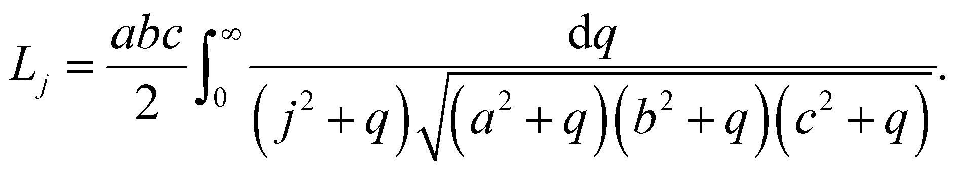 | (3) |
For the general case these integrals must be solved numerically, but closed-form solutions exist when at least two of the semi-axes are identical, i.e. for prolate and oblate spheroids, as well as spheres.35
For metallic NPs, ε1 becomes increasingly negative above the plasma wavelength, resulting in a vanishing real part of the denominator in eqn (2) at a specific wavelength, for which
| ReεNP(λ) = εm(1 − Lj−1), | (4) |
Since a NP can have an arbitrary orientation in the measurement instrument, we need to transform eqn (1) into the measurement frame,34 yielding ![[small alpha, Greek, circumflex]](https://www.rsc.org/images/entities/i_char_e101.gif) . In the NP's reference frame, the polarization induced by a field,
. In the NP's reference frame, the polarization induced by a field,  , incident on an NP with polarisability, ′, is given by
 | (5) |
For the measurement frame, we label the axes of the Cartesian coordinates, ι∈{x, y, z}, with unit vectors  , where
  is along the optical path, and
  ,
,  are spanning the sample plane, as illustrated in Fig. 1. A vector
  in the NP frame is transformed into
  in the measurement frame as,
 | (6) |
![[R with combining circumflex]](https://www.rsc.org/images/entities/i_char_0052_0302.gif) , so that for the NP polarization we have
, so that for the NP polarization we have | (7) |
| = ′T, | (8) |
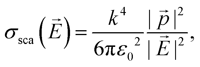
−1, is equal to the transposed matrix T. In general, will therefore have non-zero off-diagonal elements. It can be shown34 that σabs and σsca are given by | (9) |
 | (10) |
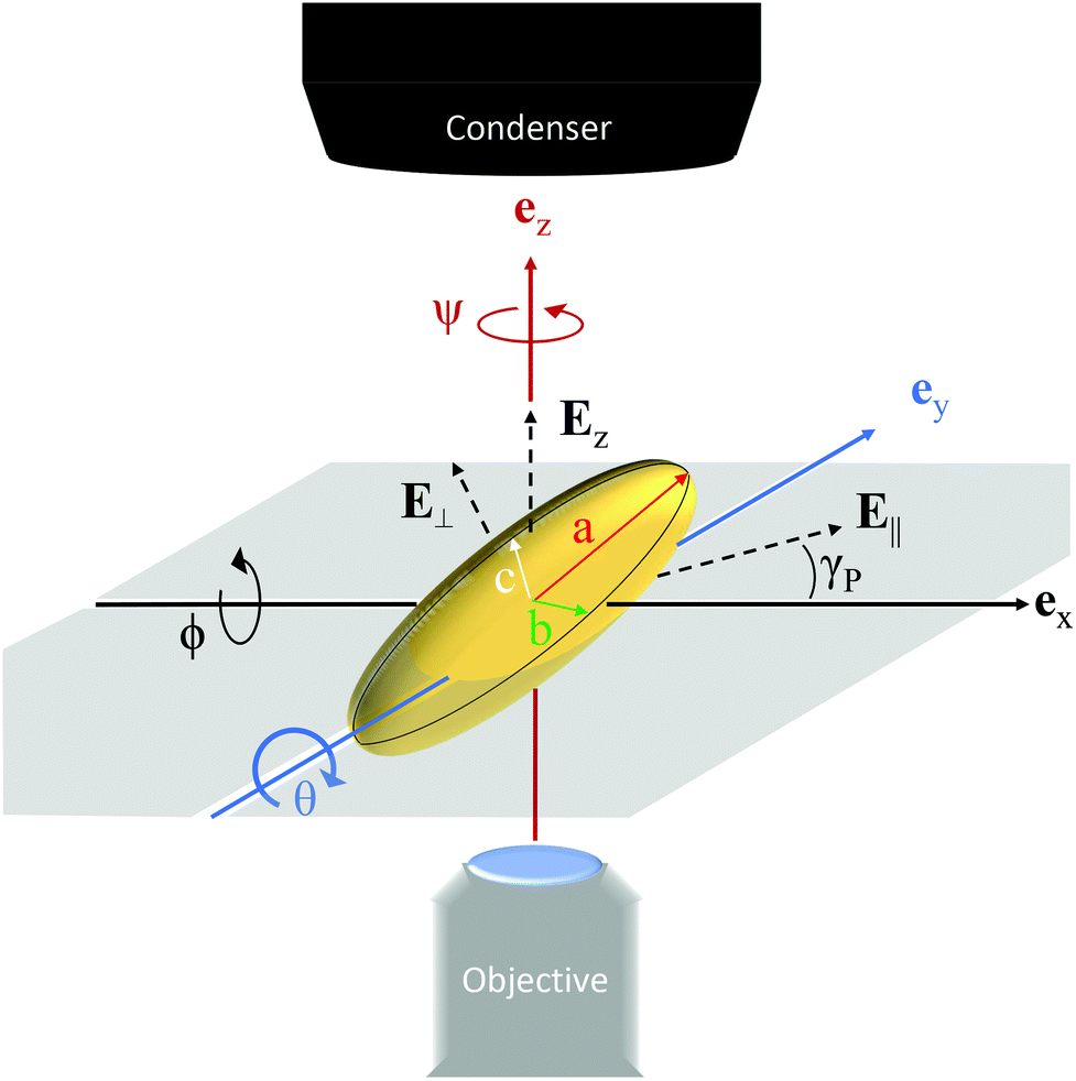 | ||
Fig. 1 A sketch of the geometry of the NP in the measurement reference system, with the +z pointing away from the objective. Note,  and and  are in the x–y plane. a, b, and c are mutually orthogonal and refer to the semi-axes of the NP, which are ordered so that a ≥ b ≥ c. Circular arrows with angles ϕ, θ, and ψ indicate the action of the rotation matrices Rϕ, Rθ, Rψ, respectively. are in the x–y plane. a, b, and c are mutually orthogonal and refer to the semi-axes of the NP, which are ordered so that a ≥ b ≥ c. Circular arrows with angles ϕ, θ, and ψ indicate the action of the rotation matrices Rϕ, Rθ, Rψ, respectively. | ||
The resulting extinction cross-section spectra are given in Fig. 2 for a gold NP of a volume given by that of a sphere of 30 nm diameter, and different aspect ratios, for fields along the NP semi-axes. Here, and in the remainder of this work, we took εNP from the tabulated values for gold from ref. 36, interpolated in 2 nm steps over the range λ = 400 nm to 800 nm. For prolate NPs, the σext for fields along the long axis (Fig. 2a top) shows the longitudinal LSPR shifting to longer wavelength and increasing in amplitude, reaching 600 nm and 105 nm2 for aspect ratios b/a around 1/2. For oblate NPs, similarly, 600 nm and 105 nm2 are reached for b/a ≈ 3 (Fig. 2b bottom). The geometrical cross-section of the sphere is about 707 nm2, which is similar to the calculated extinction cross-sections at λ = 400 nm, where gold is strongly absorptive. For NPs with three different semi-axes lengths, shown in Fig. 2c–e, the qualitative behaviour is similar, with the LSPR for a polarization along each semi-axis red-shifting with increasing axis length, but also affecting the LSPRs along the other two axes.
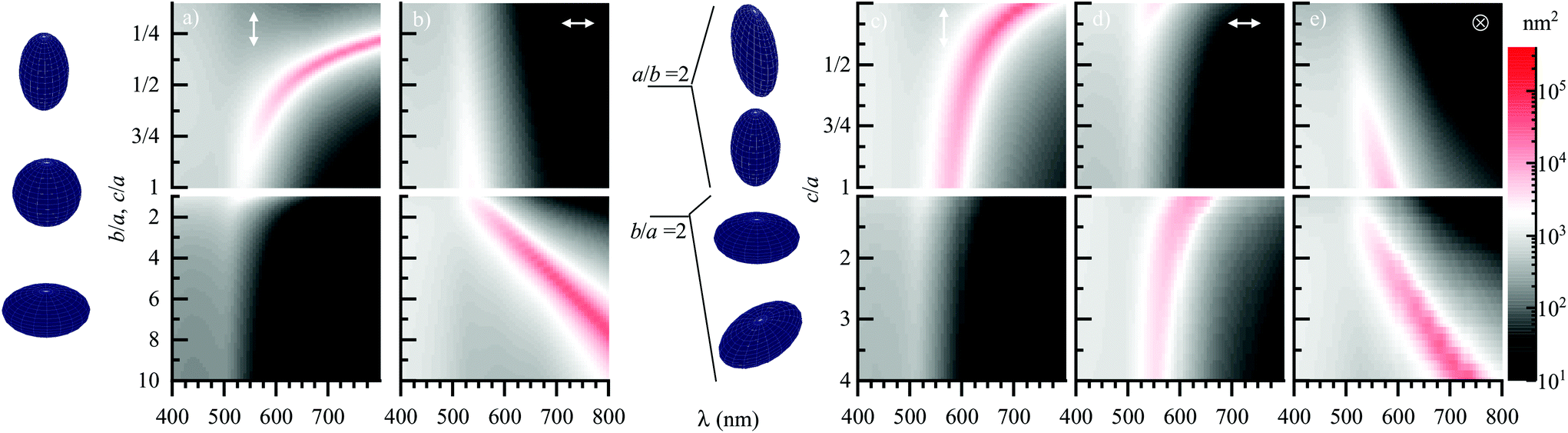 | ||
| Fig. 2 Extinction cross-section spectra σext for a GNP of constant volume equal to a D = 30 nm sphere, in n = 1.52 homogeneous environment, with varying aspect ratios. Logarithmic grey-scale from 10 to 105 nm2 as given on the right. For illustration purposes, the NP semi-axis directions are taken as vertical (a), horizontal (b), and out of drawing plane (c), and the size ordering a ≥ b ≥ c is disregarded. The incident field directions are given by the arrows, along a in (a) and (c), along b in (b) and (d), and along c in (e). GNPs in (a and b) are prolate (top) and oblate (bottom) with varying b/a = c/a, while in (c), (d), and (e) they have varying c/a for b/a = 0.5 (top), and b/a = 2 (bottom). | ||
A specific rotational formalism must be chosen in order to calculate in a consistent way. For computational reasons, we wish to remove the angle γP as an explicit parameter (as described in the ESI section S.II†), which can be achieved by having the first rotation in T given by a rotation about the z axis. We therefore define as
| = RψRθRϕ, T = RϕTRθTRψT | (11) |


so that in eqn (7), RψT is the first multiplier of

 . The rotations Rψ, Rθ, Rϕ when acting in the measurement frame are illustrated in Fig. 1. The unique angular ranges are given by ϕ ∈ [0, π], θ ∈ [−π/2, π/2], and ψ ∈ [0, π], as discussed in the ESI section S.IIA.†
We can now calculate, in the dipole limit, for a given field  , the cross-sections for an elliptical NP of orientation Ω = (ψ, θ, ϕ), described by the semi axes a ≥ b ≥ c, NP permittivity εNP, and medium permittivity εm.
The illumination in the experiment employs a polarizer at an angle γP to the x axis in the back focal plane of the condenser, and a given numerical aperture range. As a result, the field in the sample plane is a superposition of incoherent contributions of a range of incident directions and polarizations. To approximate this illumination, excitation fields  of three orthogonal directions are considered. These are the two fields in the sample plane, one along the polarizer
  , and one orthogonal
  to it, given by
 | (12) |
 | (13) |
To treat the illumination approximately, we consider an average of cross-sections for fields in the three directions  ,
,  ,
,  , with weights given by the corresponding field intensities created by the illumination (see eqn (3.16) in ref. 24). Briefly, the illumination rays are projected into the respective polarization directions, and their intensity is integrated over the illumination range. For typical illuminations, the highest intensity is along
  , followed by
  , and then
  . Specifically, for illumination with NA = 0.95 in a medium of n = 1.52, the corresponding relative field strengths are E‖ = 0.999, E⊥ = 0.044, Ez = 0.321, while for NA = 1.34, they are E‖ = 0.996, E⊥ = 0.092, Ez = 0.449, with the normalization E‖2 + E⊥2 = 1. The normalization does not consider Ez since this component is propagating orthogonal to z and is thus not contributing to the measured reference intensity. The corresponding long shadow effect is discussed in ref. 33. As a result, the illumination probes not only the response for in-plane polarization, but also to some extent the response for a polarization along the microscope axis. The expected measured absorption cross-section is then calculated as
 | (14) |
 , defining spectrally averaged absorption cross-sections
 | (15) |
The resulting extinction cross-sections for various polarizer angles γP and colour channels Λ are then compared with the corresponding measured quantities σΛ (γP), defining the normalized error
 | (16) |
![[small sigma, Greek, circumflex]](https://www.rsc.org/images/entities/i_char_e111.gif) Λ(γP) is the measurement noise of σΛ(γP). The parameter η accounts for the fact that a fraction of the scattered light is collected by the objective. In the present model, we approximate this fraction by the one for scattering by a spherical NP in a homogeneous medium, for unpolarized illumination, in the dipole limit. Using a NA of 0.95 for both illumination and collection, the fraction of scattered light collected is 13.6%,37 so that we use η = 0.864. We note that this is a small correction, and that accordingly the approximation used is appropriate. Minimising S2 over the NP parameters, we determine the most likely parameters describing the NP. We use MatLab R2018b to perform this fitting procedure, which is described in more detail in the ESI section S.II.† Typical computational times are around 1 second per NP fit on a modern CPU (AMD Ryzen Threadripper 2950X).
Λ(γP) is the measurement noise of σΛ(γP). The parameter η accounts for the fact that a fraction of the scattered light is collected by the objective. In the present model, we approximate this fraction by the one for scattering by a spherical NP in a homogeneous medium, for unpolarized illumination, in the dipole limit. Using a NA of 0.95 for both illumination and collection, the fraction of scattered light collected is 13.6%,37 so that we use η = 0.864. We note that this is a small correction, and that accordingly the approximation used is appropriate. Minimising S2 over the NP parameters, we determine the most likely parameters describing the NP. We use MatLab R2018b to perform this fitting procedure, which is described in more detail in the ESI section S.II.† Typical computational times are around 1 second per NP fit on a modern CPU (AMD Ryzen Threadripper 2950X).
3. Experiment
3.1. Optical measurements
The optical measurements reported in this work were performed on a Nikon Ti-U inverted microscope, using as illumination source either a 100 W halogen lamp with bandpass filters (center wavelengths 450 nm, 550 nm, 600 nm, 650 nm, or 750 nm) of 40 nm width, or a light emitting diode (LED) source (Thorlabs LED4D106) providing two independent LEDs of center wavelengths 530 nm and 660 nm (for their spectrum see ESI Fig. S1†) coupled via a liquid light guide (Thorlabs AD5LLG). The microscope was setup with a 1.34 numerical aperture (NA) oil-immersion condenser (Nikon MEL41410) limited to NA = 0.95 to match the 0.95NA 40× dry objective (Nikon MRD00405) used with the 1.5× tube-lens. The image data was recorded using a scientific-CMOS (sCMOS) camera (PCO Edge 5.5), capable of acquiring 100 frames per second (FPS) at 2560 × 2160 pixels with 16 bit digitization, 0.54 electrons per count, and a full well capacity of Nfw = 30![[thin space (1/6-em)]](https://www.rsc.org/images/entities/char_2009.gif) 000 electrons. The illumination intensity and exposure time was chosen to be close to Nfw without entering the range of non-linear response. A sketch of the setup is given in Fig. 3.
000 electrons. The illumination intensity and exposure time was chosen to be close to Nfw without entering the range of non-linear response. A sketch of the setup is given in Fig. 3.
 | ||
| Fig. 3 Sketch of the imaging setup used. The transmission of a sample under Köhler illumination of a defined linear polarization and selectable wavelength range is imaged onto a sCMOS camera, using a condenser and an objective of matched high numerical apertures. The sample position is laterally shifted by a piezoelectric stage for referencing. | ||
3.2. Structural characterization
Transmission electron microscopy (TEM) was performed on a JEOL-JEM 2100 TEM operating at 200 kV, with samples prepared on 300 Mesh holey carbon. High-angle annular dark-field scanning transmission electron microscope (HAADF-STEM) images and tomography series were acquired using a FEI Osiris microscope operated at 200 kV. The tomography series were acquired over the tilt range of ±75° with a tilt increment of 3° using a Fischione 2020 single-tilt tomography holder and a pixel dwell time of 6 μs. After alignment of the projection images by using a cross correlation, the stacks of aligned projection images served as inputs for 20 iterations of the expectation maximization reconstruction algorithm implemented in the ASTRA toolbox 1.9.0 using Matlab 2019a.38,39 Amira 5.4.0 was used for the 3D visualization.3.3. Samples and their preparation for optical measurements
GNPs of nominal spherical shape and mean diameters of 20 nm (GNSs) were obtained from BBI Solutions. Branded ‘ultra-uniform GNPs’ of nominal spherical shape and mean diameter of 30 nm (UGNSs) were obtained from NanoComposix. Finally, gold nanorods (GNRs) of nominal dimensions (30 × 10 × 10) nm3 were obtained from NanoPartz. Glass slides and coverslips (Menzel-Gläser, #1.5) were cleaned by sequential sonication phases in toluene to remove non-polar substances, acetone to clear the toluene, and then rinsed and boiled in deionised (DI) water. Slides and coverslips were then left in 30% hydrogen peroxide until needed, allowing oxidation of remaining surface contaminants, as well as hydrophilising the glass surfaces. Prior to NP deposition, any required glass was washed with DI water. The NP colloid was diluted with water to a final concentration of 108 NP per ml, and a volume of 200 μl was spin-coated onto the coverslips at 2000 RPM for 2 minutes, with an acceleration time of 30 seconds. This procedure provided an areal density of NPs of (0.1–0.4) NP per μm2, such that most NPs visible in the image are resolved individuals with well-separated point spread functions (PSF). The NP side of the coverslip was coated in 18 μl of refractive index n = 1.52 silicone oil, and covered with a slide. The samples were then sandwiched between two pieces of cleanroom grade optical paper and two more glass slides. The unsealed construction was then slowly pressed in a table vice and the oil allowed to leave for a few minutes soaking into the optical paper. This process was continued until the outer glass slides exhibited a subtle, but audible, crack. The outer slides and paper were removed, and the original coverslip and slide were then sealed with clear nail varnish. This process resulted in an oil layer below 1 μm thickness, so that the slide surface and the NPs on the coverslip surface were close to focus at the same time. As a result, debris on the slide surface creates a spatially localized perturbation, affecting only a small fraction of the total sample area.3.4. Measurement of extinction
We use a method to quantitatively measure σext, which has been described in ref. 31, 32 and 37. Briefly, two offset-subtracted brightfield images are obtained; the signal, I1, with NPs in focus at position, P1 = (x1, y1), and the reference, I2, with the sample laterally shifted to position, P2 = (x2, y2) = (x1 + δx, y1 + δy), with the magnitude of the shift, . Generally, I1 and I2 are averaged over a number, Ni, of individual acquisitions, reducing shot noise in the final image. The normalised transmission is obtained by
 | (17) |
 | (18) |
 | ||
| Fig. 4 Examples of Δ+ (right, triple colour channel overlay) and σΛ (γP) (left) for different polarizer angles γP and three colour channels Λ, along with fits using eqn (21). (a) GNR, colour channel range in Δ+ is ±0.76%. Imaging parameters were Ni = 128, Nr = 10, such that ext = (49.7, 51.5, 92.5) nm2 for Λ = (550, 650, 750). (b) UGNS, colour channel range in Δ+ is ±0.8%. Imaging parameters were Ni = 128, Nr = (4, 4, 16), such that ext = (57.5, 53.1, 30.9)nm2 for Λ = (450, 550, 600). The total acquisition time for the 18 Δ images covering all polariser angles and wavelengths was about 4 min. The full acquired field of Δ+ is given in the ESI Fig. S2.† | ||
3.5. Analysis of σext
To measure the cross-section of a NP at P1 in Δ+, we integrate Δ+ over an area, Ai, of radius, ri, centred at P1, and Δ− over the corresponding area at P2, such that the extinction cross-section is given by | (19) |
The shot-noise limited noise in the measurement of σext is given by32
 | (20) |
ext of about 50 nm2, and are shot-noise limited with increasing Na down to about 4 nm2. Below this value, surface roughness, debris, residual sensor fluctuations etc. are affecting the results for our setup and samples. To achieve ext < 1 nm2, we can employ additional procedures as described in ref. 32, which were not used in the present work.
When measuring σext as a function of the excitation polarizer angle γp, we fit the data with
| σ(γp) = σ[1 + αcos{2(γp − γ)}], | (21) |
Examples of this analysis are given in Fig. 4, where Fig. 4a shows results for a NP with strong asymmetry, from the GNRs. For Λ = (550, 650, 750), this NP is described by αΛ = (0.042, 0.84, 0.94), σΛ = (290, 427, 1087) nm2, and γΛ = (138.9, 1.1, 177.8)°, hence we can infer an orientation of the long axis of the NP with γ ≈ 0 considering both Λ = 650 and Λ = 750 which are considerably red-shifted with respect to the resonance of a spherical GNP in the dipole limit. Conversely, the NP is nearly invisible for γP ≈ 90°. Additionally, we can see a significant polarisation-dependence for Λ = 650 and Λ = 750, but not for Λ = 550. This is consistent with the redshift of the LSPR polarized along the long axis.
Fig. 4b instead shows a NP with low asymmetry, from the UGNSs. For Λ = (550, 650, 750), this NP is described by αΛ = (0.067, 0.043, 0.048), σΛ = (614, 1172, 217) nm2, and γΛ = (75.5, 64.4, 79.1)°. A weak polarisation dependence is observed for all three Λ, and the NP is visible in Δ+ at both polariser angles shown. It exhibits the largest cross-section for Λ = 550, consistent with the expected wavelength dependence discussed in section 2.
4. Results and discussion
Here we discuss the results of the analysis of σext for hundreds of individual NPs of different types. Particular care needs to be taken in understanding the meaning of the statistical distribution of the cross-sections across a set of NPs. Information related to the size and shape distributions is contained within the NP set. Yet, each measured quantity on an individual NP will be affected by the error due to the measurement noise. The evaluation of these effects is discussed below.4.1. Distributions of σΛ and αΛ
The distribution of αΛversus σΛ is shown in Fig. 5 for three sets of NPs, together with batch-representative TEM images. We call the mean of the polarisation-averaged cross-sections for a given colour channel![[small sigma, Greek, macron]](https://www.rsc.org/images/entities/i_char_e0d2.gif) Λ, and the associated standard deviation Λ,m. We call the analogous properties of the α parameter
Λ, and the associated standard deviation Λ,m. We call the analogous properties of the α parameter ![[small alpha, Greek, macron]](https://www.rsc.org/images/entities/i_char_e0c2.gif) Λ and Λ,m. For each NP, we determine the error of the fitted parameters σ, α, and γ, using a Monte Carlo-like simulation. In detail, we add random noise to the measured data, from a Gaussian distribution with a root mean square (RMS) given by the experimentally determined noise ext for each γP and Λ, refit the data, and use the RMS of the resulting parameter distribution as error. Let us in particular denote the standard deviation of the per-NP fitted parameter σi by Λ,i, where i numbers the N NPs. To remove the measurement noise from Λ,m, we define
Λ and Λ,m. For each NP, we determine the error of the fitted parameters σ, α, and γ, using a Monte Carlo-like simulation. In detail, we add random noise to the measured data, from a Gaussian distribution with a root mean square (RMS) given by the experimentally determined noise ext for each γP and Λ, refit the data, and use the RMS of the resulting parameter distribution as error. Let us in particular denote the standard deviation of the per-NP fitted parameter σi by Λ,i, where i numbers the N NPs. To remove the measurement noise from Λ,m, we define  , which represents only the distribution of NP cross-sections across the various NPs, due to their different sizes and shapes. Note that for Λ, m this correction has not been done, since the corresponding standard deviations Λ,i vary strongly depending on Λ,m and Λ, and we use Λ = Λ,m.
 | ||
Fig. 5 Asymmetry αΛversus cross-section σΛ for sets of different NPs and channels Λ as given, with representative TEM images of the investigated NP batch on the right. Left inset: σΛvs. σΛ′ as labelled. Right inset: αΛvs. αΛ′ as labelled. Both on a range as indicated. In all cases, Ni = 128. (a) 223 UGNSs using Nr = (4, 4, 16) for Λ as labelled, yielding ext = (57.5, 53.1, 30.9) nm2. (b) 129 GNSs using Nr = 4 for both Λ as labelled, yielding ext = (44.1, 45.8) nm2. (c) 95 GNRs, using Nr = 10 for all Λ as labelled, yielding ext = (49.7, 51.5, 92.5) nm2. The error bars are showing the error of σΛ of the respective colour channels, given by  . The grey areas indicate the noise in the fitted α of the red channels due to ext, estimated as . The grey areas indicate the noise in the fitted α of the red channels due to ext, estimated as  . . | ||
600 ± 600 = 0.058 ± 0.031, indicating NPs of very low ellipticity. 450/450 and 550/550 are both about 18%. At these wavelengths the cross-section is roughly proportional to the NP volume, hence 18% relative volume distribution corresponds to 6% radius distribution. 600/600 instead is larger, about 41%, consistent with the fact that the variability of σext at a wavelength above the LSPR of a spherical NP is sensitive to shape deviations, in fact elliptical shapes result in a red-shifted σext as shown in Fig. 2. This can also be seen in the correlation of increasing σ600 with α600 for the outliers having larger deviations from the spherical shape in Fig. 5a. Notably, correlating σ600 with σ550 (see inset), two groups can be identified, with different ratios σ600/σ550, identifying two distinct shapes. Qualitatively, these observations are consistent with TEM, where most of these ultra-uniform NPs are defect-free and have a faceted shape, while a few NPs contain defects and hence vary from these shapes, as shown in the ESI section S.III.† Additionally, we see that 550 > 450 > 600 as expected for spherical gold NPs with a LSPR at λ ≈ 530 nm in a homogeneous environment of nr = 1.52.
Fig. 5b shows the results for a set of GNSs, which we measured using LED illuminations centred at 530 nm and 660 nm. For this sample, the TEM indicates a large variability in shape, dominated by multicrystalline roundish NPs, and monocrystalline triangular plates with rounded edges. The plates are seen also side-on, where they appear rod-shaped. Indeed, we find that the measured σΛ is highly distributed for both available Λ, with 530 ± 530 = (645 ± 469) nm2, and 660 ± 660 = (298 ± 482) nm2. For many NPs in this sample, σ660 is comparable to the noise level, with ext = 43 nm2, resulting in a large error of α660, as estimated by the dashed line. Nonetheless, for NP with larger σ660, also a large α660 is observed, consistent with the presence of plate-like shapes in TEM. Likewise, α530 ranges from about 0 to 0.4, with most values below 0.25 (530 ± 530 = 0.12 ± 0.18), indicating that on average the NPs have some distinct non-sphericity. The large value of 530/530 ≈ 57% suggests a wide distribution in average size as well. However, 530 > 660, showing that most NPs do not have an aspect ratio above 1.5 (see Fig. 2), consistent with TEM analysis (see also Table 1 and ESI Table S1†).
| NP type |
![[p with combining macron]](https://www.rsc.org/images/entities/i_char_0070_0304.gif) D
v
±
D
v
± ![[p with combining circumflex]](https://www.rsc.org/images/entities/i_char_0070_0302.gif) Dv (nm) Dv (nm) |
b/a ± b/a |
|---|---|---|
| 30 nm UGNS | 28.59 ± 1.77 | 0.973 ± 0.024 |
| 20 nm GNS | 17.84 ± 1.25 | 0.865 ± 0.091 |
| 30 × 10 × 10 nm3 GNR | 15.36 ± 2.86 | 0.394 ± 0.135 |
650 > 550, and a ratio 650/750 around one, increasing with aspect ratio. We find that 650 = 867 nm2 and 750 = 935 nm2 are indeed larger than 550 = 580 nm2. The variabilities of σΛ and αΛ are large, with Λ/Λ > 83% and Λ,m/Λ > 43% for all Λ, indicating a significant distribution of both shapes and sizes. Additionally, 550 = 0.2, 650 = 0.62, and 750 = 0.72 indicate that the NPs have a large optical asymmetry. This is consistent with the TEM for this batch, which shows nanorods in the size range indicated by the manufacturer (nominal (30 × 10 × 10) nm3) alongside quasi-spherical NPs smaller than 10 nm, rods with aspect ratios as large as 10:1, and some other shapes.
4.2. NP geometry determined by fits
The primary goal of this work is to determine NP size and shape by comparing the data with a parameterized model, and determine the most likely parameters by minimizing the weighted error between model and experimental data, as given in eqn (16). We implemented this minimization in MatLab R2018b. To best use the optimized vector/matrix operations of Matlab, portions of the various equations described in section 2, such as constants defined as integrals over spectral ranges, were brought outside the parameterized parts of calculations. A gridded multi-dimensional parameter space was created, allowing for two rotation angles (note that the angle ψ is contained in the polarizer angle γP), and two shape parameters via semi-axes aspect ratios b/a ∈ [ι1, ι2] and c/a ∈ [ι1, ι2]. We used ι1 = 0.25 to ι2 = 1.43 for the UGNSs, and ι1 = 0.1 to ι2 = 1.75 for the GNSs and GNRs to cover the broader spread in shapes. We then calculated σabs(γP,Λ)/V and σsca(γP,Λ)/V2 at each grid point, and obtained an interpolant of their values between the grid points using an Akima piecewise cubic function. The experimental data were compared to all calculated values on the grid viaeqn (16). The right side of eqn (16) is a fourth order polynomial in the volume, V. We therefore minimized S2versus V using the analytical roots of the third-order polynomial equation , yielding S and V for all points on the grid. The points which are local minima of S on the grid, and have an error below a threshold, S < σc, were then used as initial guesses for a gradient descent minimizing S2 using the interpolation. Initial guesses with equal error within the numerical precision were considered to be rotational redundancies, and only one of each of these degenerate cases was used to reduce computational effort. The resulting set of errors and parameters obtained over all gradient descents is called the minimized set. Assuming we have no further information at hand, the element of the minimized set exhibiting the minimum error S is the most likely to describe the size, shape, and orientation of the NP.
Firstly, we checked the validity of this fitting procedure using synthetic data of gold NPs with given size and shape, and verified that the fit was converging to the expected values. Then, we examined the distribution of fitted parameters when adding the experimental noise to synthetic data. An example of this analysis is shown for prolate gold NPs in Fig. 6. The data are calculated matching the experimental conditions, including Λ and γP, of the UGNSs in Fig. 5a. The cross-section data to be fitted were calculated for a NP of a volume characterized by the sphere-equivalent diameter DV = 25.6 nm (taken from the average of the fitted  in Fig. 7), and of an orientation ψ = θ = ϕ = 0, so that a and b are in the measurement x, y plane. The distribution of fitted parameters results from the set of noise realizations, with ext = (57.5, 53.1, 30.9) nm2 for Λ = (450, 550, 600), respectively. These values of ext correspond to the measurements in Fig. 5a, and amount to 2–20% of the respective σext. The different colors in the plots show different simulated aspect ratios b/a = c/a as indicated. The fit parameter space is 6-dimensional (three orientation angles and three semi-axis lengths), and we have 18 simulated measurements (6 γP at 3 Λ). Notably, measuring a spherical NP (b/a = c/a = 1), the noise results in fitted values of aspect ratios between 1 and 0.8. For a strongly prolate NP instead (e.g. b/a = c/a = 0.6), the average aspect ratio
  is rather well defined (see right inset, e.g. magenta histogram), while b/a and c/a still vary significantly. The retrieved volume (see histogram in left inset) shows a smaller dependence on the aspect ratio, while still being of decreasing variation with decreasing aspect ratio. Reducing the measurement noise, the distributions narrow, as shown in the ESI Fig. S3.† Equivalent simulations for the oblate and general cases are discussed in the ESI section S.IIC.† Generally, the interplay between NP orientation, aspect ratios, and probed colour channels goes beyond an intuitive understanding for all but the simplest cases. Nevertheless, we see that a suited choice of colour channels and measurement noise allows retrieval of NP shapes and sizes. Notably, the colour channel choice can be informed by this type of simulation, by evaluating the errors of fitted sizes and shapes for a given measurement noise for different combinations of available colour channels.
 | ||
Fig. 6 . Evaluation of fit results for synthetic data. Fitted c/a and b/a using 1000 measurement noise realizations for a prolate gold NP with constant volume equivalent to a sphere of diameter, DV = 25.6 nm, for various b/a = c/a as indicated(see also circle symbols), and ψ = θ = ϕ = 0. The polarization averaging (eqn (14)) was done for an illumination NA of 0.95. A noise of ext = (57.5, 53.1, 30.9) nm2, was used for the color channels Λ = (450, 550, 650), respectively, taken from the UGNS experiment in Fig. 5a. Top inset: Extinction spectra at γP = 0, for b/a = 1 (black), b/a = 0.6 (magenta). The bands indicate the spectral ranges Λ used. Right inset: Histograms of fitted  for b/a as colour coded. Left inset: Histogram of the fitted volume V for b/a as colour coded. for b/a as colour coded. Left inset: Histogram of the fitted volume V for b/a as colour coded. | ||
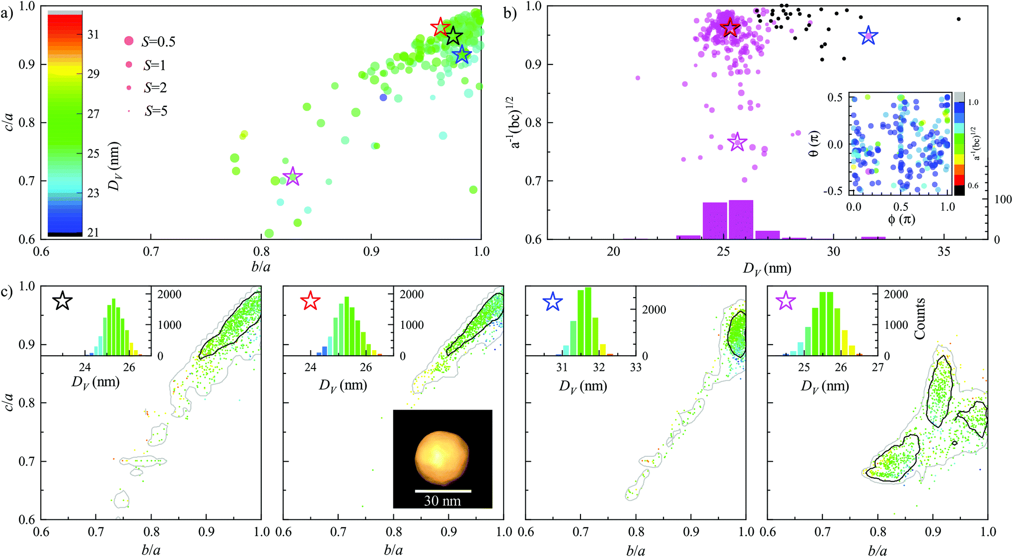 | ||
Fig. 7 Fitted parameters for UGNSs using the channels Λ = 450, 550 from the measurements shown in Fig. 5a. (a) c/a versus b/a, with the colour scale indicating the volume equivalent diameter DV. (b) magenta points: geometric average aspect ratio,  , versus DV. Black points: b/a versus , versus DV. Black points: b/a versus , for 30 NPs examined using TEM. The magenta bars give the histogram of the magenta points. In both (a) and (b), the size of the points is given by S− = 1/(1 + S), so larger points indicated lower error, as shown in (a). Inset in (b) shows the fitted NP orientation angles θ versus ϕ, with the colour indicating , for 30 NPs examined using TEM. The magenta bars give the histogram of the magenta points. In both (a) and (b), the size of the points is given by S− = 1/(1 + S), so larger points indicated lower error, as shown in (a). Inset in (b) shows the fitted NP orientation angles θ versus ϕ, with the colour indicating  . (c) For the measured NPs indicated by stars in (a and b), fit results for 10000 realizations (1000 shown by filled circles) of added random measurement noise. Contours are the boundaries of regions of highest density containing 68% (black) and 95% (grey) of the data. Insets show the distributions of DV, and provide the symbol colour scale. The inset in the red starred plot is a TEM tomographic reconstruction of an exemplary NP (see also ESI section S.III†) from the same sample stock with similar DV as the fitted NP. . (c) For the measured NPs indicated by stars in (a and b), fit results for 10000 realizations (1000 shown by filled circles) of added random measurement noise. Contours are the boundaries of regions of highest density containing 68% (black) and 95% (grey) of the data. Insets show the distributions of DV, and provide the symbol colour scale. The inset in the red starred plot is a TEM tomographic reconstruction of an exemplary NP (see also ESI section S.III†) from the same sample stock with similar DV as the fitted NP. | ||
Prior knowledge, such as ensemble size specifications from the NP manufacturer, can also be taken into account to determine the most likely NP geometry. We perform such a selection as a post-fit routine, comparing the fitted parameters in the minimized set with those of prior knowledge for each NP. We then select the parameter set exhibiting the minimum “combined error” after this comparison. Using the mean i and variance i for the parameters i ∈ {DV, b/a, c/a} taken from TEM, we add an error related to the deviation from expected values to arrive at the combined error Sc given by
 | (22) |
The values of i and i used for the different NP types are given in Table 1. Since TEM is measuring only two sizes, we set b/a = c/a and b/a = c/a.
 , and the symbol size indicating the fit error S. We find that c/a and b/a are mostly above 0.9, and the DV ranges between 24 and 27 nm. Fig. 7b shows the average aspect ratio
  versus DV, and a histogram of DV. Notably, the values of DV are about 10% smaller than measured in TEM, the latter shown as black points in Fig. 7b (see also ESI Fig. S14† for a comparison with 2D projection HAADF-STEM). A possible explanation of this small discrepancy is the fact that in TEM we measure only the NP size in plane, and the corresponding values in Fig. 7b are calculated using
  .
.
To appraise the measured parameter distributions, it is again important to understand the effect of the measurement noise characterized by ext. To this end, four measured NPs were selected, indicated by (black, red, blue, magenta) stars in Fig. 7a, which have α550 = (0.092, 0.026, 0.023, 0.203), and σ550 = (1150, 1117, 2566, 1473) nm2, respectively. Random Gaussian noise of standard deviation ext was added to the experimental data, and the NP parameters were retrieved from the resulting data. This was repeated for 10000 noise realizations, and the results are shown in Fig. 7c, each NP in a separate panel. The contours indicate the regions of highest probability density containing 68% and 95% of the data, which for a Gaussian distribution are the σ and 2σ confidence intervals, respectively. The results show that, depending on the NP size and shape, the measurement noise results in about 1 nm full-width-at-half maximum (FWHM) in DV, and 10% in b/a and c/a. These values account for about half the parameter spread in the set of investigated UGNSs, confirming that the size and shape distribution of these NPs is indeed very uniform.
The NPs indicated by the black and red stars show a confinement of the data to b ≈ c, which is consistent with the simulated result in Fig. 6 for a spherical NP. The blue star NP shows a tighter distribution due to its high cross-section, reducing the effect of noise. The measured in-plane anisotropy is very small (2.3%) for this NP, and the fit shows a slightly oblate particle with b/a > 0.95, c/a ≈ 0.92, and the c semi-axis along z in the measurement system, as in Fig. S4.† The magenta star NP has a sizeable anisotropy (20.3%) and three different semi-axes, with c/a ≈ 0.71 and b/a ≈ 0.82. Overall, we see that the measurements give detailed information about these nominally 30 nm diameter NPs, with diameter precision around 1 nm and anisotropy precision in the 10% range for a measurement noise around 50 nm2. Decreasing the measurement noise by about an order of magnitude would increase the precision, as seen in Fig. S3,† and is possible with the experimental technique.32 Notably, the precision of the diameter would increase by the same factor, while for the asymmetry, the situation is more complex. For an isotropic case, the degeneracy of all semi-axes allows for a larger parameter space resulting in similar cross-sections, while for a significantly asymmetric NP, this degeneracy is at least partially lifted, reducing the resulting parameter uncertainty. This is exemplified in the simulated cases seen in Fig. S4 and S5† comparing c/a = 1.0 with c/a = 0.6, and for three distinct semi-axes in the ESI Fig. S6.†
The fitted angles are shown in the inset of Fig. 7b. In particular we plot θ and ϕ, the two angles which rotate the NP out of the substrate plane. The in-plane rotation ψ creates only a shift in the measured dependence of σΛ(γP) on γP, and thus does not change the measured cross-section set. The observed angular distribution is spread over the full ranges of ϕ and θ, consistent with the near spherical shape of the NPs. Some reduction around |θ − π/2| = 0, and around |ϕ| = π/2 is visible, which we can understand considering that as soon as there is some asymmetry, the NP is more likely to lie down on the substrate plane, so that a and b are in the substrate plane, corresponding to θ = ϕ = 0, as opposed to standing on end, which is either θ ≈ π/2 (a normal to substrate), or θ ≈ 0 and |ϕ| ≈ π/2 (b normal to substrate).
To determine the full three-dimensional NP shape with EM, going beyond 2D projection TEM as shown in Fig. 5, we have performed high-angle annular dark-field scanning transmission electron microscope (HAADF-STEM) tomography for a few of the UGNSs, as described in the ESI section S.III.† We found that most NPs are mono-crystalline and nearly spherical, consistent with our optical measurements and discussed fitting results. The aspect ratios of two NPs obtained from tomography are 0.99 and 0.96. For illustration one 3D rendering is shown in the inset of Fig. 7c.
We note that the selection of color channels Λ influences the results to some extent, as different channels are sensitive to different NP parameters and shape ranges, as discussed in detail in the ESI section S.II E.† Using {Λ} = {450, 600} is found to produce oblate NPs in the fit, which shows that the model underestimates the cross-section in the Λ = 600 channel. This can be attributed to the neglected surface damping20,25 in the gold permittivity used in our model, and the absence of surface faceting in the ellipsoidal shape assumed.
We now move to the more conventional GNSs, which, as we have seen in Fig. 5b, have a more variable shape. This is visible also in the fit results shown in Fig. 8, where there are rod-shaped NPs with b/a ≈ c/a < 0.6, plates with b/a > 0.8 and c/a < 0.5, and reasonably spherical NPs with c/a > 0.7, as indicated in Fig. 8a. The distribution of the diameter results in a mean ![[D with combining macron]](https://www.rsc.org/images/entities/i_char_0044_0304.gif) = 21.8 ± 5.8 nm. We see a narrow mode around 18 nm, in good agreement with the observations from TEM (black dots in Fig. 8b). The comparison with results of 2D projection HAADF-STEM are given in the ESI Fig. S13.† A tail of outliers to higher volume with a small aspect ratio is also found. Such NPs are not obvious in the TEM data, which mainly show roundish NPs with defects, and triangular plates in either side or top view. They could be thin plates of larger size, which are sporadically seen in TEM, and possibly NP dimers formed by aggregation. We also note that by dropping the Λ = 450 channel compared to the UGNS data shown in Fig. 7, the NP volume is less constrained. The orientation of the NPs (inset in Fig. 8b) shows again a broad distribution, but with a stronger tendency to lie flat (θ ≈ 0, | ϕ − π/2| ≈ π/2), consistent with the larger deviation from spherical shape. To assess the effect of the measurement error, also in this case four measured NPs were selected, indicated by (black, red, blue, magenta) stars. Random Gaussian noise of standard deviation ext was added to the experimental data, and the NP parameters were retrieved. The corresponding distributions are shown in Fig. 8c. We find an uncertainty in the diameter of about 2 nm FWHM in DV and 20% in b/a and c/a, larger than in the case of Fig. 7c, because the NPs, and therefore the cross-sections, are smaller, resulting in a lower signal to noise ratio. Nonetheless, the method clearly separates different NPs, and highlights the fairly broad distribution of NP sizes and shapes in this sample. Also here, we have performed tomographic TEM for a few of the GNSs, as described in the ESI section III.† We found, consistent with the above fitting results, that the NPs look rather irregular, with some pentatwinned NPs but also many other spherical-like irregular shapes. Almost all NPs contain lattice defects. Note that lattice defects provide additional scattering sites for the free electrons of the metal, affecting εNP, as discussed in the ESI sec. II.D.† The aspect ratios obtained from tomography for two GNSs are 0.9 and 0.813. For illustration, one 3D rendering is shown in the inset of Fig. 8c.
= 21.8 ± 5.8 nm. We see a narrow mode around 18 nm, in good agreement with the observations from TEM (black dots in Fig. 8b). The comparison with results of 2D projection HAADF-STEM are given in the ESI Fig. S13.† A tail of outliers to higher volume with a small aspect ratio is also found. Such NPs are not obvious in the TEM data, which mainly show roundish NPs with defects, and triangular plates in either side or top view. They could be thin plates of larger size, which are sporadically seen in TEM, and possibly NP dimers formed by aggregation. We also note that by dropping the Λ = 450 channel compared to the UGNS data shown in Fig. 7, the NP volume is less constrained. The orientation of the NPs (inset in Fig. 8b) shows again a broad distribution, but with a stronger tendency to lie flat (θ ≈ 0, | ϕ − π/2| ≈ π/2), consistent with the larger deviation from spherical shape. To assess the effect of the measurement error, also in this case four measured NPs were selected, indicated by (black, red, blue, magenta) stars. Random Gaussian noise of standard deviation ext was added to the experimental data, and the NP parameters were retrieved. The corresponding distributions are shown in Fig. 8c. We find an uncertainty in the diameter of about 2 nm FWHM in DV and 20% in b/a and c/a, larger than in the case of Fig. 7c, because the NPs, and therefore the cross-sections, are smaller, resulting in a lower signal to noise ratio. Nonetheless, the method clearly separates different NPs, and highlights the fairly broad distribution of NP sizes and shapes in this sample. Also here, we have performed tomographic TEM for a few of the GNSs, as described in the ESI section III.† We found, consistent with the above fitting results, that the NPs look rather irregular, with some pentatwinned NPs but also many other spherical-like irregular shapes. Almost all NPs contain lattice defects. Note that lattice defects provide additional scattering sites for the free electrons of the metal, affecting εNP, as discussed in the ESI sec. II.D.† The aspect ratios obtained from tomography for two GNSs are 0.9 and 0.813. For illustration, one 3D rendering is shown in the inset of Fig. 8c.
 | ||
| Fig. 8 As Fig. 7, but for GNSs, and Λ = 530, 660. | ||
 . The volume has been calculated assuming a cylindrical shape. These findings are in line with observations from TEM, and the optical results in Fig. 5d. We do see a large proportion of cases with b/a and c/a around 1/3, as expected from the nominal specifications, and TEM (see also ESI Fig. S14† for a comparison with 2D projection HAADF-STEM). Importantly, the individual NP fits shown in the lower four panels exhibit narrow bands at small values of c/a and b/a, similarly to the synthetic cases seen in Fig. 6. The NP orientations (see inset Fig. 9b) are distributed in ϕ but concentrated around θ = 0, as expected for rods, where ϕ is rotating around the rod axis, having little effect, and θ is tilting the rod axis out of plane. Additionally, a fraction of NPs, such as the black star one, are plate-like, with c/a < 0.25 and b/a > 0.5. Again we have performed tomographic TEM for a few of the GNRs, as described in the ESI section S.III.† We found, consistent with the above fitting results, that almost all NPs are defect free, and rod-shaped NPs are dominating. The aspect ratios obtained from tomography for two NPs are 0.36 and 0.42. For illustration, one 3D rendering is shown in the inset of Fig. 9c.
 | ||
Fig. 9 As Fig. 7, but for the GNRs and Λ = 550, 650, 750. Considering a cylindrical shape, the equivalent diameter (black points) was determined as  . . | ||
5. Conclusions and outlook
To summarise, we have demonstrated a rapid, quantitative and accurate method to “optically size” hundreds of individual nanoparticles, by measuring their optical cross-sections in widefield extinction microscopy for different light wavelengths and excitation polarizations, and solving the inverse problem of determining the particle size, shape and orientation from the measurements.We have shown examples for three different gold nanoparticle samples, nominally spherical and rod-like, in practice exhibiting various sizes and shapes, which were fitted using an ellipsoid model in the dipole limit. The results are, in general, in good agreement with non-correlative 2D projection TEM and HAADF-STEM, and HAADF-STEM tomography of the same batches. Depending on the experimental noise and the choice of colour channels in the measurements, we have quantified the sensitivity of the method. We show an uncertainty down to about 1 nm in mean diameter, and 10% in aspect ratios when using two or three colour channels and an experimental noise of about ext = 50 nm2. Notably, the precision can be increased by decreasing the measurement noise.
As an outlook, further advances in the method on the experimental side could include the direct probing of the nanoparticle axial direction, through the addition of a radial polarizer and a high numerical aperture illumination lens to generate an axial polarization component. This would improve the capability of the technique to measure particle geometries in 3D, presently originating from the interplay between particle shapes and plasmon resonance shifts. On the modelling side, calculating the response using a fully numerical solver, e.g. via COMSOL as presented in ref. 25 and 40, and optimizing the material permittivity used, would enable a more accurate and general description of essentially arbitrary shapes and material types. Combined, these future developments are poised to provide a powerful nanoparticle sizing method by optical means, presenting an alternative to complex and expensive TEM tomography analysis, merging accuracy with simplicity of use, easy access to statistics over large particle sets, and applicability to any nanoparticle size, shape, and composition.
Author contributions
L.P., W.L. and P.B. conceived the work. L.P. prepared the samples for the optical measurements and performed the related measurements and data analysis. W.A. prepared the samples for the STEM tomography, and performed the related measurements and data analysis. L.P, P.B. and W.L. developed the numerical model and fitting methods. L.P. performed the numerical simulations and data fitting. All authors contributed to the data interpretation and writing of the manuscript.Data availability
Information on the data underpinning the results presented here, including how to access them, can be found in the Cardiff University data catalogue at http://doi.org/10.17035/d.2020.0107215015.Conflicts of interest
There are no conflicts to declare.Acknowledgements
This work was supported by a Welsh Government Life Sciences Bridging Fund (grant LSBF/R6-005) and by the UK EPSRC (grant no. EP/I005072/1 and EP/M028313/1). PB acknowledges the Royal Society for her Wolfson research merit award (grant WM140077). The authors acknowledge funding from the European Commission (Grant EUSMI E191000350). WA acknowledges an Individual Fellowship from the Marie Sklodowska-Curie actions (MSCA) under the EU's Horizon 2020 program (Grant 797153, SOPMEN), and Sara Bals for supporting the STEM measurements. The bright-field TEM was performed by Thomas Davies at Cardiff University. We acknowledge Attilio Zilli for helpful discussions and contributions in calculating the relative field strengths in the illumination and finite-element simulation of cross-sections shown in the ESI.† We acknowledge Iestyn Pope for technical support of the optical equipment.References
- T. Sun, Y. S. Zhang, B. Pang, D. C. Hyun, M. Yang and Y. Xia, Angew. Chem., Int. Ed., 2014, 53, 12320–12364 CAS.
- X. Han, K. Xu, O. Taratulab and K. Farsadc, Nanoscale, 2019, 11, 799–819 RSC.
- J. Kneipp, ACS Nano, 2017, 11, 1136–1141 CrossRef CAS PubMed.
- R. M. Pallares, N. T. K. Thanh and X. Su, Nanoscale, 2019, 11, 22152–22171 RSC.
- L. Liu and A. Corma, Chem. Rev., 2018, 118, 4981–5079 CrossRef CAS PubMed.
- H. Atwater and A. Polman, Nat. Mater., 2010, 9, 205–213 CrossRef CAS PubMed.
- W. D. Pyrz and D. J. Buttrey, Langmuir, 2008, 24, 11350–11360 CrossRef CAS PubMed.
- R. Vogel, G. Wilmott, D. Kozak, G. S. Roberts, W. Anderson, L. Groenewegen, B. Glossop, A. Barnett, A. Turner and M. Trau, Anal. Chem., 2011, 83, 3499–3506 CrossRef CAS PubMed.
- R. R. Henriquez, T. Ito, L. Sun and R. M. Crooks, Analyst, 2004, 129, 478–482 RSC.
- F. Caputo, J. Clogston, L. Calzolai, M. Rösslein and A. Prina-Mello, J. Controlled Release, 2019, 299, 31–43 CrossRef CAS PubMed.
- L. Calzolai, D. Gilliland and F. Rossi, Food Addit. Contam., Part A, 2012, 29, 1183–1193 CrossRef CAS PubMed.
- S. Gioria, F. Caputo, P. Urbán, C. M. Maguire, S. Bremer-Hoffmann, A. Prina-Mello, L. Calzolai and D. Mehn, Nanomedicine, 2018, 13, 539–554 CrossRef CAS PubMed.
- M. Wagner, S. Holzschuh, A. Traeger, A. Fahr and U. Schubert, Anal. Chem., 2014, 86, 5201–5210 CrossRef CAS PubMed.
- K. S. Silmore, X. Gong, M. S. Strano and J. W. Swan, ACS Nano, 2019, 13, 3940–3952 CrossRef CAS PubMed.
- D. Boyer, P. Tamarat, A. Maali, B. Lounis and M. Orrit, Science, 2002, 297, 1160–1163 CrossRef CAS PubMed.
- M. Husnik, S. Linden, R. Diehl, J. Niegemann, K. Busch and M. Wegener, Phys. Rev. Lett., 2012, 109, 233902 CrossRef PubMed.
- A. Tcherniak, J. Ha, S. Dominguez-Medina, L. Slaughter and S. Link, Nano Lett., 2010, 10, 1398–1404 CrossRef CAS PubMed.
- S. Berciaud, D. Lasne, G. Blab, L. Cognet and B. Lounis, Phys. Rev. B: Condens. Matter Mater. Phys., 2006, 73, 1–8 CrossRef.
- A. Arbouet, D. Christofilos, N. Del Fatti, F. Vallée, J. R. Huntzinger, L. Arnaud, P. Billaud and M. Broyer, Phys. Rev. Lett., 2004, 93, 127401 CrossRef CAS PubMed.
- O. L. Muskens, P. Billaud, M. Broyer, N. Del Fatti and F. Vallée, Phys. Rev. B: Condens. Matter Mater. Phys., 2008, 78, 205410 CrossRef.
- P. Kukura, M. Celebrano, A. Renn and V. Sandoghdar, J. Phys. Chem. Lett., 2010, 1, 3323–3327 CrossRef CAS.
- M. Celebrano, P. Kukura, A. Renn and V. Sandoghdar, Nat. Photonics, 2011, 5, 95–98 CrossRef CAS.
- A. Crut, P. Maioli, N. D. Fatti and F. Vallée, Chem. Soc. Rev., 2014, 43, 3921–3956 RSC.
- A. Zilli, PhD thesis, Cardiff University, 2018.
- A. Zilli, W. Langbein and P. Borri, ACS Photonics, 2019, 6, 2149–2160 CrossRef CAS PubMed.
- I. Pope, L. Payne, G. Zoriniants, E. Thomas, O. Williams, P. Watson, W. Langbein and P. Borri, Nat. Nanotechnol., 2014, 9, 940–946 CrossRef CAS PubMed.
- J. Zhu, S. K. Ozdemir, Y.-F. Xiao, L. Li, L. He, D.-R. Chen and L. Yang, Nat. Photonics, 2009, 4, 46–49 CrossRef.
- O. Avci, C. Yurdakul and M. S. Ünlü, Appl. Opt., 2017, 56, 4238–4242 CrossRef PubMed.
- K. S. B. Culver, T. Liu, A. J. Hryn, N. Fang and T. W. Odom, J. Phys. Chem. Lett., 2018, 9, 2886–2892 CrossRef CAS PubMed.
- L. M. Payne, W. Langbein and P. Borri, Appl. Phys. Lett., 2013, 102, 131107–131101 CrossRef.
- L. Payne, G. Zoriniants, F. Masia, K. P. Arkill, P. Verkade, D. Rowles, W. Langbein and P. Borri, Faraday Discuss., 2015, 184, 305–320 RSC.
- L. Payne, W. Langbein and P. Borri, Phys. Rev. Appl., 2018, 9, 034006 CrossRef CAS.
- L. Payne, A. Zilli, Y. Wang, W. Langbein and P. Borri, Proc. SPIE 10892, Colloidal Nanoparticles for Biomedical Applications XIV, 2019.
- C. F. Bohren and D. R. Huffman, Absorption and Scattering of Light by Small Particles, Wiley-Interscience, New York, New York, U.S.A, 1983 Search PubMed.
- C. F. Bohren and D. R. Huffman, Absorption and scattering of light by small particles, John Wiley & Sons, New York, 1983 Search PubMed.
- P. B. Johnson and R. W. Christy, Phys. Rev. B: Solid State, 1972, 6, 4370–4379 CrossRef CAS.
- L. Payne, PhD thesis, Cardiff University, 2016.
- T. Moon, IEEE Signal Process. Mag., 1996, 13, 47–60 CrossRef.
- W. van Aarle, W. J. Palenstijn, J. D. Beenhouwer, T. Altantzis, S. Bals, K. J. Batenburg and J. Sijbers, Ultramicroscopy, 2015, 157, 35–47 CrossRef CAS PubMed.
- Y. Wang, A. Zilli, Z. Sztranyovszky, W. Langbein and P. Borri, Nanoscale Adv., 2020, 2, 2485 RSC.
Footnote |
| † Electronic supplementary information (ESI) available: 8 pages, Fig. S1–S13. See DOI: 10.1039/D0NR03504A |
| This journal is © The Royal Society of Chemistry 2020 |