
 Open Access Article
 This Open Access Article is licensed under a Creative Commons Attribution-Non Commercial 3.0 Unported Licence
Elucidating the role of shape anisotropy in faceted magnetic nanoparticles using biogenic magnetosomes as a model†
David
Gandia
a,
Lucía
Gandarias
 b,
Lourdes
Marcano
cd,
Iñaki
Orue
e,
David
Gil-Cartón
f,
Javier
Alonso
*g,
Alfredo
García-Arribas
ad,
Alicia
Muela
*ab and
Mª Luisa
Fdez-Gubieda
*ad
b,
Lourdes
Marcano
cd,
Iñaki
Orue
e,
David
Gil-Cartón
f,
Javier
Alonso
*g,
Alfredo
García-Arribas
ad,
Alicia
Muela
*ab and
Mª Luisa
Fdez-Gubieda
*ad
aBCMaterials, Basque Center for Materials, Applications and Nanostructures, UPV/EHU Science Park, 48940 Leioa, Spain. E-mail: alicia.muela@ehu.eus; malu.gubieda@ehu.eus
bDpto. Inmunología, Microbiología y Parasitología, Universidad del País Vasco (UPV/EHU), 48940 Leioa, Spain
cHelmholtz-Zentrum Berlin für Materialien und Energie, Albert-Einstein-Str. 15, 12489 Berlin, Germany
dDepto. de Electricidad y Electrónica, Universidad del País Vasco (UPV/EHU), 48940 Leioa, Spain
eSGIker Medidas Magnéticas, Universidad del País Vasco (UPV/EHU), 48940 Leioa, Spain
fStructural Biology Unit, CIC bioGUNE, CIBERehd, 48160 Derio, Spain
gDepto. CITIMAC, Universidad de Cantabria, 39005 Santander, Spain. E-mail: alonsomasaj@unican.es
First published on 2nd July 2020
Abstract
Shape anisotropy is of primary importance to understand the magnetic behavior of nanoparticles, but a rigorous analysis in polyhedral morphologies is missing. In this work, a model based on finite element techniques has been developed to calculate the shape anisotropy energy landscape for cubic, octahedral, and truncated-octahedral morphologies. In all cases, a cubic shape anisotropy is found that evolves to quasi-uniaxial anisotropy when the nanoparticle is elongated ≥2%. This model is tested on magnetosomes, ∼45 nm truncated octahedral magnetite nanoparticles forming a chain inside Magnetospirillum gryphiswaldense MSR-1 bacteria. This chain presents a slightly bent helical configuration due to a 20° tilting of the magnetic moment of each magnetosome out of chain axis. Electron cryotomography images reveal that these magnetosomes are not ideal truncated-octahedrons but present ≈7.5% extrusion of one of the {001} square faces and ≈10% extrusion of an adjacent {111} hexagonal face. Our model shows that this deformation gives rise to a quasi-uniaxial shape anisotropy, a result of the combination of a uniaxial (Ksh–u = 7 kJ m−3) and a cubic (Ksh–c = 1.5 kJ m−3) contribution, which is responsible for the 20° tilting of the magnetic moment. Finally, our results have allowed us to accurately reproduce, within the framework of the Landau–Lifshitz–Gilbert model, the experimental AC loops measured for these magnetotactic bacteria.
Introduction
When investigating magnetic nanoparticles intended to be used for any particular application, the role of magnetic anisotropy arises soon as a pivotal question.1 Important properties of magnetic nanoparticles like the initial magnetic susceptibility, temperature-dependent magnetic relaxation, or the power-absorption under AC magnetic fields depend, to a great extent, on the magnetic anisotropy.2,3 The vast majority of modelling efforts found in the literature assume that magnetic nanoparticles, either considered as isolated objects or as part of large clusters, have an intrinsic uniaxial magnetic anisotropy. This anisotropy is often implicitly understood as resulting from the “addition” of diverse contributions such as magnetocrystalline, shape, surface or magnetoelastic effects.4–8 In general, if particle's size is above certain limits and high crystal purity rules out inner tensions, surface and magnetoelastic effects can be neglected.6,7,9–12 As a consequence, magnetocrystalline and shape anisotropies are expected to be the dominant contributions.1 However, the relative influence of these two contributions is not usually discussed and many anisotropy calculations work under assumptions that oversimplify this issue.13,14 Magnetocrystalline anisotropy mainly depends on the structure and chemical composition of the material, while shape anisotropy essentially reflects how much the shape of the nanoparticle is deviating from a perfect sphere. The shape anisotropy can be explicitly calculated for ellipsoids and approximately evaluated for prisms, but a rigorous analysis in polyhedral morphologies is far more complicated, being this a research topic of growing interest.15 In the literature, it is often assumed that the magnetization vector “prefers” to rest along the longest dimensions of the nanoparticle due to the dominant effect of shape anisotropy. However, for strongly faceted magnetic nanoparticles, such as those synthesized by magnetotactic bacteria16,17 or obtained via chemical routes,18,19 there is no clear elongated direction that can explain this. Improving our understanding of the role of shape anisotropy in magnetic nanoparticles, in general, and in the strongly faceted ones, in particular, is of primary importance in order to develop new hierarchal magnetic nanostructures.20Magnetotactic bacteria (MTB) are microorganisms with the ability to align and orient themselves in the presence of the Earth's magnetic field.21 This special property, known as magnetotaxis, arises due to the presence of one or several chains of intracellular magnetic nanoparticles coated with a lipid bilayer membrane. These magnetic nanoparticles, called magnetosomes, have a size between 35–120 nm, being magnetically stable at room temperature, ∼25 °C.22 Magnetosomes are arranged in a chain configuration inside the MTB. This configuration maximizes the magnetic moment of the MTB, allowing them to orient in water by the torque the geomagnetic field exerts on the chain.
One of the best known MTB species, due to its relatively easy cultivation, is Magnetospirillum gryphiswaldense, which is depicted in Fig. 1a.23,24Magnetospirilla are helical cells with 5 μm average length. The composition of magnetosomes is magnetite, Fe3O4, presenting a truncated octahedral shape and a mean diameter of ∼40–45 nm, as can be seen in Fig. 1b. Each chain contains between 15–25 magnetosomes, and the chain formation is guided by cytoskeletal filaments, as has been shown before.23,25 These filaments are formed by active proteins which position the chain along the cell and connect the magnetosome membrane to the filaments.25,26 As a result, magnetosomes can assemble into a regular chain configuration, avoiding the spontaneous tendency to agglomerate into rings, clusters, etc.25,27–29
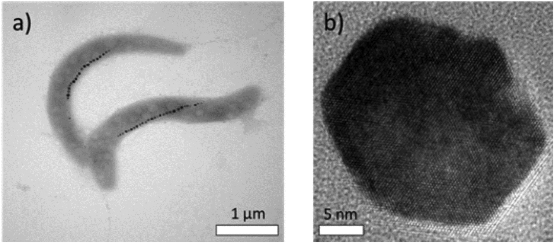 | ||
| Fig. 1 TEM image of (a) Magnetospirillum gryphiswaldense showing chains of magnetosomes, and (b) HRTEM image of a single magnetosome. | ||
In a previous work,30 we observed that the chain, rather than forming a straight line as has been often assumed, presents a slightly bent helical-like configuration. In that work, we showed that the key point to understand that configuration was the 20° tilting of the magnetic moment of each magnetosome out of chain axis, which corresponds to the [111] easy axis of magnetite. We associated this tilting to the presence of an effective uniaxial magnetic anisotropy in that direction, resulting from the competition between the intrinsic magnetocrystalline anisotropy of magnetite and an additional uniaxial shape anisotropy.30 However, the origin of this shape anisotropy was neither discussed nor linked to the particular morphology of magnetosomes.
In the present work, we aim to answer this question by revealing the real morphology of magnetosomes and developing a model to calculate their shape anisotropy energy. We will show, by using electron cryotomography images, that the magnetosomes are not ideal truncated octahedrons but slightly elongated ones. Specifically, they display a ≈7.5% extrusion of one of the {001} square faces and a ≈10% extrusion of an adjacent {111} hexagonal face. Considering these results, we have developed a model based on finite element methods to calculate the magnetostatic energy of these magnetosomes, determining in this way their shape anisotropy. Finally, we have used these results to simulate, in the framework of the Landau–Lifshitz–Gilbert (LLG) equation, the experimental hysteresis loops measured under an external AC field for Magnetospirillum gryphiswaldense dispersed in water.
Experimental methods
Magnetotactic bacteria culture and magnetosome isolation
Magnetospirillum gryphiswaldense MSR-1 (DMSZ 6631) was grown without shaking at 28 °C in an iron rich medium.31 After 96 hours of incubation, once bacteria present well-formed magnetosome chains, the cells were fixed with 2% glutaraldehyde, harvested by centrifugation, and finally suspended in Milli-Q water. Magnetosomes were isolated following the protocol described by Grünberg et al.32 with minor modifications. The cells suspended in 20 mM HEPES-4 mM EDTA (pH = 7.4) were disrupted using a French press. Then, magnetic separation was employed to collect the magnetosomes from cell lysate, and afterwards they were rinsed 10 times with 10 mM Hepes-200 mM NaCl (pH = 7.4). Finally, the isolated magnetosomes were suspended in Milli-Q water at a concentration of 20 μg mL−1.Transmission electron microscopy (TEM)
Electron microscopy was carried out on unstained whole bacteria and isolated magnetosomes adsorbed directly onto carbon-coated copper grids. TEM images were obtained with a JEOL JEM-1400 Plus electron microscope working at a voltage of 120 kV. The particle size distribution was analyzed using ImageJ.33 High-resolution TEM (HRTEM) images were obtained with a TITAN3 (FEI) microscope, working at 300 kV. This high-resolution microscope is equipped with a SuperTwin objective lens and a CETCOR Cs-objective corrector from CEOS Company, giving rise to a point to point resolution of 0.08 nm.Electron cryotomography (ECT)
ECT was carried out on whole bacteria and isolated magnetosomes, both mixed with 10 nm Au nanoparticles (Aurion®BSA gold tracer) employed as markers. The mixture was deposited onto a TEM grid and frozen-hydrated following standard methods, using a Vitrobot Mark III (FEI Inc., Eindhoven, The Netherlands).30 The cryotomographic acquisition was performed with a JEM-2000FS/CR field emission gun transmission electron microscope (Jeol, Europe, Croissy-sur-Seine, France) working at 200 kV. Different single-axis tilt series images were acquired using an UltraScan 4000, 4k × 4k CCD camera (Gatan Inc., Pleasanton, CA, USA), over a tilt range of ±64° with 1.5° increments, using the data acquisition software SerialEM.34 CCD Images were collected at a magnification of 25![[thin space (1/6-em)]](https://www.rsc.org/images/entities/char_2009.gif) 000× and a binning factor of 2 (2048 × 2048 pixel micrographs), producing a pixel size of 0.95 nm. The images in each tilt-series were obtained under the same underfocus and low-dose conditions. For the alignment and 3D reconstruction, we used IMOD software.35 We employed the Au markers during the alignment process, and 3D reconstruction was carried out by weight back-projection and using a Simultaneous Iterative Reconstruction Technique (SIRT). The obtained tomograms were visualized with ImageJ33 as a sequence of cross sectional slices in different orientations. Tomograms were then processed using a median filter and visualized as 3D electron density maps using UCSF Chimera software.36
000× and a binning factor of 2 (2048 × 2048 pixel micrographs), producing a pixel size of 0.95 nm. The images in each tilt-series were obtained under the same underfocus and low-dose conditions. For the alignment and 3D reconstruction, we used IMOD software.35 We employed the Au markers during the alignment process, and 3D reconstruction was carried out by weight back-projection and using a Simultaneous Iterative Reconstruction Technique (SIRT). The obtained tomograms were visualized with ImageJ33 as a sequence of cross sectional slices in different orientations. Tomograms were then processed using a median filter and visualized as 3D electron density maps using UCSF Chimera software.36
AC hysteresis loops
AC magnetometry was carried out using a homemade setup.37 Suspensions of bacteria with a total magnetite concentration of 0.15 mgFe3O4 mL−1 dispersed in Milli-Q water were employed for the experiments. The AC field amplitude was tuned between 0 and 400 Oe, and two different AC field frequencies, 300 and 500 kHz, were employed. All the measurements were performed at 25 °C.Results and discussion
Electron cryotomography imaging of magnetosomes
As has been reported in the literature,38 magnesotomes present faceted crystal morphologies. In the case of M. gryphiswaldense, the crystal morphology of the magnetosomes is similar to a truncated octahedron.30,39 As described in Fig. 2a, in this truncated octahedron, the 〈001〉 crystallographic axes define the growth directions of the square faces, while the 〈111〉 crystallographic axes correspond to the hexagonal faces. M. gryphiswaldense aligns the magnetosomes in a chain according to the 〈111〉 crystallographic directions, along the hexagonal faces of the truncated octahedron.38 In this way, the [111] direction defines the so-called chain-axis.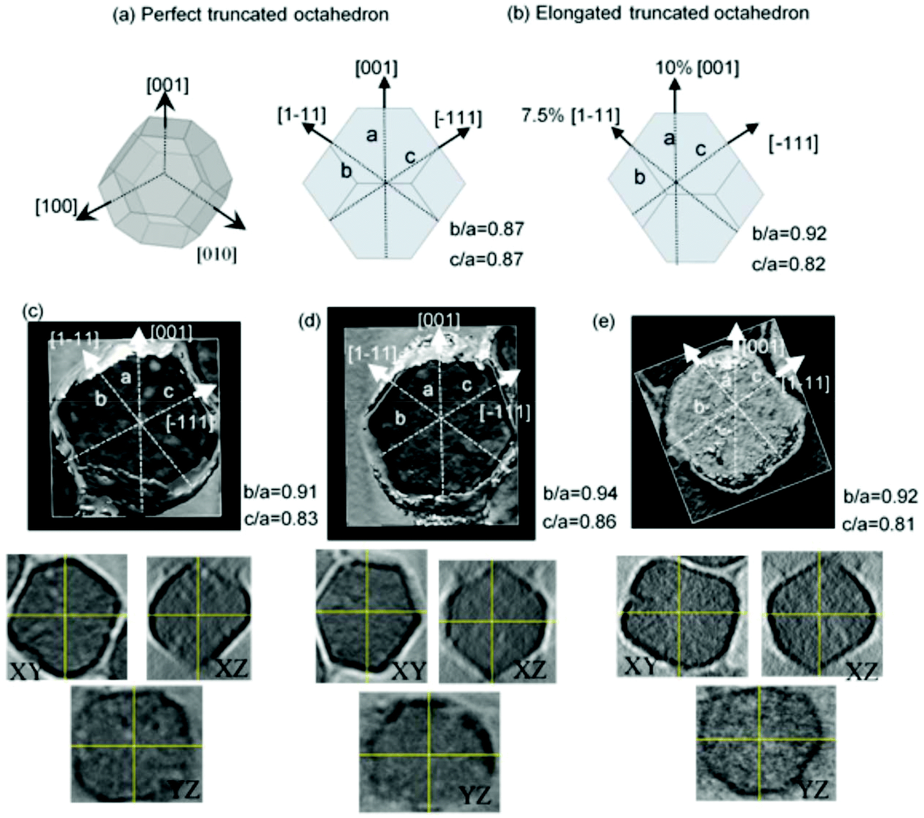 | ||
| Fig. 2 (a) Perfect truncated octahedron. (b) Truncated octahedron with a 10% extrusion along [1–11] direction, and 7.5% extrusion along [001] direction. (c–e) Top: reconstructed 3D tomograms of individual magnetosomes. Bottom: central XY, YZ, and XZ slices of the tomograms shown on top. | ||
From Transmission Electron Microscopy (TEM) images, it is difficult to obtain information about the specific shape details of these nanoparticles with great accuracy. When we deposit magnetosomes onto a copper grid, they can be found in any orientation, which makes hard to know the nanoparticle facet we are working with. In this way, we have employed Electron Cryotomography (ECT) imaging to obtain more reliable information about the actual shape of the magnetosomes. This technique allows us to obtain 3D tomograms of the magnetosomes, thereby revealing any shape deviations these nanoparticles may exhibit. In addition, as we showed in our previous work,30 ECT also provides us with an accurate depiction of the arrangement and spatial configuration of the magnetosomes inside the 3D chain.
As a reference, in Fig. 2a, on the left, we present the 3D geometric shape of a perfect truncated octahedron, and on the right, we show the corresponding 2D projection. In Fig. 2c–e, we present the reconstructed 3D tomograms corresponding to three different magnetosomes. In addition, below them, we also include images of the slices corresponding to the XY, YZ, and XZ planes, which have been used to make the 3D reconstruction. If we compare these 3D tomograms and slices with the geometric shape of a perfect truncated octahedron from Fig. 2a, we observe that the magnetosomes have indeed a faceted morphology similar to the truncated octahedral one, as previously proposed. However, the ECT images suggest that the shape of our magnetosomes does not exactly correspond to a perfect truncated octahedron, since some deformation is observed. As shown in Fig. 2a, this can be checked by measuring the ratio between the distance of two opposing square facets, a, and the distances between two opposing hexagonal facets, either b or c. For a perfect non-deformed truncated octahedron, this ratio should be b/a = c/a = 0.87. By analyzing the 3D reconstructed ECT images of magnetosomes, we have identified the square facets, {001}, and the hexagonal ones {111}, Fig. 2c–e. Once we know the specific facets we are working with, we can measure the corresponding distance ratios along these directions within an error of ≈0.2 nm. As depicted in Fig. 2, for the three magnetosomes we obtain similar ratios: b/a = 0.92(2), and c/a = 0.82(2). This clearly confirms the deviation of the shape of these magnetosomes from a perfect truncated octahedron. Moreover, these experimental ratios can be accurately explained by a combination of ≈7.5% extrusion of one of the {001} square faces and ≈10% extrusion of an adjacent {111} hexagonal face, as shown in Fig. 2b.
Calculation of shape magnetic anisotropy using finite elements method
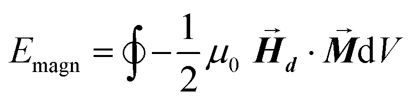
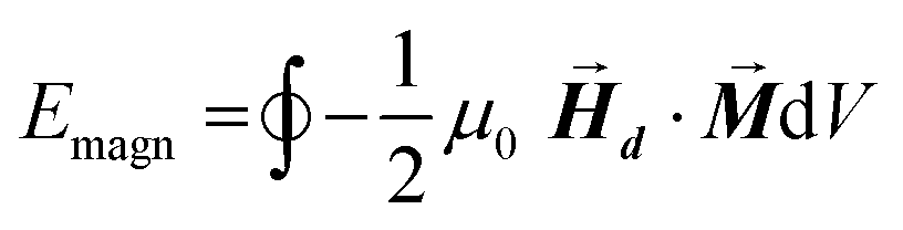
After determining the morphology of the magnetosomes, we have developed a model, using Finite Elements Method (FEM), to calculate the shape magnetic anisotropy associated to that morphology. In general, a rigorous quantitative analysis of the magnetic shape anisotropy of an object requires the calculation of the magnetostatic energy, Emagn, of the given shape, under the constraint that such object is uniformly magnetized in an arbitrary direction.In the simplest case, where the demagnetizing field,  , produced by the magnetization is uniform in the whole object's volume, this magnetostatic energy density is given by:
 | (1) |
This applies only to simple geometries like ellipsoids, where  can be explicitly calculated, and, as can be seen, Emagn is linearly related to the square magnetization by a geometry dependent constant called demagnetizing factor, N.40 If
  is not uniform throughout the volume of the object, eqn (1) transforms to:
 | (2) |
The integral extends to the whole volume of the object and can be numerically calculated by FEM. Just to put the problem into context, it should be recalled that in a typical calculation with macroscopic bodies, the self-demagnetizing action stipulates that magnetization inside the body turns to be non-uniform because the total magnetic field changes from point to point. In contrast, when analyzing single magnetic domain bodies (e.g. magnetic nanoparticles), exchange interaction is assumed to be much higher than Zeeman interaction, so that magnetization can be taken as uniform inside the nanoparticle and free magnetic Poles only exist at the surface. Given that magnetic Poles distribution depends on where the magnetization points to, magnetostatic energy density given by eqn (2) is angle-dependent, and therefore encloses a form of magnetic anisotropy called shape anisotropy.
In the following, we will present the results of performing rigorous numerical calculations of the shape anisotropy in several strongly faceted bodies, and we will mainly focus on the truncated octahedron morphology characteristic of magnetite single crystals such as magnetosomes. Our aim is to show how shape anisotropy is affected by small asymmetries of the original regular morphologies.
To calculate the shape anisotropy energy density for a particular morphology, we follow these basic steps (further details of the model can be found in the ESI)†:
• The magnetization is kept constant along an arbitrary direction given by unit vector ûm,  , where the magnetization module is set as the saturation magnetization of magnetite, M = 480 kA m−1.
• The demagnetizing field  produced by the magnetization is calculated at all points inside the body using FEM.
• For a single magnetization direction, the total magnetostatic energy density is evaluated as:
 | (3) |
• The previous steps are repeated for all orientations of unit vector ûm, that is, the entire solid angle. Unit vector ûm, takes the usual form in spherical coordinates as a function of polar and azimuthal angles (θ, φ):
 | (4) |
This repetition is done in 1° steps, from 0 to 180° for polar angle θ, and from 0 to 360° for azimuthal angle φ.
This simulation has been previously validated in ellipsoids, for which shape anisotropy can be easily calculated.41 Following this procedure, we obtain the energy density landscape, Fig. 3, for different particle morphologies. From the analysis of this landscape, we can determine the easy axes, located at the energy minima, and the anisotropy constants, obtained from the energy barrier between the minima and maxima.
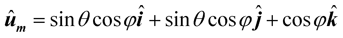
 | ||
| Fig. 3 Magnetostatic energy density of the cube (a), perfect truncated octahedron (b) and perfect octahedron (c). | ||
First, we applied this method for magnetic nanoparticles with regular polyhedral geometry: cubic and octahedral. Truncated octahedral shaped bodies, as our magnetosomes, can be understood as the result of combining a cube and an octahedron in different proportions. Therefore, it is useful to compare the shape anisotropy of these morphologies with the truncated octahedron, which lies midway between both, and is the most probable crystal growing shape for magnetite.42Fig. 3 shows the magnetostatic energy density landscape calculated by eqn (3) for the three mentioned morphologies: cube (C), Fig. 3a, truncated octahedron (TO), Fig. 3b, and octahedron (O), Fig. 3c.
In the case of the cubic morphology, Fig. 3a, the absolute energy minima are located at the 〈111〉 directions, along the cube diagonals, but 6 additional local minima can be found along 〈100〉 directions (perpendicular to square faces), giving a total of 8 + 6 = 14 non-equivalent energy minima or, conversely, 14 easy magnetization axes. Note that in this case the longest dimension is along the diagonal line of the cube. Two anisotropy constants can be calculated, as explained before, from the energy barrier between the absolute 〈111〉 minima and the hard axes 〈110〉, K1 = 5.2 kJ m−3, and between the local 〈100〉 minima and the hard axes 〈110〉, K2 = −52 kJ m−3. The shape anisotropy energy density for the cube, C, can be expressed in terms of the general cubic expansion in powers of the direction cosines of the magnetization,40 taking K1 and K2 as the first and second anisotropy constants.
For the other two regular polyhedrons of Fig. 3, TO and O, the easy axes correspond to the 〈100〉 directions, which are perpendicular to square faces in the TO and along the octahedron vertices in the O. In these cases, only absolute minima are found in 〈100〉 directions. From the energy barrier between these minima and the maxima in 〈111〉 directions, we get an anisotropy constant K1 = 6.7 kJ m−3 for O, and K1 = 1.5 kJ m−3 for TO. As expected, given that the octahedron is strongly non-spherical (higher aspect ratio), the anisotropy constant for the O is much higher than for the TO.
At this point, it must be reminded that TO shape is the basic morphology for magnetosomes of M. gryphiswaldense. Therefore, when magnetocrystalline anisotropy of magnetite, with Kcrys = −11 kJ m−3 and easy axes 〈111〉, is combined with TO shape anisotropy, with Ksh = 1.5 kJ m−3 and easy axes 〈100〉, the magnetosome is, in principle, expected to retain a negative cubic anisotropy character but with reduced energy barriers. However, in real cases, including magnetosomes in bacteria and chemically synthesized magnetite nanoparticles, a magnetic behavior indicative of cubic anisotropy is hardly observed.43 Obviously, non-regular shapes are much more likely in practice, and in this way, the resultant shape anisotropy will end up being uniaxial rather than cubic. The central question is how much “distortion” is needed to overcome the highly symmetric cubic behavior.
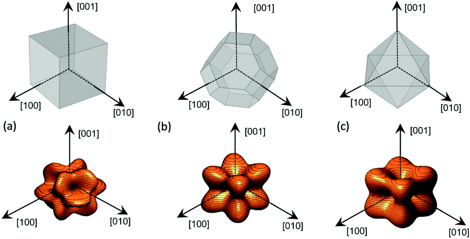
In the case of M. gryphiswaldense, it has been established that each magnetosome in the chain possess its own uniaxial anisotropy, with a well-defined easy axis that should be oriented close to the chain direction, in order to maximize the chain net magnetic moment.30,44,45 Given that the chain axis direction corresponds with the crystallographic 〈111〉 direction of each magnetosome, the first option to analyze the effect of the distortion is to explore what happens to the shape anisotropy energy landscape when lengthening one of the hexagonal faces 〈111〉 of a TO. To this purpose, we have calculated the surface energy for a TO in which one of the hexagonal faces is progressively extruded while keeping the relative orientation of all faces unchanged, Fig. 4a. Moreover, in order to show the shape anisotropy evolution of an extruded TO, we have lengthened one of the hexagonal faces, from 0.5% to 15% of its original size. The corresponding energy landscapes are represented in Fig. 4c.
 | ||
| Fig. 4 (a) Truncated octahedron with an extrusion directed along the [1–11] direction. (b) Linear relationship between the elongation and the shape anisotropy constant. (c) Shape anisotropy energy landscape for different extrusion values, from 0.5 to 15%. | ||
As we increase the extrusion along the [1–11] direction, we can clearly see how we move from a cubic energy landscape to a quasi-uniaxial landscape with the energy minima located along the [1–11] axis. As indicated in Fig. 4b, there is a linear relationship between the elongation along the extruded face and the value obtained for the shape anisotropy constant.
At this point, we would like to remark two points: (i) extrusions as small as 2% already give rise to this single easy axis anisotropy. (ii) With increasing extrusion, the energy landscape acquires a toroidal-like shape, which would in principle suggest uniaxial anisotropy, but the cubic contribution to the shape anisotropy cannot be neglected, and hence we are referring to it as a quasi-uniaxial anisotropy. Therefore, the calculated shape anisotropy energy density for a deformed TO can be approximated to the next analytical function:
 | (5) |
 . The first term corresponds to the uniaxial anisotropy related to the extrusion in the direction of û (in this case û is along the [1–11] direction), and the second term corresponds to the underlying cubic anisotropy, characteristic of the un-extruded TO, being Ksh–c ≈ 1.5 kJ m−3. Depending on how much we elongate the nanoparticle, Ksh–u can take different values as shown in Fig. 4b.
However, as we saw before, ECT images suggest that magnetosomes present 2 extrusions: ≈7.5% extrusion of one of the {001} square faces and ≈10% extrusion of an adjacent {111} hexagonal face, as depicted in Fig. 5a. The shape anisotropy energy of this twice-elongated polyhedron can be calculated by the previously described FEM model, using eqn (3). In this case, as shown in Fig. 5b, the effective quasi-uniaxial easy axis lies near 20° tilted from the [1–11] direction (this would be the direction of û), and the shape anisotropy constant values are Ksh–u = 7 kJ m−3 and Ksh–c = 1.5 kJ m−3.
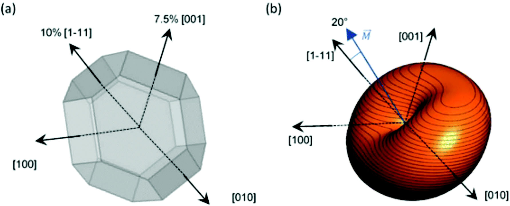 | ||
| Fig. 5 (a) Truncated octahedron with 10% extrusion directed along [1–11] and 7.5% along the [001] direction. (b) Shape anisotropy energy density landscape of the magnetosome system calculated by FEM method. | ||
Therefore, using our FEM model, we have shown that this deformation can in principle explain the 20° tilting of the magnetization vector observed in our previous work. It is difficult to assure the exact way in which the magnetosome is biomineralized so that the chain structure is formed, but what is certain is that, during the biomineralization process, the M. gryphiswaldense bacteria stretch two of its faces to generate a magnetic anisotropy that tilts out the magnetic moment, facilitating in this way the subsequent formation of the helical magnetosome chain in M. gryphiswaldense.30
Hysteresis loops simulation
Finally, we have used the analytical expression obtained for the shape anisotropy energy density, eqn (5), to reproduce the experimental hysteresis loops, M vs. H, of the magnetosome chain inside bacteria (further details of the FEM model employed can be found in the ESI†). In particular, we have applied our model to simulate high frequency AC hysteresis loops of M. gryphiswaldense dispersed in water and measured at 25 °C. These AC hysteresis loops are particularly interesting for magnetic hyperthermia applications, in which the heating efficiency of the nanoparticles is essentially controlled by the area of the AC hysteresis loops described by the magnetic moments of nanoparticles during hyperthermia treatment. In our recent work, we have proven that the biological structure of the chains of magnetosomes is ideal to maximize the hyperthermia efficiency.46 Thanks to the magnetotaxis, when applying a magnetic field, bacteria suffer a torque getting oriented in water. When the bacteria are parallel to the magnetic field, the AC hysteresis loops reach a nearly squared shape, Fig. 6, thereby maximizing the hysteresis loses and the heating efficiency.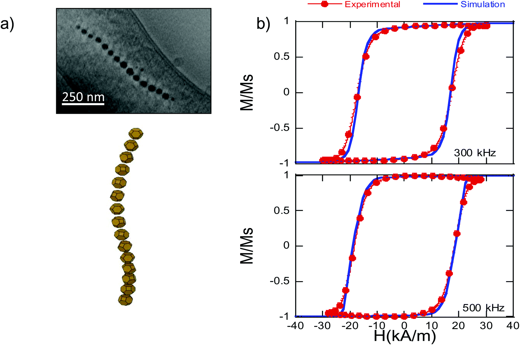 | ||
| Fig. 6 (a) Up: ECT image and down: 3D reconstruction of the chain of magnetosomes of M. gryphiswaldense30 − Published by The Royal Society of Chemistry. (b) AC hysteresis loops, M vs. H, measured at 300 and 500 kHz for bacteria dispersed in water (25 °C), and simulated hysteresis loops using eqn (6) and (7). | ||
In this context, the chain of magnetosomes, each of which has a particular magnetic shape anisotropy, can be approximated to a 1D assembly of single magnetic domains. The energy density landscape of the individual magnetosomes can be reduced to:
 | (6) |
The first term, Ecrys, corresponds to the magnetocrystalline anisotropy energy density of magnetite, and is given by the typical cubic anisotropy expression. Since magnetosomes are pure magnetite crystals, we have used the expected bulk value for the magnetocrystalline anisotropy constant Kcrys = −11 kJ m−3.40 The second term, Eshape, corresponds to the shape anisotropy energy density of the magnetosome according to eqn (5), being Ksh–u = 7 kJ m−3 and Ksh–c = 1.5 kJ m−3 as we explained before. In this case, ûm,i is the unit vector director of the magnetization  , and û corresponds with the direction of effective quasi-uniaxial easy axis, which lies 20° tilted from the [1–11] direction, as explained before. The third term, Edip, corresponds to dipolar energy due to interactions between magnetosomes inside the chain. Electron cryotomography allow us to determine the XYZ positions and relative orientations of each magnetosome inside the chain, see Fig. 6a. In this third term, âij is the unit vector along the line joining particles i and j, located at a distance given by a = 60 nm, and V = 381 103 nm3 is the volume of each particle, considering a mean size of 45 nm, the same for all for simplicity, see Fig. 6a. Finally, the last term, EZeeman, corresponds to the Zeeman energy, where H is the alternating AC magnetic field.
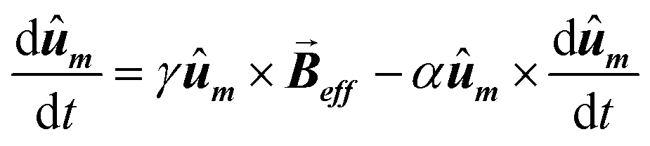
Then, the AC hysteresis loops can be modeled solving the quite general Landau–Lifshitz–Gilbert equation for the magnetization dynamics of a single domain subjected to an arbitrary effective field, 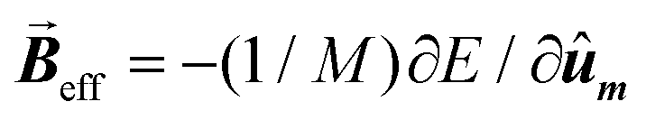 :
:
 | (7) |
In this equation α = 0.05 is the so-called Gilbert damping constant (dimensionless constant),47,48γ = 2 is the gyromagnetic ratio of free electron,  is the magnetization, and E is the energy density of a single nanoparticle. Some limitations should be noted. In this model thermal fluctuations are completely neglected (T = 0 K), so it is expected to work fine when magnetization is anchored to energy minima. In our case, since magnetosomes are particles with a mean size ∼45 nm, the anisotropy energy, KV, is much higher than the thermal energy, kBT, at 25 °C, and, consequently, the magnetization is strongly anchored to energy minima. Moreover, as we work with energy densities, the volume of particles only enters explicitly the LLG model through the dipolar interactions, so this approach is mostly size-insensitive.
In Fig. 6b, we show the experimental AC hysteresis loops of bacteria dispersed in water, measured at 300 and 500 kHz, and the simulated hysteresis loops, using eqn (6) and (7). As can be observed, in both cases, the simulated hysteresis loops nearly overlap the experimental ones, indicating that the model we have developed to determine the shape anisotropy energy landscape allows us to reproduce the magnetic behavior of the chain of magnetosomes in M. gryphiswaldense. Moreover, these good initial results open the possibility of extrapolating our model to calculate the shape anisotropy of other highly faceted magnetic nanoparticles.
Conclusions
In this work we have proven that shape anisotropy plays a crucial role in the configuration and magnetic behavior of faceted nanoparticles, such as magnetosomes synthesized by M. gryphiswaldense. The shape anisotropy energy density for a particular morphology of the nanoparticle can be calculated using a Finite Element Methods approach. In the case of magnetosomes, their morphology has been analyzed by using electron cryotomography, revealing that it slightly deviates from a perfect truncated octahedron, due to ≈7.5% extrusion of one of the {001} square faces and ≈10% extrusion of an adjacent {111} hexagonal face. This deformation defines the shape anisotropy energy landscape of the magnetosome, with a unique quasi-uniaxial character, arising from the competition between the cubic shape anisotropy associated to the truncated-octahedral shape, and a uniaxial shape anisotropy associated to the deformation. Finally, we have used the analytical expression of the shape anisotropy obtained by finite elements to simulate, within the framework of the Landau–Lifshitz–Gilbert model, the experimental AC hysteresis loops measured for these magnetotactic bacteria at 25 °C. These results indicate that the chain of magnetosomes constitutes a perfect playground to check the importance of shape anisotropy in hierarchical nanostructures, and we hope these results will help other groups to better understand the importance of shape anisotropy in the development of their nanostructures for all types of applications.Conflicts of interest
There are no conflicts to declare.Acknowledgements
Spanish Government is acknowledged for funding under the project number MAT2017- 83631-C3. Basque Government is acknowledged for funding under the project number IT1245-19. HRTEM images were obtained in the Laboratorio de Microscopias Avanzadas at Instituto de Nanociencia de Aragón – Universidad de Zaragoza (LMA-INA). Authors acknowledge the LMA-INA for offering access to their instruments and expertise. Authors thank Prof. J. A. García and I. Rodrigo for providing AC hysteresis loops.References
- D. Lisjak and A. Mertelj, Prog. Mater. Sci., 2018, 95, 286–328 CrossRef CAS.
- H. Khurshid, J. Alonso, Z. Nemati, M. H. Phan, P. Mukherjee, M. L. Fdez-Gubieda, J. M. Barandiarán and H. Srikanth, J. Appl. Phys., 2015, 117, 17A337 CrossRef.
- R. H. Kodama, J. Magn. Magn. Mater., 1999, 200, 359–372 CrossRef CAS.
- G. F. Dionne, in Magnetic Oxides, ed. G. F. Dionne, Springer, New York, 2009, pp. 201–271 Search PubMed.
- M. E. Mchenry, D. E. Laughlin, M. Science and C. Mellon, Magnetic Properties of Metals and Alloys, Elsevier, 2014, vol. 1 Search PubMed.
- Ò. Iglesias, A. Labarta, U. De Barcelona and I. Introduction, Phys. Rev. B: Condens. Matter Mater. Phys., 2001, 63, 184416 CrossRef.
- J. Restrepo, Y. Labaye and J. M. Greneche, Physica B: Condens. Matter, 2006, 384, 221–223 CrossRef CAS.
- H. Gojzewski, M. Makowski, A. Hashim, P. Kopcansky, Z. Tomori and M. Timko, Scanning, 2012, 34, 159–169 CrossRef CAS.
- J. Mazo-Zuluaga, J. Restrepo and J. Mejía-López, Physica B: Condens. Matter, 2007, 398, 187–190 CrossRef CAS.
- H. Kachkachi, A. Ezzir, M. Noguès and E. Trouc, Eur. Phys. J. B, 2000, 14, 681–689 CrossRef CAS.
- J. Mazo-Zuluaga, J. Restrepo and J. Mejía-López, J. Appl. Phys., 2008, 103, 113906 CrossRef.
- R. H. Kodama and A. E. Berkowitz, Phys. Rev. B: Condens. Matter Mater. Phys., 1999, 59, 6321–6336 CrossRef CAS.
- J. L. Dormann, D. Fiorani and E. Tronc, J. Magn. Magn. Mater., 1999, 202, 251–267 CrossRef CAS.
- M. F. Hansen and S. Mørup, J. Magn. Magn. Mater., 1998, 184, L262–L274 CrossRef.
- R. Moreno, S. Poyser, D. Meilak, A. Meo, S. Jenkins, V. K. Lazarov, G. Vallejo-Fernandez, S. Majetich and R. F. L. Evans, Sci. Rep., 2020, 10, 2722 CrossRef CAS.
- G. Singh, H. Chan, A. Baskin, E. Gelman, N. Repnin, P. Král and R. Klajn, Science, 2014, 345, 1149–1153 CrossRef CAS PubMed.
- E. Alphandéry, Front. Bioeng. Biotechnol., 2014, 2, 5 Search PubMed.
- Z. Nemati, J. Alonso, I. Rodrigo, R. Das, E. Garaio, J. Á. García, I. Orue, M. H. Phan and H. Srikanth, J. Phys. Chem. C, 2018, 122, 2367–2381 CrossRef CAS.
- I. Castellanos-Rubio, I. Rodrigo, R. Munshi, O. Arriortua, J. S. Garitaonandia, A. Martinez-Amesti, F. Plazaola, I. Orue, A. Pralle and M. Insausti, Nanoscale, 2019, 11, 16635–16649 RSC.
- J. Lee and S. H. Ko, in Hierarchical Nanostructures for Energy Devices, 2014, pp. 7–25 Search PubMed.
- R. P. Blakemore, Annu. Rev. Microbiol., 1982, 36, 217–238 CrossRef CAS PubMed.
- R. E. Dunin-borkowski, M. R. Mccartney, R. B. Frankel, D. A. Bazylinski, M. Posfai and P. R. Buseck, Science, 1998, 282, 1868–1870 CrossRef CAS PubMed.
- D. Faivre and D. Schüler, Chem. Rev., 2008, 108, 4875–4898 CrossRef CAS PubMed.
- K. Grünberg, E. C. Müller, A. Otto, R. Reszka, D. Linder, M. Kube, R. Reinhardt and D. Schüler, Appl. Environ. Microbiol., 2004, 70, 1040–1050 CrossRef PubMed.
- A. Scheffel, M. Gruska, D. Faivre, A. Linaroudis, J. M. Plitzko and D. Schüler, Nature, 2006, 440, 110–114 CrossRef CAS PubMed.
- E. Katzmann, A. Scheffel, M. Gruska, J. M. Plitzko and D. Schüler, Mol. Microbiol., 2010, 77, 208–224 CrossRef CAS.
- O. Draper, M. E. Byrne, Z. Li, S. Keyhani, J. C. Barrozo, G. Jensen and A. Komeili, Mol. Microbiol., 2011, 82, 342–354 CrossRef CAS.
- D. Schu, A. Scheffel and D. Schüler, J. Bacteriol., 2007, 189, 6437–6446 CrossRef PubMed.
- A. G. Meyra, G. J. Zarragoicoechea and V. A. Kuz, Phys. Chem. Chem. Phys., 2016, 18, 12768–12773 RSC.
- I. Orue, L. Marcano, P. Bender, A. García-Prieto, S. Valencia, M. A. Mawass, D. Gil-Cartón, D. Alba Venero, D. Honecker, A. García-Arribas, L. Fernández Barquín, A. Muela and M. L. Fdez-Gubieda, Nanoscale, 2018, 10, 7407–7419 RSC.
- U. Heyen and D. Schüler, Appl. Microbiol. Biotechnol., 2003, 61, 536–544 CrossRef CAS.
- K. Grünberg, C. Wawer, B. M. Tebo and D. Schuler, Appl. Environ. Microbiol., 2001, 67, 4573–4582 CrossRef PubMed.
- J. Schindelin, C. T. Rueden, M. C. Hiner and K. W. Eliceiri, Mol. Reprod. Dev., 2015, 82, 518–529 CrossRef CAS PubMed.
- D. N. Mastronarde, J. Struct. Biol., 2005, 152, 36–51 CrossRef PubMed.
- J. R. Kremer, D. N. Mastronarde and J. R. McIntosh, J. Struct. Biol., 1996, 116, 71–76 CrossRef CAS PubMed.
- E. F. Pettersen, T. D. Goddard, C. C. Huang, G. S. Couch, D. M. Greenblatt, E. C. Meng and T. E. Ferrin, J. Comput. Chem., 2004, 25, 1605–1612 CrossRef CAS PubMed.
- E. Garaio, J. M. Collantes, F. Plazaola, J. A. Garcia and I. Castellanos-Rubio, Meas. Sci. Technol., 2014, 25, 115702 CrossRef.
- S. Mann, R. B. Frankel and R. P. Blakemore, Nature, 1984, 310, 405–407 CrossRef.
- L. Marcano, A. García-Prieto, D. Muñoz, L. Fernández Barquín, I. Orue, J. Alonso, A. Muela and M. L. Fdez-Gubieda, Biochim. Biophys. Acta, Gen. Subj., 2017, 1861, 1507–1514 CrossRef CAS PubMed.
- B. D. Cullity and C. D. Graham, Introduction to Magnetic Materials (2nd Edition), 2009, vol. 12 Search PubMed.
- D. X. Chen, E. Pardo and A. Sanchez, IEEE Trans. Magn., 2002, 38, 1742–1752 CrossRef.
- Y. Xia, Y. Xiong, B. Lim and S. E. Skrabalak, Angew. Chem., Int. Ed., 2009, 48, 60–103 CrossRef CAS PubMed.
- N. A. Usov and J. M. Barandiarán, J. Appl. Phys., 2012, 112, 053915 CrossRef.
- S. Mann, T. T. Moench and R. J. P. Williams, Proc. R. Soc. London, Ser. B, 1984, 221, 385–393 CAS.
- A. Körnig, M. A. Hartmann, C. Teichert, P. Fratzl and D. Faivre, J. Phys. D: Appl. Phys., 2014, 47, 235403 CrossRef.
- D. Gandia, L. Gandarias, I. Rodrigo, J. Robles-García, R. Das, E. Garaio, J. Á. García, M. H. Phan, H. Srikanth, I. Orue, J. Alonso, A. Muela and M. L. Fdez-Gubieda, Small, 2019, 15, 1902626 CrossRef CAS PubMed.
- E. Barati and M. Cinal, Phys. Rev. B, 2017, 95, 134440 CrossRef.
- W. T. Coffey, D. S. F. Crothers, J. L. Dormann, Y. P. Kalmykov, E. C. Kennedy and W. Wernsdorfer, Phys. Rev. Lett., 1998, 80, 5655–5658 CrossRef CAS.
Footnote |
| † Electronic supplementary information (ESI) available: Detailed description of the finite element ethods model employed to simulate the shape anisotropy energy landscape. See DOI: 10.1039/d0nr02189j |
| This journal is © The Royal Society of Chemistry 2020 |