
Short period sinusoidal thermal modulation for quantitative identification of gas species†
Aijun
Yang‡
a,
Jifeng
Chu‡
 a,
Weijuan
Li‡
a,
Dawei
Wang
a,
Xu
Yang
a,
Tiansong
Lan
a,
Xiaohua
Wang
*a,
Mingzhe
Rong
*a and
Nikhil
Koratkar
*bc
a,
Weijuan
Li‡
a,
Dawei
Wang
a,
Xu
Yang
a,
Tiansong
Lan
a,
Xiaohua
Wang
*a,
Mingzhe
Rong
*a and
Nikhil
Koratkar
*bc
aState Key Laboratory of Electrical Insulation and Power Equipment, Xi'an Jiaotong University, Xi'an 710049, PR China. E-mail: xhw@mail.xjtu.edu.cn; mzrong@mail.xjtu.edu.cn
bDepartment of Mechanical, Aerospace and Nuclear Engineering, Rensselaer Polytechnic Institute, Troy, NY 12180, USA
cDepartment of Materials Science and Engineering, Rensselaer Polytechnic Institute, Troy, NY 12180, USA. E-mail: koratn@rpi.edu
First published on 12th November 2019
Abstract
The field of chemical (gas) sensing has witnessed an unprecedented increase in device sensitivity with single molecule detection now becoming a reality. In contrast to this, the ability to distinguish or discriminate between gas species has lagged behind. This is problematic and results in a high rate of false alarms. Here, we demonstrate a short period sinusoidal thermal modulation strategy to quantitatively and rapidly identify two industrially relevant gases (hydrogen sulfide (H2S) and sulfur dioxide (SO2)) by using a single semiconducting metal oxide sensor device. By applying sinusoidal heating voltages with a fixed short period, we were able to simultaneously obtain distinct patterns of dynamic responses. These characteristic patterns were adopted to build and validate a gas recognition library. Our approach does not rely on large-scale sensor arrays and complex algorithms and is amenable for real-time and low-power gas monitoring.
Introduction
Hydrogen sulfide (H2S) and sulfur dioxide (SO2) are both toxic gas species and threatening to human health even at the level of parts per million (ppm).1 In addition, they are typical decomposition products of sulfur hexafluoride (SF6). Types and contents of H2S and SO2 in SF6-based electrical equipment can be used as indicators to reflect the running state of equipment.2–6 Therefore, the detection of H2S and SO2 has become an essential need for both human safety and power system health monitoring. Traditional methods to monitor these gases are based on optics, including differential optical absorption spectroscopy (DOAS),7 Fourier transform infrared spectroscopy (FTIR),8 and quartz-enhanced photoacoustic spectroscopy (QEPAS).9 All of the above methods require complex designed structures while incurring high cost and are not suitable for onsite monitoring in the field. Recently, gas sensors based on transition metal oxides (TMOs) have attracted much attention due to their low cost, miniaturization and easy integration.10–13 Various sensors have been developed to “separately” detect H2S and SO2 using TMOs.14,15 However, such sensors exhibit very poor ability to distinguish between these gases because of the sensors’ cross-sensitivity to multiple gases.To address the problem of cross-sensitivity, Hu et al.16 have proposed a method of rotational–vibrational modes based on graphene plasmons to identify various gas molecules (SO2, NO2, N2O, and NO), which was similar to in situ experiments. Furthermore, various adsorption mechanisms between gas molecules and sensing materials were also demonstrated. However, all gas concentrations they tested exceeded 1000 ppm, and it is unknown whether the method is suitable for low concentrations. Apart from the above method, sensor arrays combined with pattern recognition software have also been widely used to identify different gases. Through the use of neural network technology, Zhang et al.17 have investigated sensor arrays to quantitatively distinguish formaldehyde and NH3 at a concentration from 5 to 100 ppm. Along similar lines, a hybrid multisensory system was presented by De Vito et al.18 for investigating the quantification of NO2 (from 0 to 900 ppb), NH3 (from 0 to 20 ppm) and humidity (ranging from 30 to 60%). Thus, sensor arrays can realize multi-gas identification, but at the expense of increased complexity, cost, sensor size/power, and the need for complex pattern recognition algorithms such as neural networks or machine learning, which further increases the device complexity.
Exploiting the temperature dependent response of the sensor is another viable strategy to recognize different gases. Wu et al.19 have utilized characteristic sensor response patterns versus temperature to discriminate gases, but this approach requires several response versus temperature curves to be generated, making real-time monitoring a challenge. Some noteworthy efforts at the dynamic thermal modulation of the sensor have also been carried out. For example, in ref. 20, the heating voltage applied to the sensor was changed slowly to obtain multiple quasi-steady states. However, this is essentially equivalent to operation at different steady-state temperatures, which again makes rapid (real-time) detection difficult to accomplish. Furthermore, the average sensor temperatures were of the order of 300 °C,20 which greatly increased the power consumption of the device.
A virtual sensor array has become a research hotspot due to its ability to acquire lots of experimental data quickly with less sensors. Li et al.21 set one sensor to continuously scan and record the amplitude information of the acoustic signal of gas leakage, to simulate several sensors working at different positions for locating the gas leakage. They achieved high precision results on gas leakage localization. Zeng et al.22 took a single-chip temperature compensated film bulk acoustic wave resonator coated with 20-bilayer self-assembled poly(sodium 4-styrenesulfonate)–poly(diallyldimethylammonium chloride) thin films to form a virtual sensor array used for the discrimination of six different volatile organic compounds. They employed a microcontroller to modulate temperature, which makes the virtual sensor array easy to integrate. However, their study suffered from long test cycle (about 10-minute per cycle), and could only achieve gas type identification, but not the quantitative detection of gases, which limits its industrial applications.
Another key point is that previous attempts at distinguishing between gases have proven successful with gases that differ significantly in their chemical characteristics. For the accurate discrimination of H2S and SO2, there have been a few literature studies reported. Previous literature23–25 indicated that the reported gas sensors employed to detect H2S and SO2 exhibited strong cross-sensitivity, thus TMO-based gas detectors cannot quantitatively distinguish gas concentrations only depending on response values.
In this work, we show that one can quantitatively discriminate between H2S and SO2 by using a “single” semiconducting transition metal oxide (i.e., Au doped CeO2) sensor device. We demonstrate that by introduction of short period sinusoidal heating modulation, the sensor can be operated thermo-cyclically (Fig. S1†). Periodic sampling at “eight” fixed points during one cycle simultaneously yields “eight” distinct dynamic response curves, which were used as characteristic patterns to build a gas recognition library, that could be used to establish the identity and concentration of the gas being detected, without the need for sensor arrays or complex pattern recognition algorithm. Moreover, this approach enabled us to rapidly acquire the sensor dynamic response at different temperatures using a “single” sensor device and in just “one” test cycle. In other words, one sensor working at the sinusoidal heating voltage is equivalent to eight virtual sensors simultaneously working at different heating voltages. Although this work has focused on the identification of H2S and SO2, the approach presented here is generic, and could, in principle, be extended to other relevant gas species.
Results and discussion
The materials and protocols used to synthesize semiconducting thin films of ceria (CeO2) nanoparticles (NPs) and Au-doped CeO2 NPs are provided in the Experimental section. Microscopic and spectroscopic characterization of the pristine CeO2 film and the Au-doped CeO2 films is provided in Fig. S2.† The crystal structure of the samples was confirmed using X-ray diffraction (XRD), which indicated (Fig. S2a†) several prominent peaks that correspond to the (111), (200), (220), (311), (222), (400), (331) and (420) crystal planes of CeO2 (JCPDS no. 81-0792).26 For the Au-doped film, a diffraction peak is also observed at 2θ of 38.1°, which is attributed to the (111) plane of Au.27 Fig. S2b† presents the Raman spectra of CeO2 NPs and its doped counterpart. CeO2 exhibits a prominent Raman peak near 461 cm−1 due to the F2g Raman active mode of the fluorite structure.28 The introduction of Au dopants has no significant effect on the location of the CeO2 Raman peaks. Scanning electron microscopy (SEM) was used to analyse the morphology of the pristine and functionalized CeO2 NPs. The image of the pristine CeO2 shows NPs which have randomly aggregated (Fig. S2c†). However, the Au-doped CeO2 NPs in Fig. S2d† appear to self-assemble into flakes with a diameter of ∼2 μm, which might be ascribed to the introduction of HAuCl4 (Methods) that changed the pH value of the dispersion. Such lamellar structures are known to be more conducive to the diffusion and adsorption of gas molecules, thereby enhancing the gas-sensing properties.29,30 The EDS (point scan) of products is presented in Fig. S3,† in which Ce, O, and a noble metal element (i.e., Au) can be observed, which confirms successful Au doping. Furthermore, the EDS results indicated that the doping ratio of Au is near the theoretical doping ratio of ∼4.5%. Fig. S4a† shows the STEM image of Au–CeO2 nanosheets in the dark field and the combination of all the elements. Fig. S4b–S4d† individually shows four elemental mappings of Ce, O, and Au. Notably, the mapping of Ce and the mapping of O basically coincide in shape and size, which means that the element O is totally ascribed to the O in the CeO2 NPs. Besides, we can see that the green particles distributed on the surface of CeO2 are Au NPs. The energy dispersive spectrometer spectrum (EDS, mapping scan) of products is shown in Fig. S5,† in which only Ce, O, and Au elements can be observed. The Cu peak is derived from the micro-grid copper mesh; thus, it could be ignored. Furthermore, we have analysed the mass ratio and atomic ratio of elements in the STEM of the Au–CeO2 sample, and found that it is roughly consistent with the EDS in Fig. S3.† The morphology of Au–CeO2 was characterized by typical transmission electron microscopy (TEM) and can be seen in Fig. 1a. The size of Au NPs is measured at 41.13 nm, which demonstrates that Au NPs are nano-scale (Fig. 1b). Besides, the size of CeO2 NPs is in the range of 5–20 nm, but most of them are agglomerated into large flakes, as we can see in Fig. S2d.† To further investigate the microstructure of Au–CeO2, high-resolution TEM (HRTEM) images are recorded as shown in Fig. 1c and d. The lattice spacing of 0.321 nm corresponds to the distance between the (111) lattice planes of CeO2. Furthermore, the Au particles show a well crystalline structure with a lattice spacing of 0.224 nm that can be ascribed to the (111) planes.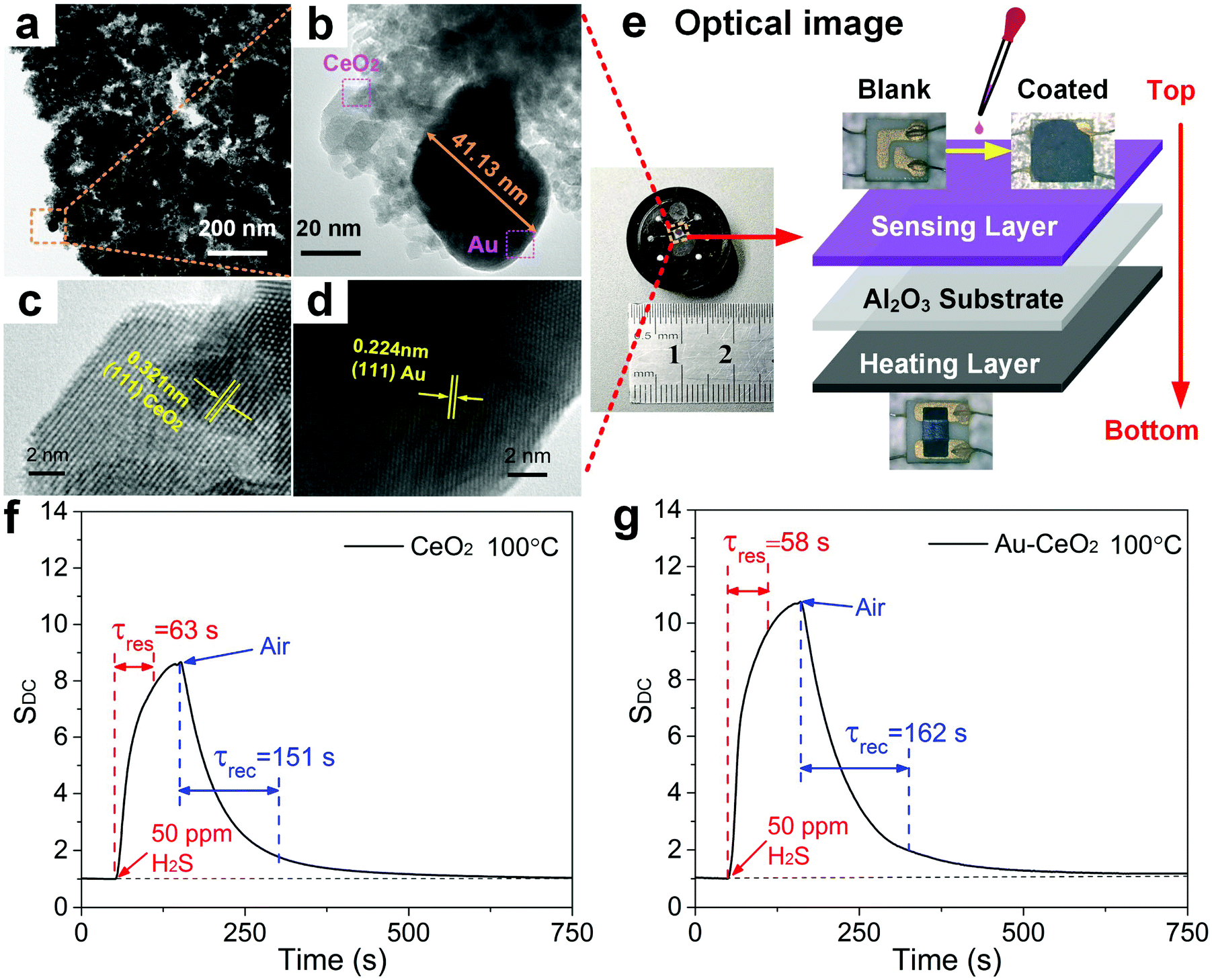 | ||
| Fig. 1 Semiconducting metal oxide gas sensor and its typical response to H2S. (a) TEM image of Au–CeO2. (b) Partial enlargement of (a). HRTEM images of (c) CeO2 NPs and (d) Au NPs. SEM image of Au–CeO2 and its local magnification. (e) Optical image and schematic illustration of the sensor. The response–recovery curves of (f) CeO2, (g) Au–CeO2 for sensing 50 ppm H2S at 100 °C. | ||
The Au–CeO2 sensor structure is shown in Fig. 1e. The sensor is constituted by three layers, in which the top layer is composed of the gas responsive film. Alumina is utilized as the intermediate layer due to its excellent electrical insulation properties. Finally, the bottom layer is composed of a ruthenium oxide heater, which provides the needed temperature. From the inset of Fig. 1e, it is evident that the sensor device is fairly compact. Fig. 1f and g show the typical responses of the CeO2 and Au–CeO2 sensors respectively, when exposed to ∼50 ppm H2S at a temperature of ∼100 °C. At a direct current (DC) heating voltage, the response of the sensor is defined as follows:
| SDC = Ig\_DC/Ia\_DC | (1) |
In order to understand the role of Au doping on gas interaction with ceria (CeO2) based sensors, we studied the adsorption of H2S and SO2 on pure ceria (111) and Au doped ceria (111) using density functional theory calculations corrected by on-site Coulomb interactions (DFT+U). The results of H2S adsorbed on ceria are discussed here. After structural optimization, the most stable configurations are shown in Fig. S6.† The values of adsorption energy (Eads), the nearest distance (dgas–ceria) between the gas molecule and substrate, charge transfer (Q) and work function modification (ΔΦ) are all listed in Table S1 in the ESI.† The results in Fig. S6a† indicate that H2S is physically adsorbed on the pure ceria surface, with 0.0025e electrons transferring to the substrate. In contrast, Fig. S6b† shows S–Au bond formation between the H2S molecule and Au–ceria surface, indicating chemical adsorption. In addition, the Eads of H2S adsorbed on the Au–ceria surface (−2.175 eV) is much larger than that of H2S adsorbed on the baseline ceria surface (−0.424 eV), and the charge transfer follows the same order, with 0.2126e electrons transferring to Au–ceria during adsorption. Therefore, the role of the Au dopant atoms is to facilitate enhanced H2S adsorption on the CeO2. Furthermore, Fig. S6c† shows that the 2p orbital of H2S contributes towards adsorption on pure ceria as indicated by the obvious peak of the PDOS near the Fermi level. However, the PDOS curve does not fluctuate significantly near the Fermi level in Fig. S6d† (for Au-doped ceria), with the Fermi level of TDOS upshifted when compared with that of pure ceria. The reason for this phenomenon is greater electron transfer from the H2S molecule to the Au–ceria surface when compared to ceria during adsorption. The larger value of ΔΦ for H2S adsorbed on Au–ceria than on ceria in Table S1† is also in accordance with the stronger interaction of the former system. A possible adsorption pathway for H2S on Au-doped ceria in the presence of air (oxygen) is illustrated in Fig. S6e.† The corresponding adsorption results for SO2 on the surface of ceria are shown in Fig. S7 and Table S2.† As before, we find that the adsorption energy is improved by Au doping of the ceria surface and there is greater electron transfer from SO2 to the Au-doped substrate. Based on its superior performance, we decided to utilize the Au–CeO2 sensor for all subsequent work in this study.
To examine the cross-sensitivity of the sensor to H2S and SO2, we utilized the as-prepared Au–CeO2 sensor to measure the response of these two gases at various concentrations at a constant temperature of ∼100 °C (Fig. S8a and b†). As expected, the current change increases with the increase in gas concentration, and the relationship between the response values and gas concentrations are shown in Fig. S8c and d,† where the determination coefficients (R2) are ∼1 indicating good fitting precision. From the fitting curves, it is evident that the response values are overlapped partly, and therefore the detected gases cannot be distinguished based on this information. This shows that a single TMO based sensor operating at a fixed temperature is clearly incapable of discriminating between H2S and SO2, which is consistent with what has been reported in the literature.
As discussed previously, the Au–CeO2 sensing film and ruthenium oxide heating materials are respectively coated on the upper and lower sides of the sensor, and the schematic diagrams are shown in Fig. 2. The Au–CeO2 sensor was operated under a sinusoidal heating mode (Fig. 2b). The period and average value of the heating voltage are ∼8 s and ∼2 V, respectively. The average value of the heating current was ∼60 mA and in-phase with the heating voltage (Fig. S9b†). From this, we can deduce that the power consumption of the sensor is ∼140 mW. The varying surface temperature of the sensor was also monitored by an IR camera (Fig. S10a†). The temperature of the sensing film varies synchronously in the range of ∼60 °C to ∼110 °C with the applied heating current (Fig. S10b†). In Fig. 2a, the sensor current (I) in air, with the sampling period being ∼1 s, also synchronously varies following the heating current and shows good repeatability, which indicates that the device has the potential of long-term stable operation. The sampling current at sampling N (IN) is defined as
| IN = I(t) | (2) |
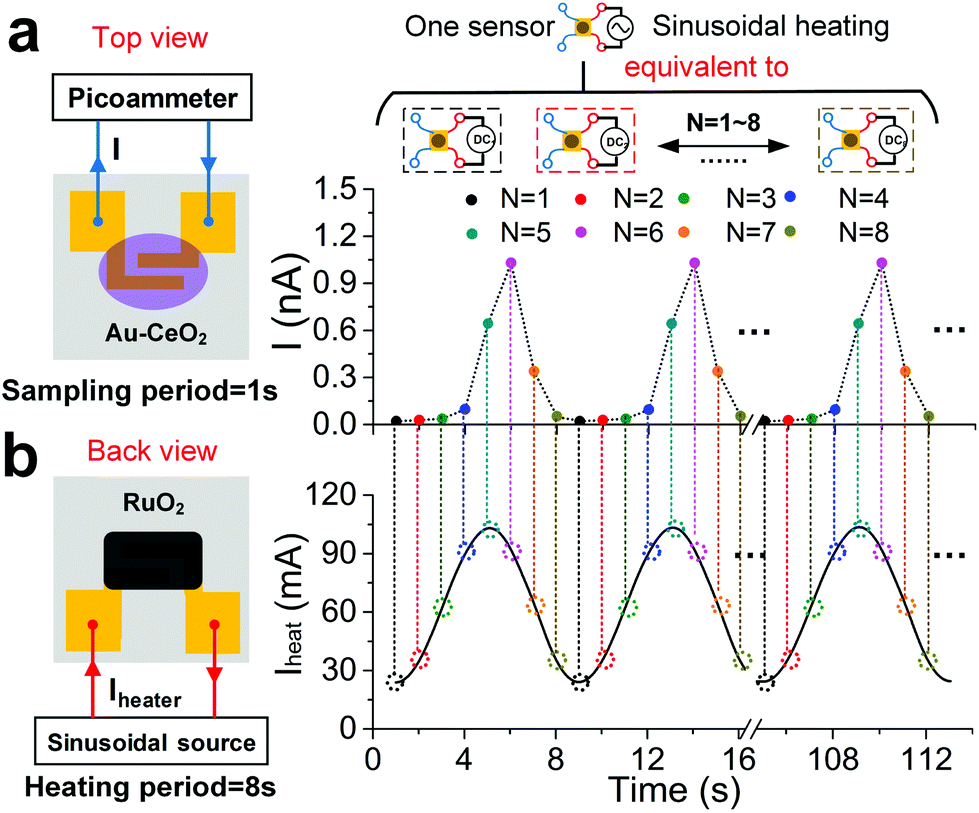 | ||
| Fig. 2 Concept of short period sinusoidal thermal modulation. (a) Top view of the sensitive layer, and the variation of sensor current in air under the sinusoidal heating voltage. (b) Back view of the heating layer, and the variation of heating current through the heater. | ||
The dynamic curves of sensor current for sensing 50 ppm H2S and SO2 are given in Fig. S11a and b.† It is evident that the current curve fluctuates markedly due to the introduction of short period sinusoidal heating modulation. According to the previous definition of IN, the 8-separate sampling current curves are presented in Fig. 3a and b, respectively for H2S and SO2. In this manner, by simply utilizing a single Au–CeO2 sensor device, we can simultaneously acquire distinct patterns of dynamic responses of H2S and SO2. The response times of all IN curves for sensing ∼50 ppm H2S ranged from ∼62 to ∼70 s. Taking the maximum IN curve at N = 6 as an example, the response and recovery times are ∼62 s and ∼198 s, respectively. Similarly, toward ∼50 ppm SO2, the sensor response sampled at N = 6 has a response time and recovery time of ∼98 s and ∼372 s, respectively. Furthermore, response value at sampling N can be defined by
| SN = INg/INa | (3) |
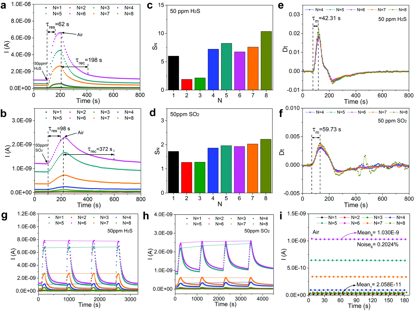 | ||
| Fig. 3 Sensor response to short period sinusoidal thermal modulation. IN of the sensor toward (a) ∼50 ppm H2S and (b) ∼50 ppm SO2 under the sinusoidal thermal modulation. The response values at different sampling N of the sensor toward (c) ∼50 ppm H2S and (d) ∼50 ppm SO2. The derivative curves at different sampling N of the sensor toward (e) ∼50 ppm H2S and (f) ∼50 ppm SO2. The repeatability of the Au–CeO2 sensor upon exposure to (g) ∼50 ppm H2S and (h) ∼50 ppm SO2. (i) Noise assessments of eight IN curves in air. | ||
To obtain more in-depth information of the sensor's response to the detected gas, the time derivative of IN expressed by “Dt” has been introduced in Fig. 3e and f. It should be noted that the shape characteristics of the sensor response curve are encoded in this derivative information. A series of derivative curves (taken at sampling N) jointly contribute to curve clusters. It can be noticed that every curve in the cluster has its maximum point and the time required for a derivative curve to reach its maximum point from zero, is expressed as “τN”. The physical meaning of τN is the time needed for the fastest change of sensor current. Then, the mean of every τN taken at sampling N is represented by “τm”, which can be used as another characteristic for gas recognition. From Fig. 3e and f, it is evident that the shape of the derivative curves is greatly different for ∼50 ppm H2S and SO2, and τm are equal to ∼42.31 s and ∼59.73 s, respectively.
The reproducibility and noise assessment are both significant parameters for evaluating the performance of gas sensors. Fig. 3g and h illustrate four successive response–recovery cycles of IN for the sensor exposed to ∼50 ppm H2S and SO2, respectively. It is clear that every IN shows excellent repeatability with small variations. To verify the long-term stability of the sensor for detecting H2S and SO2, we have performed a 10-day repeatability test in succession as shown in Fig. S12.† It shows that every IN in the six groups of curves fluctuates very little during the ten-day tests, exhibiting excellent stability. In Fig. S11c,† we have assessed the recovery capability of the sensor and found that every IN could recover to baseline after gas exposure. Noise assessment of the IN curves is shown in Fig. 3i (sensor current curves as shown in Fig. S11d†), where 22 groups of cyclic stability tests in air are used to evaluate the noises at different sampling N. Noise is presented as:
 | (4) |
| N | 1 | 2 | 3 | 4 | 5 | 6 | 7 | 8 |
|---|---|---|---|---|---|---|---|---|
| M (A) | 2.06 × 10⁻¹¹ | 2.84 × 10⁻¹¹ | 3.69 × 10⁻¹¹ | 9.49 × 10⁻¹¹ | 6.42 × 10⁻¹⁰ | 1.03 × 10⁻⁹ | 3.39 × 10⁻¹⁰ | 5.23 × 10⁻¹¹ |
| SD (A) | 7.42 × 10⁻¹³ | 6.84 × 10⁻¹³ | 6.30 × 10⁻¹³ | 8.58 × 10⁻¹³ | 1.54 × 10⁻¹² | 2.09 × 10⁻¹² | 1.59 × 10⁻¹² | 7.09 × 10⁻¹³ |
| Noise (%) | 3.604 | 2.407 | 1.708 | 0.904 | 0.239 | 0.202 | 0.47 | 1.357 |
In order to successfully identify H2S and SO2, we developed a gas recognition library containing two elements. One of the elements is τm, obtained from the derivative curves, and is shown in Fig. 3e and f. The τm values upon exposure to different gas species and concentrations are tabulated in Table S3 and S4 in the ESI.† This information is used to make “pre-judgements” regarding the gas species being detected. Our second element in the gas recognition library is the series of responses (SN) at the various sampling N, which in conjunction with τm will be utilized to uniquely establish the gas species and its concentration.
The establishment process of the gas recognition library is as follows. Fig. 4a presents the variation of sensor current for sensing H2S and SO2 with various concentrations. The τm values of the Au–CeO2 sensor for H2S and SO2 detection are respectively given in Fig. 4b, and there are obvious differences between these two curves. Extracting SN by sampling from sample four (N = 4) to eight (N = 8) on exposure to a concentration of a known gas (H2S or SO2), we can develop an envelope by sequentially connecting every SN at a fixed gas concentration. Then, a radar chart (akin to a spider web) was constituted by a series of envelopes at various concentrations. It should be noted that the response values at different sampling N were logarithmically transformed (log![[thin space (1/6-em)]](https://www.rsc.org/images/entities/char_2009.gif) SN) when creating the radar plot. In Fig. 4c, the radar chart is employed to sense H2S ranging from 5 to 50 ppm, and the envelopes expand outward and do not overlap with each other as the concentration of the gas increases. Similarly, the radar chart for detecting SO2 with concentration ranging from 50 to 100 ppm is also illustrated in Fig. 4d. The dependence of τm on gas concentration when used in conjunction with the radar chart constitutes the gas recognition library, to be used for identifying H2S and SO2.
SN) when creating the radar plot. In Fig. 4c, the radar chart is employed to sense H2S ranging from 5 to 50 ppm, and the envelopes expand outward and do not overlap with each other as the concentration of the gas increases. Similarly, the radar chart for detecting SO2 with concentration ranging from 50 to 100 ppm is also illustrated in Fig. 4d. The dependence of τm on gas concentration when used in conjunction with the radar chart constitutes the gas recognition library, to be used for identifying H2S and SO2.
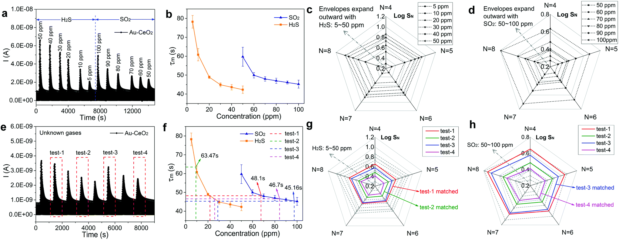 | ||
| Fig. 4 Quantitative identification of gas species. (a) The variation of sensor current for sensing H2S and SO2 with various concentrations. (b) The variation of τm of Au–CeO2 sensor for sensing H2S and SO2 with various concentrations. Radar charts for respectively detecting (c) H2S with a concentration ranging from 5 to 50 ppm, (d) SO2 with a concentration ranging from 50 to 100 ppm. (e) The variation of sensor current toward H2S and SO2 (test gas) with different concentrations, respectively. (f) The pre-judgements of the possible gases deduced by τm. The verifications of the pre-judgements by using radar charts of (g) H2S and (h) SO2. | ||
To verify the accuracy of the recognition library, we measure a series of sensor current curves when exposed to unknown gases as presented in Fig. 4e. Then, the identity of the unknown gas and its concentration were identified via a two-step judgment. Firstly, the current derivative curves were analyzed to acquire τm for pre-judgment. The acquired τm of the 4 groups are presented in Fig. S13† and Fig. 4f. For test-2, τm is 63.47 s and it is evident that the test gas is ∼9 ppm H2S. However, for test-1, τm is 48.1 s and therefore the test gas could either be ∼22 ppm H2S or ∼67 ppm SO2. Similarly, the gas in test-3 may be ∼28 ppm H2S or ∼97 ppm SO2 and the gas in test-4 may be ∼26 ppm H2S or ∼84 ppm SO2. In order to further identify the gas in test-1, test-3 and test-4, the radar charts (Fig. 4g and h) were analyzed. For example, the green envelope for test-2 is between 5 and 10 ppm H2S envelopes in Fig. 4g and does not match with the SO2 envelopes in Fig. 4h. Therefore, the gas in test-2 can be identified as ∼9 ppm H2S, fully consistent with the actual concentration. Similarly, the gases in test-1, test-3 and test-4 can be determined as ∼22 ppm H2S, ∼97 ppm SO2 and ∼84 ppm SO2, respectively.
Four additional test cases (i.e., test-5 through test-8) were also run to further confirm the accuracy of the gas recognition library. In Fig. S14a,† we demonstrate the detection of unknown gases from test-5 through test-8. First, to acquire the results of pre-judgment, τm calculated from current derivative curves have been analyzed in Fig. S14b.† For test-7, τm is ∼69.39 s and it follows that the test gas is ∼7 ppm H2S. However, for test-5, τm is ∼47.07 s and the test gas could be ∼25 ppm H2S or ∼80 ppm SO2. Similarly, the gas in test-6 may be ∼15 ppm H2S or ∼55 ppm SO2 and the gas in test-8 may be ∼26 ppm H2S or ∼91 ppm SO2. In order to further identify the gas in test-5, test-6 and test-8, radar charts (Fig. S14c and S14d†) were adopted. For example, the green envelope for test-7 is between the ∼5 and ∼10 ppm H2S envelopes in Fig. S14c† and does not match with the SO2 envelopes in Fig. S14d.† Therefore, the gas in test-7 can be identified as ∼7 ppm H2S consistent with the actual concentration. Similarly, the gases in test-5, test-6 and test-8 can be determined as ∼25 ppm H2S, ∼15 ppm H2S and ∼91 ppm SO2, respectively.
We have summarized the identification results of test-1 through test-8 in Table 2. It is evident that the gas recognition library can be used to discriminate between H2S and SO2 in a facile manner and the maximum recognition error is less than 16.67%. The main attractive feature of our method is that it does not rely on large-scale sensor arrays and complex algorithms.
| Test | Pre-judgement | Identification | True value | Error (%) |
|---|---|---|---|---|
| 1 | 22 ppm H2S | 22 ppm H2S | 19 ppm H2S | 15.79 |
| 67 ppm SO2 | ||||
| 2 | 9 ppm H2S | 9 ppm H2S | 9 ppm H2S | 0 |
| 3 | 28 ppm H2S | 97 ppm SO2 | 95 ppm SO2 | 2.11 |
| 97 ppm SO2 | ||||
| 4 | 26 ppm H2S | 84 ppm SO2 | 85 ppm SO2 | 1.17 |
| 84 ppm SO2 | ||||
| 5 | 25 ppm H2S | 25 ppm H2S | 25 ppm H2S | 0 |
| 80 ppm SO2 | ||||
| 6 | 15 ppm H2S | 15 ppm H2S | 13 ppm H2S | 15.38 |
| 55 ppm SO2 | ||||
| 7 | 7 ppm H2S | 7 ppm H2S | 6 ppm H2S | 16.67 |
| 8 | 26 ppm H2S | 91 ppm SO2 | 90 ppm SO2 | 1.11 |
| 91 ppm SO2 |
Furthermore, to prove the broad application of this two-step judgement process, in Fig. S15,† we have supplemented experiments for quantitatively detecting NO2 and NH3 with concentrations ranging from 20 ppm to 100 ppm, respectively. Similarly, the τm values of the Au–CeO2 sensor for NO2 and NH3 detection are respectively given in Fig. S16a,† it is obvious that there are obvious differences between these two curves. NO2 and NH3 radar chart are also constituted by a series of envelopes at various concentrations. To verify the accuracy of the recognition library, we have also measured a series of sensor current curves when exposed to test gases (test n1–n6), as presented in Fig. S16b and S16c.† All identification results are summarized in Table S5.† It is evident that the gas recognition library can be used to discriminate NO2 and NH3, and it also proved that the short period sinusoidal thermal modulation strategy has the ability to have broad applications for quantitatively detecting sorts of gases.
It is to be noted that in addition to the ability to distinguish between gas species our sensor exhibits high sensitivity. Under the short period sinusoidal heating voltage, the Au–CeO2 sensor exhibits an outstanding response value which nears ∼312.42% at a concentration of ∼50 ppm H2S (Fig. S9a†). The response value of the sensor device increases with increasing H2S concentrations from 5 to 50 ppm, and the fitting curve is also given in Fig. S9a,† where the determination coefficient (R2) is equal to 0.9848 suggesting that the sensor follows the Freundlich isotherm. The detection limit (DL) of the Au–CeO2 sensor is evaluated (refer to the ESI†) to be ∼1.059 ppm. Another noteworthy advantage of our sensor lies in its power consumption. The commercial FIGARO semiconductor gas sensors on the market consumes between 300 and 700 mW, and they were always beset by problems of cross-sensitivity of different gases. As indicated in Fig. S9b,† our sensor consumes only ∼144 mW of power, which greatly reduces the power dissipation. Furthermore, the ability to rapidly discriminate between and quantitatively identify the gas species is a unique strength of our sensor concept.
In Table 3, we have summarized the performances of our sensor and compared it with other H2S sensors reported in previous literature. It is evident that our sensor exhibits both high response value as well as fast response speed for sensing H2S at a relatively low temperature, and sinusoidal heating modulation of the sensor brings about much lower power consumption than commercial gas sensors. Most importantly, the introduced gas recognition library can be employed to quantitatively discriminate H2S from SO2, which is not possible with other sensor devices.
| Material | Conc. (ppm) | Temp. (°C) | S (%) | Res./rec. time | Identify from other gases | Power | Ref. |
|---|---|---|---|---|---|---|---|
| PPy/WO3 | 1 ppm | RT | 81% | 360 s/12600 s | No | — | 31 |
| SnO2 NWs/rGO | 50 ppm | RT | 33% | 2 s/292 s | No | — | 15 |
| SnO2 NFs/rGO | 5 ppm | 200 | 34% | ∼120 s/∼550 s | No | — | 32 |
| h-WO3/3D rGO | 10 ppm | 330 °C | 45% | 7 s/55 s | No | — | 33 |
| NiO/CuO | 100 ppm | 300 °C | 140% | 18 s/29 s | No | — | 34 |
| Figaro sensors | 100 ppm | 300 °C | — | — | No | ∼800 mW | 35 |
| Au/CeO2 | 50 ppm | ∼100 °C (max) | 312.42% | 60 s/198 s | Yes | ∼144 mW | This work |
Conclusions
To conclude, this paper introduced a two-step judgment process to rapidly discriminate and quantitatively identify H2S and SO2 by employing a single Au-doped CeO2 sensor. By applying a short period sinusoidal heating voltage to the Au–CeO2 sensor, we could rapidly obtain several sampling current curves at various sampling N values, and a gas recognition library for sensing H2S and SO2 was established by collecting the characteristic patterns. Validation tests were taken to verify the reliability, demonstrating that the recognition library based on the two-step judgment process had the ability to discriminate H2S and SO2 and sensitively detect their concentrations. The main attractive feature of our method is that it does not rely on large-scale sensor arrays and complex algorithms and is amenable for rapid (real-time) and low-power gas monitoring, which could find broad application in the area of chemical sensing.Experimental section
Materials
All reagents used in this experiment were analytically pure without further purification and purchased from Sinopharm Chemical Reagent Co., Ltd (Shanghai, China). The calibration gases (H2S and SO2) of ∼100 ppm that were purchased from Dalian Special Gases Co., Ltd were stored in a steel cylinder.Synthesis of CeO2 nanoparticles
The CeO2 NPs were synthesized using a facile one-step hydrothermal process. Under vigorous stirring, 0.484 g of Ce(NO3)3·6H2O and 0.496 g of polyvinylpyrrolidone were dissolved in a 100 mL dispersion containing deionized (DI) water and ethanol with a volume ratio of 1:3, followed by sonicating for five minutes. After that, 3 g urea was put into the obtained homogeneous suspension with magnetic stirring (600 rpm) for 30 min. Then, 80 mL of the above mixture was transferred into a 100 mL Teflon-lined autoclave and subjected to hydrothermal treatment at 180 °C for 18 h. After the autoclave cooled to room temperature, the obtained precipitates were collected by centrifugation at 5000 rpm for 5 min, and washed alternately with DI water and ethanol 2–3 times. Finally, the products were acquired by freeze drying for 24 h.
Functionalization of CeO2 nanoparticles with noble metals
10 mg of the prepared CeO2 NPs was dissolved in 20 mL DI water under sonication. Then, 105 μL of HAuCl4 (24 mM) was added to CeO2 dispersions, followed by putting 0.1 g of ascorbic acid into the homogeneous suspension with mild stirring and heating at 60 °C for 6 h. The obtained products were collected by centrifugation, rinsed repeatedly with water and ethanol for several times. Finally, the noble metal doped CeO2 NPs were freeze dried for 24 h.Characterization studies
The crystal phase of the pristine and functionalized CeO2 was analyzed with an X-ray diffractometer (Bruker D2 Phaser) using Cu Kα radiation (λ = 1.5418 Å) with a scanning range of 20°–90°. The surface morphology and nanostructure of the samples were examined by field emission scanning electron microscopy (Tescan MALA3 LMH). Morphologies and sizes of synthesized samples were studied using a high-resolution transmission electron microscope (HRTEM, JEM-2100F). Raman spectroscopy was taken in a back-scattering geometry using a single monochromator with a microscope (Reinishaw inVia) equipped with a CCD array detector (1024 × 256 pixels, cooled to −70 °C) and an edge filter. The samples were excited using a 514.5 nm Argon ion laser.Gas sensor fabrication
The dimensions of the ceramic substrate were 2 mm × 2 mm. Two gold test electrodes with a spacing of ∼150 μm were deposited in the front of the ceramic substrate. Furthermore, ruthenium oxides as heaters with a resistance of about 60 Ω were fabricated on the back side of ceramics via screen printing. An appropriate amount of deionized water was added to sensing material powders, and subsequently ground in an agate mortar. With a brush, the obtained slurry was uniformly coated on the gold test electrodes to form a gas sensing film. Then, the as-prepared sensor was dried at 60 °C for 24 h.Gas sensing experiments
The schematic illustration of the experimental instrument for gas sensing is shown in Fig. S1.† The sensing performances of sensors were tested in a stainless-steel chamber with a volume of 50 mL. Electrical feed-through, gas inlet and outlet were also designed in the chamber. Heating voltage was generated using a signal generator which had the ability to provide a DC or sinusoidal signal to drive the sensor after amplification by a power amplifier. The sensor current was measured using a picoammeter (Keithley 6485) at a DC voltage of ∼5 V. Dry air has been selected as the purging gas and the concentrations of the detected gas were adjusted by controlling the flow rate ratio between balance gas (air) and calibration gas, which could be achieved by utilizing mass-flow controllers (MFC). The ventilation time of target gas was set to around 100 s and the total gas flow rate was set to ∼100 sccm. It is noted that all gases we used were dry, thus there is no need to consider the effect of humidity after flushing the gas chamber with dry air for a period of time.Computational details
DFT+U calculations were performed using the Vienna ab initio simulation package (VASP).36,37 The electron–core interaction was described by the projector augmented wave (PAW) method. The electron exchange and correlation were treated with the generalized gradient approximation (GGA) using the Perdew–Burke–Ernzerhof (PBE) functional.38Ueff = 5.0 eV was used in all calculations to eliminate the error from strong self-interaction of the localized Ce 4f-orbital.39,40 The PBE-TS/HI method was adopted in all calculations to revise the deviation caused by van der Waals force.41 The CeO2 (111) surface was modeled using a 4 × 3 supercell with nine atomic layers and a vacuum layer of 15 Å to avoid the interaction between adjacent cells induced by the periodic boundary conditions.42,43 The bottom six layers of the model were fixed at bulk positions, while the remaining layers were fully relaxed during all the structure optimized calculations.44 All the calculations were carried out using the Brillouin zone sampled with a (2 × 2 × 1) gamma-centred mesh k-points grid,39 and a cutoff energy of 500 eV was adopted. For the structure optimization, the ionic positions were allowed to relax until the Hellman–Feynman forces were less than 0.02 eV Å−1.43 Electron charge analyses were performed by the Bader decomposition of the charge density.Conflicts of interest
There are no conflicts to declare.Acknowledgements
This work was supported by the National Key Basic Research Program of China (973 Program) (2015CB251001), the National Natural Science Foundation of China (No. 51877170), the Young Elite Scientists Sponsorship Program by the CAST, and the Fundamental Research Funds for the Central Universities. The calculations in this work were carried out on TianHe-2 at the LvLiang Cloud Computing Center. NK acknowledges the support from the John A. Clark and Edward T. Crossan Endowed Chair Professorship at the Rensselaer Polytechnic Institute, USA.Notes and references
- S. K. Pandey, K. Kim and K. Tang, TrAC, Trends Anal. Chem., 2012, 32, 87–99 CrossRef CAS.
- J. Chu, X. Wang, D. Wang, A. Yang, P. Lv, Y. Wu, M. Rong and L. Gao, Carbon, 2018, 135, 95–103 CrossRef CAS.
- D. Wang, X. Wang, A. Yang, J. Chu, P. Lv, Y. Liu and M. Rong, IEEE Electron Device Lett., 2018, 39, 292–295 CAS.
- A. Yang, D. Wang, X. Wang, J. Chu, P. Lv, Y. Liu and M. Rong, IEEE Electron Device Lett., 2017, 38, 963–966 CAS.
- D. Chen, J. Tang, X. Zhang, Y. Li and H. Liu, IEEE Sens. J., 2019, 19, 39–46 CAS.
- D. Chen, X. Zhang, J. Tang, H. Cui and Y. Li, Appl. Phys. A: Mater. Sci. Process., 2018, 124, 194 CrossRef.
- H. S. Wang, Y. G. Zhang, S. H. Wu, X. T. Lou, Z. G. Zhang and Y. K. Qin, Appl. Phys. B: Lasers Opt., 2010, 100, 637–641 CrossRef CAS.
- J. Petruci, A. Wilk, A. Cardoso and B. Mizaikoff, Anal. Chem., 2015, 87, 9605–9611 CrossRef CAS PubMed.
- J. P. Waclawek, R. Lewicki, H. Moser, M. Brandstetter, F. K. Tittel and B. Lendl, Appl. Phys. B: Lasers Opt., 2014, 117, 113–120 CrossRef CAS.
- W. Nakla, A. Wisitsora-at, A. Tuantranont, P. Singjai, S. Phanichphant and C. Liewhiran, Sens. Actuators, B, 2014, 203, 565–578 CrossRef CAS.
- Z. Wang, C. Zhao, T. Han, Y. Zhang, S. Liu, T. Fei, G. Lu and T. Zhang, Sens. Actuators, B, 2017, 242, 269–279 CrossRef CAS.
- D. Zhang, C. Jiang, P. Li and Y. E. Sun, ACS Appl. Mater. Interfaces, 2017, 9, 6462–6471 CrossRef CAS PubMed.
- A. Yang, D. Wang, X. Wang, D. Zhang, N. Koratkar and M. Rong, Nano Today, 2018, 20, 13–32 CrossRef CAS.
- Z. Jiang, J. Li, H. Aslan, Q. Li, Y. Li, M. Chen, Y. Huang, J. P. Froning, M. Otyepka, R. Zbořil, F. Besenbacher and M. Dong, J. Mater. Chem. A, 2014, 2, 6714–6717 RSC.
- Z. Song, Z. Wei, B. Wang, Z. Luo, S. Xu, W. Zhang, H. Yu, M. Li, Z. Huang, J. Zang, F. Yi and H. Liu, Chem. Mater., 2016, 28, 1205–1212 CrossRef CAS.
- H. Hu, X. Yang, X. Guo, K. Khaliji, S. R. Biswas, F. J. García De Abajo, T. Low, Z. Sun and Q. Dai, Nat. Commun., 2019, 10, 1131 CrossRef PubMed.
- D. Zhang, J. Liu, C. Jiang, A. Liu and B. Xia, Sens. Actuators, B, 2017, 240, 55–65 CrossRef CAS.
- S. De Vito, A. Castaldo, F. Loffredo, E. Massera, T. Polichetti, I. Nasti, P. Vacca, L. Quercia and G. Di Francia, Sens. Actuators, B, 2007, 124, 309–316 CrossRef CAS.
- J. Wu, K. Tao, Y. Guo, Z. Li, X. Wang, Z. Luo, S. Feng, C. Du, D. Chen, J. Miao and L. K. Norford, Adv. Sci., 2017, 4, 1600319 CrossRef PubMed.
- N. Illyaskutty, J. Knoblauch, M. Schwotzer and H. Kohler, Sens. Actuators, B, 2015, 217, 2–12 CrossRef CAS.
- L. Li, K. Yang, X. Bian, Q. Liu, Y. Yang and F. Ma, Sensors, 2019, 19, 3152 CrossRef PubMed.
- G. Zeng, C. Wu, Y. Chang, C. Zhou, B. Chen, M. Zhang, J. Li, X. Duan, Q. Yang and W. Pang, ACS Sens., 2019, 4, 1524–1533 CrossRef CAS PubMed.
- A. Larin, P. Womble and V. Dobrokhotov, Sensors, 2016, 16, 1373 CrossRef PubMed.
- V. Chaudhary and A. Kaur, RSC Adv., 2015, 5, 73535–73544 RSC.
- R. Kumar, D. K. Avasthi and A. Kaur, Sens. Actuators, B, 2017, 242, 461–468 CrossRef CAS.
- D. E. Motaung, G. H. Mhlongo, P. R. Makgwane, B. P. Dhonge, F. R. Cummings, H. C. Swart and S. S. Ray, Sens. Actuators, B, 2018, 254, 984–995 CrossRef CAS.
- H. Xia, Y. Wang, F. Kong, S. Wang, B. Zhu, X. Guo, J. Zhang, Y. Wang and S. Wu, Sens. Actuators, B, 2008, 134, 133–139 CrossRef CAS.
- B. M. Reddy, A. Khan, P. Lakshmanan, M. Aouine, S. Loridant and J. Volta, J. Phys. Chem. B, 2005, 109, 3355–3363 CrossRef CAS PubMed.
- D. Zhang, Y. E. Sun, P. Li and Y. Zhang, ACS Appl. Mater. Interfaces, 2016, 8, 14142–14149 CrossRef CAS PubMed.
- H. Zhang, J. Feng, T. Fei, S. Liu and T. Zhang, Sens. Actuators, B, 2014, 190, 472–478 CrossRef CAS.
- P. Su and Y. Peng, Sens. Actuators, B, 2014, 193, 637–643 CrossRef CAS.
- S. Choi, B. Jang, S. Lee, B. K. Min, A. Rothschild and I. Kim, ACS Appl. Mater. Interfaces, 2014, 6, 2588–2597 CrossRef CAS PubMed.
- J. Shi, Z. Cheng, L. Gao, Y. Zhang, J. Xu and H. Zhao, Sens. Actuators, B, 2016, 230, 736–745 CrossRef CAS.
- Y. Wang, F. Qu, J. Liu, Y. Wang, J. Zhou and S. Ruan, Sens. Actuators, B, 2015, 209, 515–523 CrossRef CAS.
- K. A. Ngo, P. Lauque and K. Aguir, Sens. Mater., 2006, 18, 251–260 CAS.
- Z. Yang, T. K. Woo and K. Hermansson, Surf. Sci., 2006, 600, 4953–4960 CrossRef CAS.
- H. Cui, X. Zhang, G. Zhang and J. Tang, Appl. Surf. Sci., 2019, 470, 1035–1042 CrossRef CAS.
- H. Jia, B. Ren, M. Li, X. Liu, J. Wu and X. Tan, Solid State Commun., 2018, 277, 45–49 CrossRef CAS.
- M. D. Krcha and M. J. Janik, Surf. Sci., 2015, 640, 119–126 CrossRef CAS.
- M. Nolan, S. Grigoleit, D. C. Sayle, S. C. Parker and G. W. Watson, Surf. Sci., 2005, 576, 217–229 CrossRef CAS.
- D. Wang, X. Wang, A. Yang, P. Lv, J. Chu, Y. Liu, M. Rong and C. Wang, Mater. Chem. Phys., 2018, 212, 453–460 CrossRef CAS.
- J. Wang and X. Gong, Appl. Surf. Sci., 2018, 428, 377–384 CrossRef CAS.
- J. J. Carey and M. Nolan, Appl. Catal., B, 2016, 197, 324–336 CrossRef CAS.
- B. Milberg, A. Juan and B. Irigoyen, Appl. Surf. Sci., 2017, 401, 206–217 CrossRef CAS.
Footnotes |
| † Electronic supplementary information (ESI) available. See DOI: 10.1039/c9nr05863j |
| ‡ These authors contributed equally. |
| This journal is © The Royal Society of Chemistry 2020 |