
 Open Access Article
 This Open Access Article is licensed under a Creative Commons Attribution-Non Commercial 3.0 Unported Licence
Exploration of mechanical, thermal conductivity and electromechanical properties of graphene nanoribbon springs†
Brahmanandam
Javvaji
 a,
Bohayra
Mortazavi
a,
Timon
Rabczuk
bc and
Xiaoying
Zhuang
*de
a,
Bohayra
Mortazavi
a,
Timon
Rabczuk
bc and
Xiaoying
Zhuang
*de
aChair of Computational Science and Simulation Technology, Department of Mathematics and Physics, Leibniz Universität Hannover, Applestr. 11, 30167 Hannover, Germany
bInstitute of Structural Mechanics, Bauhaus University Weimar, Marienstrasse 15, 99423 Weimar, Germany
cCollege of Civil Engineering, Department of Geotechnical Engineering, Tongji University, Shanghai, China
dDivision of Computational Mechanics, Ton Duc Thang University, Ho Chi Minh City, Vietnam
eFaculty of Civil Engineering, Ton Duc Thang University, Ho Chi Minh City, Vietnam. E-mail: xiaoying.zhuang@tdtu.edu.vn
First published on 28th May 2020
Abstract
Recent experimental advances [Liu et al., npj 2D Mater. Appl., 2019, 3, 23] propose the design of graphene nanoribbon springs (GNRSs) to substantially enhance the stretchability of pristine graphene. A GNRS is a periodic undulating graphene nanoribbon, where undulations are of sinus or half-circle or horseshoe shapes. Besides this, the GNRS geometry depends on design parameters, like the pitch's length and amplitude, thickness and joining angle. Because of the fact that parametric influence on the resulting physical properties is expensive and complicated to examine experimentally, we explore the mechanical, thermal and electromechanical properties of GNRSs using molecular dynamics simulations. Our results demonstrate that the horseshoe shape design GNRS (GNRH) can distinctly outperform the graphene kirigami design concerning the stretchability. The thermal conductivity of GNRSs was also examined by developing a multiscale modeling, which suggests that the thermal transport along these nanostructures can be effectively tuned. We found that however, the tensile stretching of the GNRS and GNRH does not yield any piezoelectric polarization. The bending induced hybridization change results in a flexoelectric polarization, where the corresponding flexoelectric coefficient is 25% higher than that of graphene. Our results provide a comprehensive vision of the critical physical properties of GNRSs and may help to employ the outstanding physics of graphene to design novel stretchable nanodevices.
1 Introduction
During the last decade, graphene1–3 the two-dimensional (2D) form of sp2 carbon atoms has attracted astonishing attention of scientific and industrial communities, stemming from its extraordinarily high mechanical4 and thermal5 conductivity properties along with exceptional electronic and optical characteristics. In particular, graphene can exhibit a remarkably high Young's modulus and tensile strength of 1000 GPa and 130 GPa (ref. 4) respectively, along with a superior thermal conductivity of around 4000 W mK−1 (ref. 6) that outperforms diamond and other conventional materials. The exceptional physical and chemical properties of graphene, promoted the experimental and theoretical endeavours to fabricate novel graphene's 2D counterparts, and subsequently explore their intrinsic properties and application prospects. As a result of scientific accomplishments, the 2D materials family is commonly considered as the most vibrant class of materials, in which new members are continuously introduced, either theoretically predicted or experimentally fabricated. It is worthy reminding that despite the outstanding properties of pristine graphene, it is not an ideal material and naturally shows a few drawbacks, such as the lack of an electronic band-gap and brittle failure mechanism.4,7 In addition, the ultra-high thermal conductivity of graphene also prohibits its application for thermoelectric energy generation.Nonetheless, it has also been practically proven that graphene can show largely/finely tunable electronic, mechanical, thermal, optical and electromechanical properties, with accurately controlled mechanical straining,8–13 defect engineering14–17 or chemical doping.18–22 We remind that for many centuries, springs have been playing pivotal roles in the design and fabrication of various kinds of devices. The importance of springs originates from the fact that while the mechanical properties of a material is considered as its inherent properties and thus invariable, when it is shaped in the form of springs the subsequent structures can show superior stretchability and diverse mechanical responses. In particular, the design of spring like structures has been known as one of the most effective approaches to achieve highly stretchable and flexible moving components.
For the employment of graphene in flexible nanoelectronics, its ductile and highly rigid mechanical properties are undesirable. Therefore, engineering of the graphene design in order to improve its stretchability is a critical issue.23–27 To address this challenge, in a most recent exciting experimental advance by Liu et al.28 the old idea of spring design has been applied in the case of graphene to enhance its stretchability and flexibility via a nanowire lithography technology. This experimental study consequently raises questions concerning how the design of graphene springs can be improved to reach higher degrees of stretchability. In addition, the electronic and heat transport properties of these novel nanostructures should also be examined, in order to provide comprehensive visions for the design of nanodevices. As a common challenge in an electronic apparatus, the thermal conductivity of employed components should be high to effectively dissipate excessive heat. On the other hand, low thermal conductivity is a key requirement for the enhancement of the efficiency of thermoelectric energy conversion. As a common barrier, it is well known that the evaluation of the mechanical and transport properties of graphene springs by experimental tests is not only complicated but also time consuming and expensive as well. This study therefore aims to investigate the mechanical response and heat conduction properties of graphene springs via conducting extensive classical molecular dynamics simulations. Since graphene is the first member of 2D materials, commonly the experimental and theoretical methodologies that are applied for graphene can be extended to the other members of the 2D materials family. We are thus hopeful that the results obtained by this study may serve as valuable guides for future theoretical and experimental studies on the design of 2D spring material like structures.
2 Methods
We conducted classical molecular dynamics (MD) simulations to evaluate the mechanical properties and thermal conductivity of graphene springs, using the Large scale Atomic/Molecular Massively Parallel Simulator package.29 To this aim, we used the optimized Tersoff potential parameter set proposed by Lindsay and Broido30 for introducing the atomic interaction between carbon atoms. This version of Tersoff potential is not only highly computationally efficient, but also can yield accurate results for the mechanical and thermal properties of graphene. We analysed the mechanical response by conducting the uniaxial tensile simulations at room temperatures. For the evaluation of mechanical properties, we modified the cutoff of Tersoff potential from 0.18 nm to 0.20 nm to remove an unphysical stress pattern and moreover accurately reproduce the experimental results for the tensile strength of pristine graphene.31 In this case, the time increment of MD simulations was set at 0.25 fs. Before applying the loading conditions, all the structures were equilibrated using the Nosé–Hoover thermostat method. For the loading conditions, a constant engineering strain rate of 1 × 10⁸ s−1 was applied, by increasing the periodic size of the simulation box along the loading direction in every time step. Virial stresses at every step were recorded and averaged over every 20 ps interval to report the stress–strain relations. To evaluate the thermal conductivity, we used the equilibrium molecular dynamics (EMD) method. The time increment of EMD simulations was set at 0.25 fs. In the EMD method, the heat flux vector was calculated via: | (1) |
 | (2) |
3 Results
Fig. 1(a) and (b) show the atomic unit-cell representation for the graphene nanoribbon (GNR) in the sinus shape and horseshoe shape, respectively. The sinus shape GNR (GNRS) was obtained from cutting the infinite graphene sheet using two sine curves that are parallel to each other. The parameters defining the sine curve are the pitch length (sp) and amplitude (sa). The locus of each point normal with a constant length (st) creates a parallel sine curve. The variable st defines the thickness of the GNRS. The choice of sp and sa is arbitrary. However, st should be less than the radius of the curvature of the sine curve to avoid producing bigger arcs that cover the crests and troughs (cusps) of the sine curve. Using these variables for the GNRS, we define a sinus shaped region on a pristine graphene sheet and removed atoms in the other regions, which creates an initial atomic configuration for the GNRS. The volume of the GNRS is defined as the area under the parallel sine curve multiplied by the thickness of the pristine graphene sheet 3.3 Å.32 | ||
| Fig. 1 Unit cell representation and definition of various structural parameters for the (a) sinus shape and (b) horseshoe shape graphene nanosprings. | ||
The horseshoe shape design GNR (GNRH) was composed by connecting two circular arcs of the inner radius (hr) with the intersecting angle (hθ). When hθ = 0°, the GNRH looks like a series of connected semi-circles and for hθ > 0° and hθ ≤ 45°, the horseshoe design is obtained. For hθ more than 45°, the semi-circles merge with each other, which is not desirable. These parameters define the shape of a single horseshoe curve. Another curve with radius hr + ht creates a parallel curve, where ht defines the thickness of the GNRH. We constructed the horseshoe-shaped region on a pristine graphene sheet and removed atoms in the other regions, which creates an initial atomic configuration for the GNRH system. After the initial preparation of the spring structures, we removed the carbon atoms bonded with a single carbon atom along the lateral edges since these atoms can lead to instability in simulations. It is worth noting that the carbon atoms belonging to the curved edges of the GNRS and GNRH system are not terminated with hydrogen atoms.
With the defined geometrical parameters and initial atomic configurations for the GNRS and GNRH, we consider the following parameter sets for estimating the mechanical and thermal properties. Parameter setsp–st–sa: the starting value for sp is 9 nm (where the size effects are absent in pristine graphene13), and sa is 2.5 nm, where at least 10 carbon rings accompany in the lateral direction. The minimum possible value of st is 1.6 nm for this combination of sp and sa for having a reasonable thickness for these spring systems. Further, we increase the values of sp, st and sa by integral multiples from 1 to 5. Parameterhθ: we consider hθ to be 0°, 15°, 30° and 45° by keeping hr at 2.5 nm and ht as 1.6 nm. Using this choice of parameters, we explore the effect of hθ on mechanical and thermal properties. Parameterhr–ht: in this set, hr and ht parameters are scaled by integral multiples from 1 to 5 starting from 2.5 and 1.6 nm at fixed hθ. We fix the value of hθ from the previous parameter set, which has shown exceptional mechanical properties. The spring structures from the different parameter sets are made by cutting from graphene sheets oriented along the zigzag direction. Our comparative results discussed in the ESI† document however confirm that the orientation of the original graphene sheet shows negligible effects on the estimated properties.
3.1 Mechanical properties
Fig. 2(a) shows the stress–strain curves for the parameter set sp – st – sa. Under stretching of the GNRS system, the stress values remain low up to a strain of 0.3. This behavior is in contrast to that of pristine graphene. The given deformation stretches the bond lengths in pristine graphene and increases the stress levels. In GNRS systems, the given deformation deflects the atomic system instead of stretching the bonds, which is similar to the earlier observations for graphene kirigami.33 Further, a recent study on nonlinear vibrations for a helical graphene nanoribbon shows a transformation of a softening type to a hardening type response between the amplitude and frequency variation during the increase in mechanical loading.34 In the GNRS, the initial plateau in the stress–strain curve up to a strain of 0.3 corresponds to the soft nonlinearity. Because of the transformation from softening to hardening type natural vibrations, the GNRS system starts stretching due to the increased loading. Fig. 3(a) shows the initial (strain is 0) atomic configuration for the 18 – 3.2 – 5 GNRS. A visual molecular dynamics package35 has been used to generate the atomic snapshots. At a strain of 0.18, because of the deflections, a higher number of crests and troughs are observed in Fig. 3(b). Further straining to 0.30 deflects the GNRS without increasing the peaks (Fig. 3(c)). For a strain less than 0.30, there is no significant increase in the stress distributions. When strain is more than 0.30, there is an increase in stress due to the bond stretching. Fig. 3(d) shows the locations of stress concentrations (near peaks) in the atomic configurations. The atomic configuration in Fig. 3(e) shows the multiple bond failures at a strain of 0.54. The failure process for other members in this parameter set is similar to the configuration of the 18 – 3.2 – 5 GNRS. However, there are differences in the tensile strength (TS) and onsite failure/rupture strain (RS) values due to the changes in the geometrical parameters. We use the arc length as the variable to discuss the parametric dependence of RS and TS on sp, st and sa. Fig. 2(d) shows that RS is nearly converged to 0.45 for arc lengths larger than 170 nm. However, TS has a very large variation with arc length, from 33 to 7 GPa, which is due to the increase of parameter st in the GNRS design. As st increases, the interaction between stress centers near crest and troughs of the GNRS decreases, which decreases the total system stress. Further increase in the size parameters will converge to a constant value. Finally, for GNRS systems, the stress concentratations near the peak portions lead to global failure by breaking the bonds in the carbon rings. The RS for the experimentally manufactured GNRS is about 0.35 for a system with the thickness 50 nm.28 This observation is in close agreement with the converged RS value of 0.43 for the spring design, which shows that our simulation predictions are accurate enough to explore the theoretical understanding of these novel designs. | ||
| Fig. 2 Stress–strain curves for (a) parameter set sp – st – sa in the GNRS, and (b) hθ and hr – ht for the GNRH. (c) Standard deviation of the z− coordinates for the selected GNRS and GNRH systems. (d) Variation of the rupture strain and tensile strength (TS) for GNRS and GNRH systems with arc length. Solid lines indicate RS and dashed lines correspond to TS. | ||
 | ||
| Fig. 3 Tensile deformed atomic configurations for (a–e) 18 – 3.2 – 5 GNRS and (f–j) 5 – 3.2 – 45° GNRH. The strain levels for the atomic snapshots are as follows: (a and f) 0.0, (b) 0.18, (c) 0.30, (d) 0.42, (e) 0.54, (g) 1.42, (h) 2.0, (i) 2.17 and (j) 2.23. The color bar indicates the stress values. | ||
Fig. 2(b) shows the stress–strain response for parameter set hθ, where hr and ht values are 2.5 and 1.6 nm, respectively. When hθ = 0°, there is no stress rise up to a strain of 0.3. For the strain range 0.3 to 0.6, the deformation in atomic configuration raises the system stress followed by a failure. The strain range for the non-zero portion of the stress–strain curve shifts between 0.5 and 1.0 when hθ is 15°. For hθ equal to 30°, the non-zero portion of the stress–strain curve span the strain range of 0.94 to 1.5. For the 45° GNRH, this strain range increased to 2.4. Fig. 3(f)–(j) show the atomic configurations for a GNRH with a 45° connecting angle. The closeness between semi-circular segments in the GNRH develops strong repulsive interactions compared to those in the GNRS. Such repulsion largely deflects the atomic system. Further, mechanical stretching reduces atomic deflections by maintaining the stress levels via transforming the smooth circular GNRH segments to sharp peaks. Fig. 3(g) shows the atomic configuration with several peaks for the GNRH. For a strain greater than 1.5, Fig. 2(b) shows a linear stress–strain response due to the bond stretching. At a strain of 2, the GNRH system looks like a combination of thread and knots, as seen in Fig. 3(h), where stress concentrates near the thread portions. Further increase in the strain in the GNRH leads to bond failure. Fig. 3(i) and (j) at strain levels of 2.17 and 2.23 show the complete failure of the GNRH.
Interestingly, the GNRH with various hθ values maintained the stress levels when increasing the strain range. We consider varying the width parameter ht in the GNRH by keeping the other parameters constant to check its influence on the mechanical properties. The range of ht is limited by the choice of the other two parameters. For example, consider that hr is equal to 5 nm and hθ is 45°. The maximum available value of ht is 4 nm. When ht is greater than 4 nm, the two circular cross-sections of the GNRH unit cell overlap with each other, which is not desirable. We consider ht values to be 1.6, 2.4 and 3.2 and 4 nm and the corresponding RS values are 2.64, 2.44, 2.17 and 1.9, respectively. TS values are noted as 53.83, 38.06, 24.81 and 17.49 GPa (see the ESI†). When varying hθ, the RS increased with a very low effect on TS (see circle markers with dotted and solid lines in Fig. 2(d)). However, variation of ht has an effect on both RS and TS in the GNRH. The increase in thickness increases the separation between the stress centers and decreases the TS, which leads to early failure and decrease in RS. This finding implies that the change of ht strongly influences both RS and TS of the GNRHs. The observations concerning the width effect on the mechanical response are in close agreement with those of an earlier report based on MD simulations.36
When compared to the GNRS, the GNRH shows higher stress levels (dotted lines in Fig. 2(d)). From the structural point of view, the GNRH differs from GNRS in two factors, one is the smoothness of undulations and the second is the closeness between the undulations. The smoothness of circular arcs in the GNRH makes the stress distribute across all the boundary atoms. The increased number of atoms with higher per atom stress values increases the total stress in the atomic system. In the case of the GNRS, the lower number of atoms with higher per atom stress near the peaks of the sine curve makes the total stress lower. From Fig. 2(d), it can be seen that the TS values for the 2.5 – 1.6 – 0° GNRH and 9 – 1.6 – 2.5 GNRS are 39.72 and 31.93 GPa, respectively, which represents that the smoothness factor accommodates more number of atoms with high stress levels in the horseshoe shape design. The closeness between the undulations increases the deflections in the atomic system, which helps to avoid the bond stretching and stress rise. These deflections in GNRS and GNRH systems are measured using the standard deviation of the z-coordinates (![[Z with combining macron]](https://www.rsc.org/images/entities/i_char_005a_0304.gif) ),37 which is defined as
),37 which is defined as 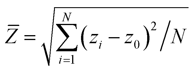 , where zi is the z-coordinate of the ith atom and z0 is the averaged z-coordinate over N atoms. Fig. 2(c) shows the computed with respect to strain for the selected GNRS (9 – 1.6 – 2.5) and GNRH (parameter set hθ) systems. initially increases with strain, which represents that the energy of given mechanical strain is used to increase the deflections in both GNRH and GNRS systems. After reaching a maximum deflection, the given tensile loading starts stretching the atomic system and decreasing the deflections which decrease . However, the magnitude of for the 0° GNRH configuration is high compared to that of the 9 – 1.6 – 2.5 GNRS, which supports that the repulsive interactions in the GNRH are heavier compared to those in the GNRS. increases with an increase in parameter hθ. is highest for the 45° GNRH.
The very strong repulsions exist between the semi-circular rings due to the minimum spacing. The very high deflections and smoothness of circular cross-sections help to avoid the stress concentrations in the GNRH, which helps to enhance the mechanical properties. As a result, a very high value of RS is noted for the GNRH. With the increasing system size (arc length of the GNRH), RS tends to converge to a value of 2, which is about 17% higher than that of the graphene kirigami design,38,39 keeping the stress-levels identical.
3.2 Thermal properties
We next study the thermal transport through the GNRS and GNRH systems. Fig. 4 shows the EMD results of the effective thermal conductivity of the GNRS for the few studied parameter sets, as a function of correlation time. In this case, we normalized the effective conductivity with respect to that of the pristine graphene to better illustrate the suppression rate. As is clear, for the samples with lower thermal conductivity the convergence occurs at lower correlation times. For the 9 – 1.6 – 2.5 GNRS, κ is about 0.0175 times the thermal conductivity of pristine graphene κ0 (from Fig. 4(a)). We employed a square sheet of pristine graphene with a 16 nm side length to estimate κ0. The estimated value of κ0 is 1000 ± 100 W (mK−1), which is an average over 8 independent simulations. This value is in close agreement with that of earlier reports using the EMD method.40 Note that due to the implementation of the inaccurate heat-flux formula for many-body interactions in the LAMMPS tool, the EMD method significantly underestimates the thermal conductivity of graphene.41 The suppressed thermal transport along the GNRS is due to the phonon-boundary scattering in these systems, which is in accordance with the previous reports concerning graphene kirigami.33 Also, there occurs very strong conversion for the phonon mode polarization from out-of-plane to in-plane and the opposite phase for the left and right parts of the unit cell.42,43 The loss in thermal energy transport is due to the conversion of phonon modes through the scattering with localized phonon modes near the edges. As a result the transport of heat flux is low and reduces the thermal conductivity. When st increases, the ratio of atoms on the boundaries to the total number of atoms decreases, which results in the lower phonon-boundary scattering rate and subsequently facilitates the heat transport.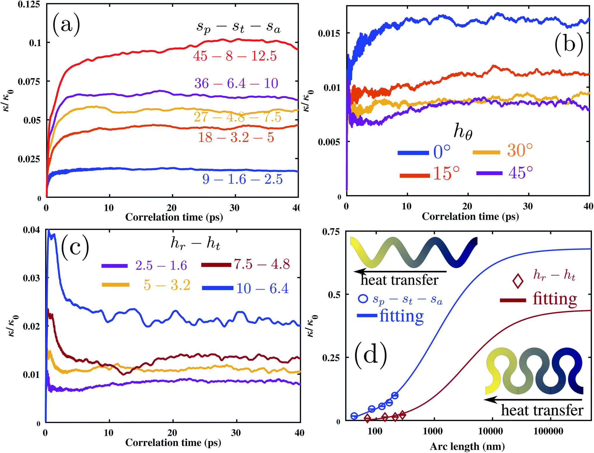 | ||
| Fig. 4 Room temperature thermal conductivity for (a) parameter set sp – st – sa in the GNRS, (b) hθ and (c) hr – ht for the GNRH as a function of correlation time. (d) Thermal conductivity of the graphene nanosprings at room temperature as a function of arc lengths. The insets in (d) illustrate the finite element modeling results for temperature distribution of the GNRS and GNRH in the diffusive regime. | ||
As proposed in previous work,33 we use a microscale continuum model of the graphene springs to evaluate the effective thermal conductivity. This evaluation was carried out within the diffusion range, in which the phonon-boundary scattering vanishes. To this aim, a system is modeled by the finite element (FE) approach to establish connections between the effective thermal conductivity and nanoribbon's arc length. We apply inward and outward heat-fluxes on the two opposite sides of the GNRS as the boundary conditions. Using the measured temperature gradient along the heat transfer direction, the effective thermal conductivity was computed from Fourier's law. We then used a first order rational curve fitting to extrapolate the atomistic results (circular markers in Fig. 4(d) that correspond to the averaged κ/κ0 over several samples of sp – st – sa and the standard deviation among them) dominated by the phonon-boundary scattering to the diffusive transport by the FE simulations. As shown in Fig. 4(d), this approach could provide a very accurate estimation of thermal transport at different arc lengths, and reveals that the phonon-boundary scattering starts to vanish at large arc lengths.
For the GNRH systems κ/κ0 with varying hθ is shown in Fig. 4(b). κ/κ0 for the 2.5 – 1.6 – 0° GNRH is about 0.0169, which is nearly the same as for the 9 – 1.6 – 2.5 GNRS. The constant thickness and similar scattering effects in these two spring systems produce the nearly equal thermal conductivity. Keeping thickness constant and increasing the joining angle hθ to 15°, κ/κ0 decreased from 0.0169 to 0.0111. As hθ increases, there is an increase in the radius of curvature of the junction region that connects the two semi-circular segments. The phonon transport through this increased curvature experiences significant scattering, which reduces the heat transfer and κ. The thermal conductivity for hθ 30° and 45° is nearly the same.
We examine the thermal conductivity for the GNRH samples used in estimating the effect of width on mechanical properties in Section 3.1. The effective thermal conductivity for 2.5 – 1.6 – 45° and 5 – 1.6 – 45° are 0.0084 and 0.0055. This represents that increase in hr increases the radius of curvature and produces more edge localized phonon modes. These modes do not contribute to thermal transport; as a result the thermal conductivity decreases for the 5 – 1.6 – 45° GNRH system (see the ESI†). However, the increase in ht increases the number of phonon modes in the GNRH keeping the density of edge localized modes the same. This reduces the edge scattering and increases the phonon transport, thus increasing κ.44Fig. 4(c) shows κ for increasing values of hr and ht keeping the joining angle hθ as 45°. As the GNRS radius and thickness increase, the available region for heat transport increases, which helps to lower the scattering and increase κ/κ0 from 0.0084 to 0.0216. This increase of κ is small compared to that of the GNRS systems due to the large curvature induced scattering. We repeat the FE modeling for the GNRH with hθ as 45° similar to the GNRS. The fitting between atomistic results and FE modeling is very good. However, GNRH fitting is converged at significantly larger cut lengths compared to GNRS fitting. This proves that curvature induced scattering reduces κ in the GNRH.
3.3 Electromechanical properties
The nanoscale electromechanical properties (piezoelectricity and flexoelectricity) have been gaining intense attention due to their ability to sustain large deformations. This feature adds many different applications in the energy conversion process. These properties are limited in pristine graphene due to the crystallographic symmetry. The structural and chemical modifications break the symmetry and induce polarization under mechanical deformations.17,45–50 The bending deformation of pristine graphene induces a polarization due to the change of the hybridization state of the carbon atom, known as pyramidalization.48,51,52 In GNRS and GNRH systems, cut patterns cancel the symmetry and show promise for electromechanical coupling. In this section, we subject the GNRS and GNRH system to both tensile and bending deformations to obtain the respective polarization variations.To calculate the polarization in the atomic system, we utilize the charge–dipole (CD) model along with the short-range bonded interactions (Tersoff potential). According to the CD model, each atom i is associated with charge qi and dipole moment pi.53,54 The mathematical CD formulation involves the various contributions from charge–charge, charge–dipole and dipole–dipole interactions to the total system short-range interaction energy. The minimization of the energy function gives the numerical values of qi and pi. The complete details about the CD model and estimation of charges and dipole moments can be found in ref. 17 and 52 and references therein.
For applying deformation, we have added left and right rectangular regions to the GNRS and GNRH systems by discarding the periodic boundary condition used in Section 2. These regions have equal st or ht to those of the spring systems with 1 nm length along the spring longitudinal direction. The left and right regions help to hold the given displacement, particularly during the bending test, and relax the remaining system. We define a load cycle by prescribing the displacement of atoms to left and right regions for a 1 ps time period, followed by a relaxation for a 2 ps time period. Because of the nonperiodic boundaries, we perform simulations at different repetitions of sinus and horseshoe shapes in spring systems. These simulations help us to study the size effect on electromechanical properties. For every load cycle, we note the evolution of the atomic configuration, and the corresponding charge and dipole moments. The total polarization of the atomic system is the sum of all atomic dipole moments divided by the volume of the atomic system.
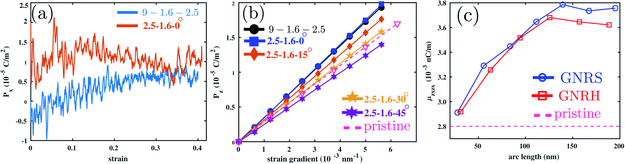
For tensile deformation, we apply a displacement in the longitudinal direction ux = ![[small epsi, Greek, dot above]](https://www.rsc.org/images/entities/i_char_e0a1.gif) tloadl0 to the atomic system, where is the strain rate, equal to 1 × 10⁸ s−1 as used in Section 2, tload is the loading time (1 ps) and l0 is the initial length of the atomic system in the longitudinal direction. The load cycles continued to reach a strain εxx of 0.4 for 9 – 1.6 – 2.5 and 2.5 – 1.6 – 0° systems. The strain limit 0.4 corresponds to the linear rise in the stress–strain response for these systems as shown in Fig. 2(a). At each load cycle, the polarization is measured and the variation with strain is plotted in Fig. 5(a). The variation in polarization with strain is nearly negligible for both GNRS and GNRH systems. The coefficient of variation for the polarization response is nearly equal to 1 for both the GNRS and GNRH, similar to non-piezoelectric pristine graphene.17 The cancellation of polarization at the sinus and horseshoe cut patterns makes these systems non-piezoelectric materials.
tloadl0 to the atomic system, where is the strain rate, equal to 1 × 10⁸ s−1 as used in Section 2, tload is the loading time (1 ps) and l0 is the initial length of the atomic system in the longitudinal direction. The load cycles continued to reach a strain εxx of 0.4 for 9 – 1.6 – 2.5 and 2.5 – 1.6 – 0° systems. The strain limit 0.4 corresponds to the linear rise in the stress–strain response for these systems as shown in Fig. 2(a). At each load cycle, the polarization is measured and the variation with strain is plotted in Fig. 5(a). The variation in polarization with strain is nearly negligible for both GNRS and GNRH systems. The coefficient of variation for the polarization response is nearly equal to 1 for both the GNRS and GNRH, similar to non-piezoelectric pristine graphene.17 The cancellation of polarization at the sinus and horseshoe cut patterns makes these systems non-piezoelectric materials.
 | ||
| Fig. 5 (a) Variation of polarization Px with tensile strain. (b) Bending induced polarization Pz response with respect to the strain gradient. (c) Dependence of the flexoelectric coefficient μzxzx on the arc length of GNRS and GNRH systems. Legends indicate the respective atomic configurations used. | ||
For bending deformation, we supply the following out-of-plane displacement field to the atomic system
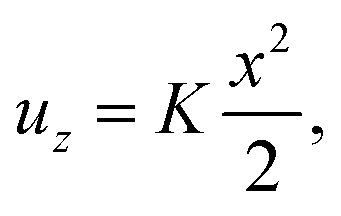 | (3) |
 | (4) |
 | (5) |
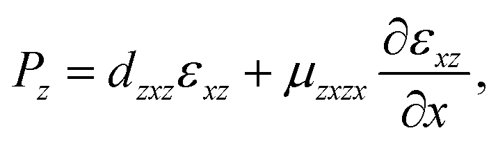
| Pz = μzxzxKeff. | (6) |
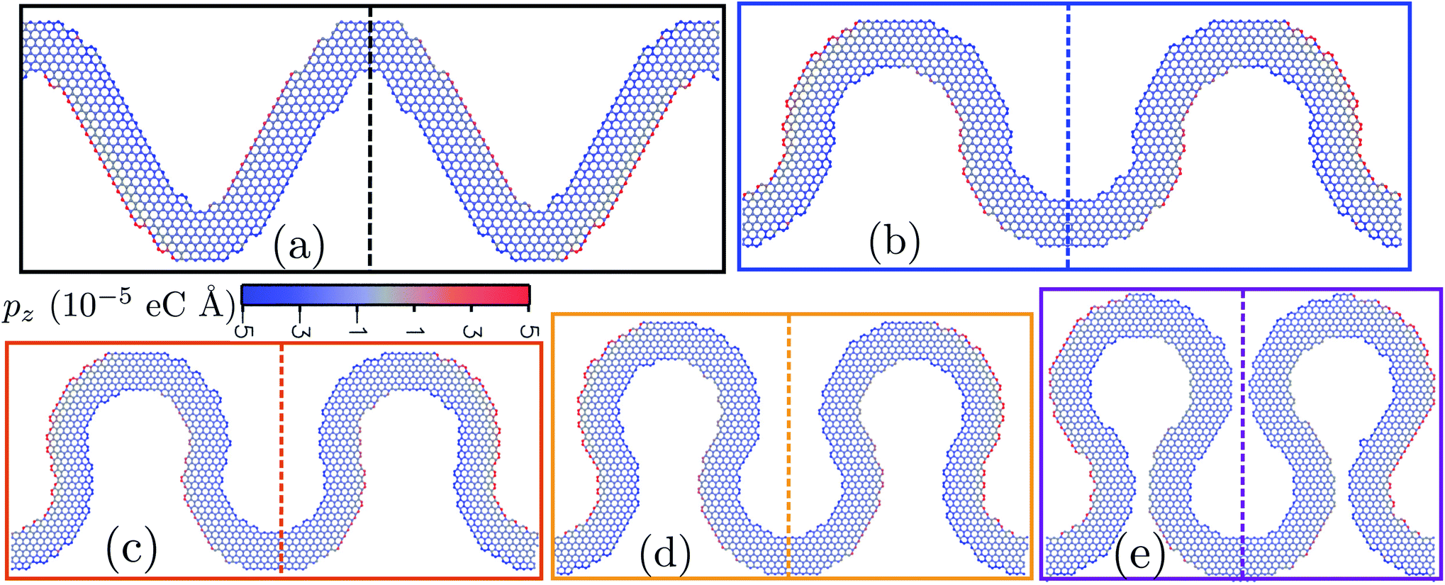 | ||
| Fig. 6 Atomic configurations colored with dipole moment pz for a strain gradient of 0.006 nm−1. (a) 9 – 1.6 – 2.5 GNRS design. GNRH design with the inner radius 2.5 nm, thickness 1.6 nm and connecting angle hθ at (b) 0°, (c) 15°, (d) 30° and (e) 45°. The dashed line indicates the middle portion of the atomic system. | ||
From Fig. 5(b), it can be seen that the slope of the polarization to strain gradient curve decreases with the increase of hθ in GNRH systems. The ratio of the change in the pyramidalization angles in GNRH and pristine graphene decreases to 1.27, 1.14 and 1.05 and 0.85 with hθ at 0°, 15°, 30° and 45°, respectively. The decrease in θσπ decreases the dipole moment distribution, as seen from Fig. 6(c) to (d), which decreases the flexoelectric coefficient. For hθ = 45°, the atoms on the lateral boundaries near the central line do not have dipole moments. The strong repulsions between these edges cancel the effect of pyramidalization, which decreases the flexoelectric coefficient.
In order to check the dependence of ht on the polarization, we consider 2.5 – 2.4 – 0° and 2.5 – 3.2 – 0° GNRH configurations. For these configurations, the polarization variation and flexoelectric coefficient are nearly equal to those of the 2.5 – 1.6 – 0° GNRH. The increase in thickness does not affect the induced polarization and flexoelectric coefficient (see the ESI†). The increased thickness was unable to change the pyramidalization angle further, which makes the polarization comparable with that of smaller thickness systems.
Further, the result of the flexoelectric coefficient with length variation is given in Fig. 5(c) for GNRS and GNRH (hθ = 0°). This result represents that there is a boundary effect when the arc length is less than 100 nm. For systems with an arc length about 30 nm, the local electric field is strongly affected by the left and right region of atoms. Here the imposed boundary condition constrains the natural motion of the interior atoms, which restricts the process of pyramidalization and controls the dipole moment. When increasing the arc length this effect slowly nullifies and the atomic configuration deforms to generate the dipole moments. For systems with lengths higher than 100 nm, the boundary effect is completely negligible and the flexoelectric coefficients turn into a stable value. Finally, the flexoelectric coefficient of the GNRS and GNRH-0° system is 0.25 times higher than that of pristine graphene.
4 Conclusion
Motivated by a latest experimental study, we performed extensive classical molecular dynamics simulations to explore the mechanical, thermal conductivity and electromechanical properties of graphene nanoribbon springs (GNRSs). In particular, we examined the effects of different GNRS design parameters on their physical properties. We found that by optimal design of GNRS systems, they can yield higher stretchability in comparison with kirigami counterparts. The horseshoe shape design GNRSs were found to show better stretchability in comparison with other design strategies. In the aforementioned case, large deflections due to the strong repulsions between semi-circular rings help to keep the load bearing at larger strain levels. Our analysis of the deformation process reveals that the stress concentrations occurring near the peak portions of the GNRS induce local failure of carbon bonds and lead to final failure of the structure. The thermal conductivity of the GNRS was found to be substantially dependent on the nanoribbon's width, due to the fact that phonon boundary scattering dominates the thermal transport. On this basis, we could establish the connection between the effective thermal conductivity of the GNRS as a function of the nanoribbon's width size by extrapolating the molecular dynamics results to the diffusive heat transfer model by the finite element approach. This approach can be used to effectively estimate the thermal conductivity, but it also suggests that the thermal transport of the GNRS can be effectively tuned by changing the design parameters. The negligible variation between polarization and strain proves that GNRH and GNRS systems are non-piezoelectric similar to graphene. A linear variation of polarization with the strain gradient is observed in the bending deformation test. The flexoelectric coefficient for GNRS and GNRH-0° is 25% higher than that of graphene. The decrease in μzxzx with increasing hθ is due to the decrease of the pyramidalization angle. Our extensive theoretical results highlight the superior stretchability, finely tunable thermal transport and improved flexoelectric coefficient of GNRS, and suggest that they are highly attractive components for designing flexible nanodevices. The obtained results will hopefully guide future theoretical and experimental studies, to extend the idea of nanoribbon springs to graphene and other 2D materials.Conflicts of interest
There are no conflicts to declare.Acknowledgements
The authors gratefully acknowledge the sponsorship from the ERC Starting Grant COTOFLEXI (No. 802205). We acknowledge the support of the cluster system team at the Leibniz Universität of Hannover, Germany in the production of this work.Notes and references
- K. S. Novoselov, Science, 2004, 306, 666–669 CrossRef CAS PubMed.
- A. K. Geim and K. S. Novoselov, Nat. Mater., 2007, 6, 183–191 CrossRef CAS PubMed.
- A. H. Castro Neto, F. Guinea, N. M. R. Peres, K. S. Novoselov and A. K. Geim, Rev. Mod. Phys., 2009, 81, 109–162 CrossRef CAS.
- C. Lee, X. Wei, J. W. Kysar and J. Hone, Science, 2008, 321, 385–388 CrossRef CAS PubMed.
- A. A. Balandin, Nat. Mater., 2011, 10, 569–581 CrossRef CAS PubMed.
- S. Ghosh, W. Bao, D. L. Nika, S. Subrina, E. P. Pokatilov and C. N. Lau, et al. , Nat. Mater., 2010, 9, 555–558 CrossRef CAS PubMed.
- P. Zhang, L. Ma, F. Fan, Z. Zeng, C. Peng and P. E. Loya, et al. , Nat. Commun., 2014, 5, 3782 CrossRef CAS PubMed.
- F. Guinea, Solid State Commun., 2012, 152, 1437–1441 CrossRef CAS.
- C. Metzger, S. Rémi, M. Liu, S. V. Kusminskiy and A. H. Castro Neto, et al. , Nano Lett., 2010, 10, 6–10 CrossRef CAS PubMed.
- V. M. Pereira and A. H. Castro Neto, Phys. Rev. Lett., 2009, 103, 046801 CrossRef PubMed.
- S. Barraza-Lopez, A. A. Pacheco Sanjuan, Z. Wang and M. Vanević, Solid State Commun., 2013, 166, 70–75 CrossRef CAS.
- F. Guinea, M. I. Katsnelson and A. K. Geim, Nat. Phys., 2010, 6, 30–33 Search PubMed.
- B. Javvaji, P. Budarapu, V. Sutrakar, D. R. Mahapatra, M. Paggi and G. Zi, et al. , Comput. Mater. Sci., 2016, 125, 319–327 CrossRef CAS.
- A. Lherbier, S. M.-M. Dubois, X. Declerck, Y.-M. Niquet, S. Roche and J.-C. Charlier, Phys. Rev. B: Condens. Matter Mater. Phys., 2012, 86, 075402 CrossRef.
- A. W. Cummings, D. L. Duong, V. L. Nguyen, D. Van Tuan, J. Kotakoski and J. E. Barrios Vargas, et al. , Adv. Mater., 2014, 26, 5079–5094 CrossRef CAS PubMed.
- A. Cresti, N. Nemec, B. Biel, G. Niebler, F. Triozon and G. Cuniberti, et al. , Nano Res., 2008, 1, 361–394 CrossRef CAS.
- B. Javvaji, B. He and X. Zhuang, Nanotechnology, 2018, 29, 225702 CrossRef PubMed.
- T. O. Wehling, K. S. Novoselov, S. V. Morozov, E. E. Vdovin, M. I. Katsnelson and A. K. Geim, et al. , Nano Lett., 2008, 8, 173–177 CrossRef CAS PubMed.
- X. Miao, S. Tongay, M. K. Petterson, K. Berke, A. G. Rinzler and B. R. Appleton, et al. , Nano Lett., 2012, 12, 2745–2750 CrossRef CAS PubMed.
- X. Wang, L. Zhi and K. Müllen, Nano Lett., 2008, 8, 323–327 CrossRef CAS PubMed.
- F. Schedin, A. K. Geim, S. V. Morozov, E. W. Hill, P. Blake and M. I. Katsnelson, et al. , Nat. Mater., 2007, 6, 652–655 CrossRef CAS PubMed.
- D. Soriano, D. V. Tuan, S. M.-M. Dubois, M. Gmitra, A. W. Cummings and D. Kochan, et al. , 2D Mater., 2015, 2, 022002 CrossRef.
- C. Feng, Z. Yi, L. F. Dumée, F. She, Z. Peng, W. Gao and L. Kong, Carbon, 2018, 139, 672–679 CrossRef CAS.
- K.-M. Hu, Z.-Y. Xue, Y.-Q. Liu, P.-H. Song, X.-H. Le and B. Peng, et al. , Carbon, 2019, 152, 233–240 CrossRef CAS.
- Z. Liu, Z. Qian, J. Song and Y. Zhang, Carbon, 2019, 149, 181–189 CrossRef CAS.
- L.-C. Jia, L. Xu, F. Ren, P.-G. Ren, D.-X. Yan and Z.-M. Li, Carbon, 2019, 144, 101–108 CrossRef CAS.
- Z. Yang, Y. Niu, W. Zhao, Y. Zhang, H. Zhang and C. Zhang, et al. , Carbon, 2019, 141, 218–225 CrossRef CAS.
- C. Liu, B. Yao, T. Dong, H. Ma, S. Zhang and J. Wang, et al. , npj 2D Mater. Appl., 2019, 3, 23 CrossRef.
- S. Plimpton, J. Comput. Phys., 1995, 117, 1–19 CrossRef CAS.
- L. Lindsay and D. A. Broido, Phys. Rev. B: Condens. Matter Mater. Phys., 2010, 81, 205441 CrossRef.
- B. Mortazavi, Z. Fan, L. F. C. Pereira, A. Harju and T. Rabczuk, Carbon, 2016, 103, 318–326 CrossRef CAS.
- M. Ishigami, J. H. Chen, W. G. Cullen, M. S. Fuhrer and E. D. Williams, Nano Lett., 2007, 7, 1643–1648 CrossRef CAS PubMed.
- B. Mortazavi, A. Lherbier, Z. Fan, A. Harju, T. Rabczuk and J. C. Charlier, Nanoscale, 2017, 9, 16329–16341 RSC.
- R. Liu, J. Zhao, L. Wang and N. Wei, Nanotechnology, 2020, 31, 025709 CrossRef PubMed.
- W. Humphrey, A. Dalke and K. Schulten, J. Mol. Graphics, 1996, 14, 33–38 CrossRef CAS PubMed.
- Y. Chu, T. Ragab and C. Basaran, Comput. Mater. Sci., 2014, 81, 269–274 CrossRef CAS.
- J. Chen, J. H. Walther and P. Koumoutsakos, Nano Lett., 2014, 14, 819–825 CrossRef CAS PubMed.
- P. Z. Hanakata, E. D. Cubuk, D. K. Campbell and H. S. Park, Phys. Rev. Lett., 2018, 121, 255304 CrossRef CAS PubMed.
- P. Z. Hanakata, E. D. Cubuk, D. K. Campbell and H. S. Park, Phys. Rev. Lett., 2019, 123, 69901 CrossRef PubMed.
- L. F. C. Pereira and D. Donadio, Phys. Rev. B: Condens. Matter Mater. Phys., 2013, 87, 125424 CrossRef.
- Z. Fan, L. F. C. Pereira, H.-Q. Wang, J.-C. Zheng, D. Donadio and A. Harju, Phys. Rev. B: Condens. Matter Mater. Phys., 2015, 92, 094301 CrossRef.
- N. Yang, X. Ni, J.-W. Jiang and B. Li, Appl. Phys. Lett., 2012, 100, 093107 CrossRef.
- J. Zhao, J. Wu, J.-W. Jiang, L. Lu, Z. Zhang and T. Rabczuk, Appl. Phys. Lett., 2013, 103, 233511 CrossRef.
- Z. Guo, D. Zhang and X.-G. Gong, Appl. Phys. Lett., 2009, 95, 163103 CrossRef.
- M. T. Ong and E. J. Reed, ACS Nano, 2012, 6, 1387–1394 CrossRef CAS PubMed.
- S. Chandratre and P. Sharma, Appl. Phys. Lett., 2012, 100, 12–15 CrossRef.
- Alamusi, J. Xue, L. Wu, N. Hu, J. Qiu, C. Chang, S. Atobe, H. Fukunaga, T. Watanabe, Y. Liu, H. Ning, J. Li, Y. Li and Y. Zhao, Nanoscale, 2012, 4, 7250 RSC.
- F. Ahmadpoor and P. Sharma, Nanoscale, 2015, 7, 16555–16570 RSC.
- S. I. Kundalwal, S. A. Meguid and G. J. Weng, Carbon, 2017, 117, 462–472 CrossRef CAS.
- M. B. Ghasemian, T. Daeneke, Z. Shahrbabaki, J. Yang and K. Kalantar-Zadeh, Nanoscale, 2020, 12, 2875–2901 RSC.
- T. Dumitrică, C. M. Landis and B. I. Yakobson, Chem. Phys. Lett., 2002, 360, 182–188 CrossRef.
- X. Zhuang, B. He, B. Javvaji and H. S. Park, Phys. Rev. B, 2019, 99, 054105 CrossRef CAS.
- A. Mayer, Phys. Rev. B: Condens. Matter Mater. Phys., 2005, 71, 235333 CrossRef.
- A. Mayer, Phys. Rev. B: Condens. Matter Mater. Phys., 2007, 75, 045407 CrossRef.
Footnote |
| † Electronic supplementary information (ESI) available. See DOI: 10.1039/d0na00217h |
| This journal is © The Royal Society of Chemistry 2020 |