
 Open Access Article
 This Open Access Article is licensed under a Creative Commons Attribution-Non Commercial 3.0 Unported Licence
Resolving the internal morphology of core–shell microgels with super-resolution fluorescence microscopy†
Pia
Otto‡
 a,
Stephan
Bergmann‡
b,
Alice
Sandmeyer
b,
Maxim
Dirksen
a,
Oliver
Wrede
a,
Thomas
Hellweg
*a and
Thomas
Huser
*b
a,
Stephan
Bergmann‡
b,
Alice
Sandmeyer
b,
Maxim
Dirksen
a,
Oliver
Wrede
a,
Thomas
Hellweg
*a and
Thomas
Huser
*b
aPhysical and Biophysical Chemistry, Bielefeld University, Germany. E-mail: thomas.hellweg@uni-bielefeld.de
bBiomolecular Photonics, Bielefeld University, Germany. E-mail: thomas.huser@physik.uni-bielefeld.de
First published on 28th November 2019
Abstract
We investigate the internal morphology of smart core–shell microgels by super-resolution fluorescence microscopy exploiting a combination of 3D single molecule localization and structured illumination microscopy utilizing freely diffusing fluorescent dyes. This approach does not require any direct chemical labeling and does not perturb the network structure of these colloidal gels. Hence, it allows us to study the morphology of the particles with very high precision. We found that the structure of the core-forming seed particles is drastically changed by the second synthesis step necessary for making the shell, resulting in a core region with highly increased dye localization density. The present work shows that super-resolution microscopy has great potential with respect to the study of soft colloidal systems.
1 Introduction
Smart micro- and nanogels respond to an external stimulus, such as temperature or pH, with a change in size and therefore network morphology.1–4 For the most widely studied system based on N-isopropylacrylamide (NIPAM) crosslinked with N,N′-methylenebisacrylamide the polymer changes from a swollen network at temperatures below the so-called volume phase transition temperature (VPTT) to a collapsed particle above the VPTT (∼33 °C for NIPAM based microgels in water). This property grants such microgels the label “smart” and is the reason for the steadily growing interest in these systems.4 Microgels can be used for drug delivery,5,6 in sensors7,8 or as surface coatings, e.g. for vertebrate cell culture applications.9,10 At low temperatures the solution structure of microgel particles can be described by the “fuzzy-sphere” model, which exhibits a core-region with a constant density and a fuzzy shell where the density follows a sigmoidal decay.11 Here, a more complex nanoscale architecture of the microgel particles is investigated: microgel particles based on N-isopropylmethacrylamide (NIPMAM) (VPTT in water ∼42 °C)12 are used as seed particles for a second synthesis step, where N-n-propylacrylamide (NNPAM, VPTT of crosslinked homopolymer microgels in water: ∼22 °C)12,13 is polymerized in the presence of the collapsed seed particles leading to a core–shell structure.14,15 A peculiar feature of these particles is the linear dependence of the particle size on the temperature. This, especially with the use of the extremely fast responding NNPAM, makes them interesting candidates for sensors or nanoactuators. Recent studies using infrared spectroscopy and small angle neutron scattering (SANS) showed that during this synthesis no classical core–shell structure is obtained. Instead both materials interpenetrate to a large degree.16,17 Recently, advances were made in the visualization of microgel morphology by using super-resolution fluorescence microscopy, which circumvents the optical diffraction limit.18,19 Single molecule localization based microscopy methods such as photoactivation localization microscopy (PALM),20 direct stochastical optical reconstruction microscopy (dSTORM)21 or point accumulation for imaging in nanoscale topography (PAINT)22–24 were used for this purpose. The difficulty with these techniques is the fluorescent labeling of the structures of interest and the control of emitter density in the fluorescent on-state. Promising tools for the visualization of the cross-linking density are diarylethene photoswitches25,26 or functionalized organic fluorescent molecules27 integrated in the polymer network. A different approach for the visualization of the microgel morphology is an indirect approach, where freely diffusing Rhodamine 6G (R6G) molecules interact strongly with the network and their diffusion is effectively slowed down to enable dSTORM measurements.19 This approach allows to study the network by dSTORM without major perturbation of its structure.19 The aim of the present work is to show the rather broad applicability of this approach to more complex colloidal structures. Therefore, we apply this method to the investigation of core–shell particles (NIPMAM–NNPAM). The influence of different shell thicknesses on the microgels' properties is scrutinized with respect to finding promising candidates for drug delivery5,28,29 or nanocatalysis.30 The results are then benchmarked against SANS results for similar particles.162 Experimental section
2.1 Syntheses
The microgel syntheses are well established precipitation polymerizations performed under nitrogen gas with purified water.31 The syntheses for the PNIPMAM core particles and of the shell around these collapsed cores are described in the following.The particles are purified by five times centrifugation (Beckman-Coulter Avanti™ J-301 Centrifuge, rotor: JA-30.50, USA, 15![[thin space (1/6-em)]](https://www.rsc.org/images/entities/char_2009.gif) 000 rpm (27216 G), 20 °C, 30 minutes), decantation and redispersion with purified water.
000 rpm (27216 G), 20 °C, 30 minutes), decantation and redispersion with purified water.
For the shell synthesis a 500 mL three-neck flask is used. The PNIPMAM-core particles (0.15 wt%), N-n-propylacrylamide (NNPAM, 4.15 mmol, 8.25 mmol and 12.45 mmol, synthesis via Schotten–Baumann reaction32), BIS (0.08 mmol (thin), 0.16 mmol (intermediate) and 0.25 mmol (thick)), SDS (0.17 mmol) and 150 mL water are mixed. The solution is heated up to 70 °C and stirred for 75 minutes at 400 rpm. The reaction is initialized by addition of APS (0.094 g). Subsequently, the mixture is kept at 70 °C and stirred for 4 hours. Afterwards the flask is cooled down to room temperature and stirred over night. The core–shell particles are purified in the same way as the pure core particles.
2.2 Photon correlation spectroscopy
The photon correlation spectroscopy (PCS) measurements are performed on a custom built fixed angle setup (scattering angle: 45°) utilizing a Helium–Neon-Laser (632.8 nm, 21 mW, Thorlabs, USA) and two photomultipliers (ALV/SO-SIPD, ALV-GmbH, Germany) in a pseudo-cross correlation configuration. The signal is correlated with an ALV-6010 multiple-tau correlator (ALV-GmbH, Germany) and analyzed using an inverse Laplace transformation via the CONTIN program by S. Provencher.33,34 The temperature was controlled via a thermostat (Phoenix II, Thermo Fisher Scientific, USA together with Haake C25P, Thermo Fisher Scientific, USA). The samples are placed in a decalin filled refractive index matching bath which is equilibrated at the desired temperature for 25 minutes.2.3 Microscope setup
2.4 3D calibration for dSTORM imaging
3D-imaging capability is achieved by adding a cylindrical lens41 (Thorlabs f = 1000 mm, Ø1′′, N-BK7 mounted planoconvex round cylinder lens, ARC 350–700) in the detection arm to introduce astigmatism to gain height information from the PSF shape. A calibration step is required for 3D imaging and is performed prior to the imaging experiments. Therefore, 18 × 18 mm #1.5 high precision glass coverslips (0107032, Paul Marienfeld GmbH & Co. KG, Germany) are used to support 200 nm TetraSpeck beads (T7280, ThermoFisher, USA) embedded in glycerol. The regions of TetraSpeck microspheres are diluted 1:50 in double distilled water and 5 μL are pipetted to the center of the coverslips. Using a pipette tip, the drop is carefully distributed throughout the coverslip to obtain a mixture of sparse and dense TetraSpeck beads. The coverslip is set aside for drying. A small drop of glycerol is then placed in the center of the coverslip with the dried TetraSpecks and a slide is carefully lowered at an angle from above onto the cover glass. The glycerol spreads automatically across the cover glass. The last step is to seal the slide with nail polish. For the 3D calibration a PIFOC (PIFOC P-721.10, PI, Germany) piezoelectric translation stage is mounted on top of the nosepiece stage. By removing the connection between the objective plate and the nosepiece stage (removing the magnetic connector between objective plate and nosepiece stage) it is possible to move the objective lens independently using the PIFOC or the coarse and fine focus knobs.
Image acquisition in 10 nm steps was achieved by a custom written Beanshell script for Micro-Manager. The function signal for the closed loop driven piezo controller (E-662.LR LVPZT Amplifier/Position Controller, PI, Germany) is provided by a National Instruments PCIe card (NI PCIe-6259, National Instruments, USA). After acquisition of the calibration data the images are analyzed with the 3D calibration feature (see Fig. S2†) implemented in the ThunderSTORM plugin,33 where the improved version by Martens et al.42 was used. Due to the fact that our PSF, obtained with the installed cylindrical lens, diverges from the given models we used a more sophisticated reconstruction software for precise 3D reconstruction. Specifically, we used the superresolution microscopy analysis platform (SMAP) developed by Jonas Ries (superresolution microscopy for structural cell biology, EMBL, Heidelberg, Germany). The performance of this toolbox is evaluated in a recent comparison between different 2D and 3D single molecule localization microscopy software packages.43 An additional toolbox, the published cspline algorithm by Li et al.44 was used, which enables a model free 3D calibration (Fig. S3†). The previous evaluation of the acquired calibration step is done with the given default settings in the SMAP tool box. As general parameters the arbitrary 3D modality is chosen and the distance between the images is set to 10 nm according to the step size of the PIFOC during data acquisition. The axial position of the bead is corrected via a cross-correlation of 50 frames. For peak finding the filter size is set to two with a relative cutoff of one. Due to the high signal to background ratio the cutoff doesn't have to be increased. To exclude overlapping PSFs from different beads the minimum distance between two peaks has to be at least 25 pixels. For the final cspline fitting a region of interest of 27 in x- and y-direction is chosen. A parameter value of one for smoothing in axial direction is also applied.
2.5 dSTORM imaging
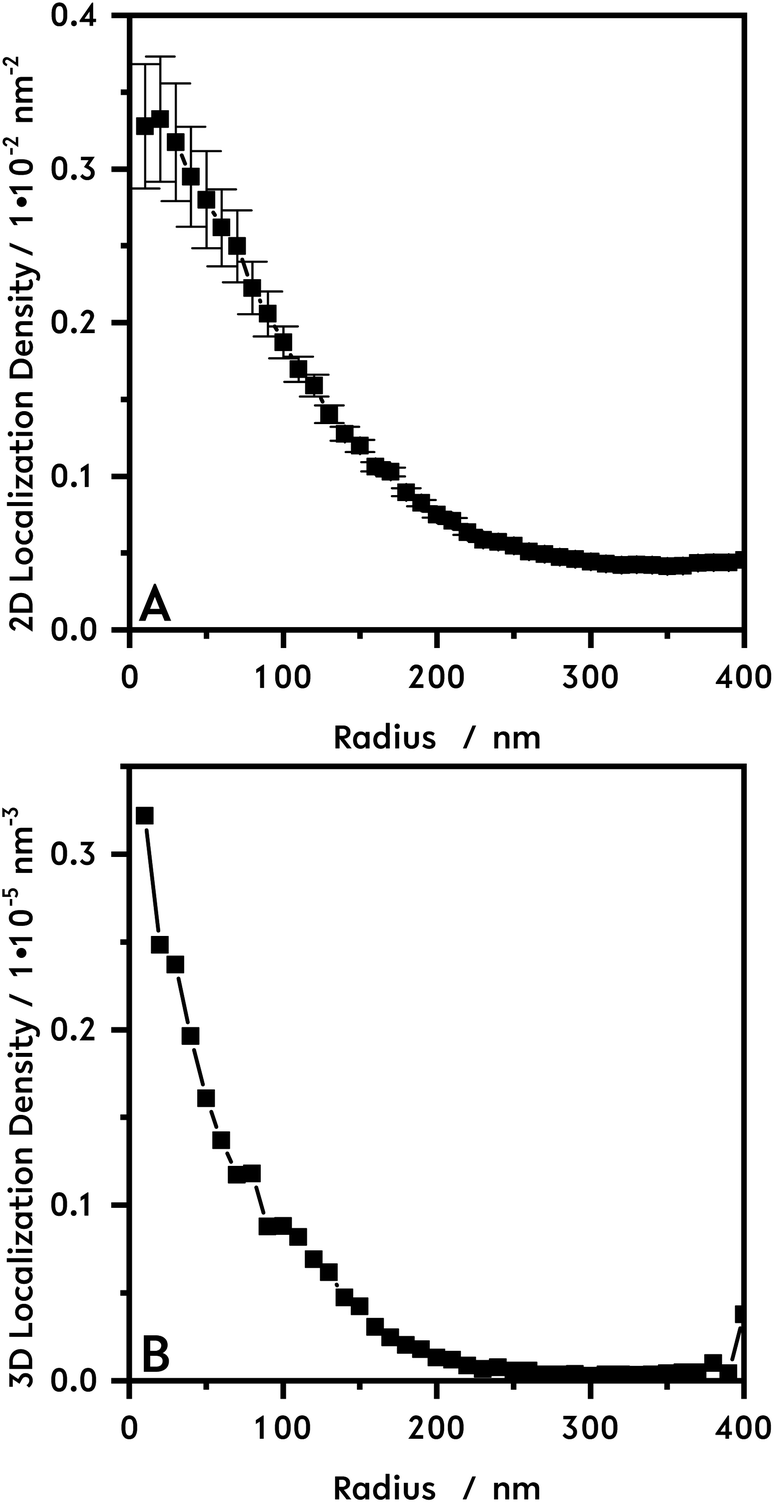
A sparse local density distribution of molecules in the fluorescent “on-state” is obtained by the application of a dSTORM imaging buffer containing an enzymatic oxygen scavenger system combined with a thiol, in this case 1 M cysteamine hydrochloride (M6500, Sigma Aldrich, USA) (MEA) adjusted to pH 7.4 with 25% hydrochloric acid or 1 M potassium hydroxide. The concentrations in the final buffer are 60 U mL−1 catalase (C100-50MG, Sigma Aldrich, USA), 5 U mL−1 glucose oxidase (G2133-10KU, Sigma Aldrich, USA) and 100 mM MEA. A small drop, typically 20 μL of the imaging buffer is added to the sample slide. The advantage of adding only a small drop to the slide is, that the remaining sample is not altered during the acquisition process of other spots on the cover glass. With the HILO illumination scheme the best results are obtained because the free floating R6G molecules above the microgels were not excited. To translate most of the fluorescent molecules to the long lived dark state, via the triplet state in combination with the thiol, a laser power density between 4 kW cm−2 and 5 kW cm−2 is applied to the sample. In total 20000 frames are acquired, where the imaging frequency for the core only microgels is set to 50 Hz and for the core–shell microgels to 30 Hz. For imaging of the swollen state of the microgel at 17 °C (see Fig. 1A and 3A, D, G) the objective plate is cooled down with an ice-pack, and the temperature is measured with a thermoelement (HH506RA, OMEGA, Germany) within the imaging buffer solution.
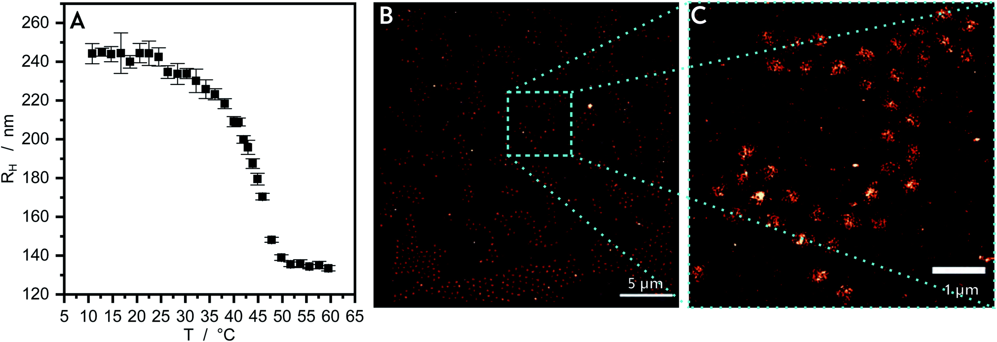 | ||
| Fig. 1 The temperature dependent swelling behaviour of microgels made of PNIPMAM, which are subsequently used as cores, is here characterized by PCS shown in (A). In (B) a dSTORM reconstruction of the microgels is presented, where (C) is the zoom-in of the cyan highlighted area in (B). | ||
2.6 Image reconstruction
000 images are divided into bins of 1000 frames and the resulting drift correction is smoothed with a factor of 0.25. For finding the single microgels an image with adjusted contrast and brightness is used to make it easier for the imfindcircle function to localize the single microgels. For the later evaluation the resulting localization table is used.
3 Computational methods
3.1 3D quantification of 2D projected single molecule localization microscopy data
For the quantification of the superresolved single molecule localization data that resulted from the experiments we use the drift corrected localization table and the resulting reconstructed image to identify the centre of the microgel by the built-in function imfindcircle, which provides the coordinates of the centre and the radius of the microgel based on the image. This function is also used to filter for spherical objects with a radius between 67.2 nm and 336 nm for the core microgels and between 224 nm and 448 nm for the core–shell microgels. From each localized centre the number of localizations in rings of 10 nm thickness is counted until a radius of 400 nm is reached. The final localization density of each ring is calculated by the total number of localizations in the ring divided by the ring area. The final localization density for the core and the core–shell microgels is shown in Fig. 4A, where the mean value is displayed with the standard error of the mean. From the 2D projection it's possible to recalculate a 3D density under the assumption that we consider a spherical object.With equally spaced rings of Δr = 10 nm the radial localization density profile consists of spherical shells of the same width. For the quantification a volume matrix Vsrij representing volume elements of the spherical shells is needed, where the outer shell radius r is defined as r = Rmax −Δri for each element and the width w = Δr(j + 1 + i). A cylinder with a radius of r − w and the height of r is cut out. The variable Rmax is defined during the localization density calculation and in this study is set to 400 nm, because of the particle size. The size of the matrix depends on the number of rings respective to the number of shells  . The matrix spans the dimension i × j, where i and j are running from 0 to n − 1:
 | (1) |
The localization density of each shell can be calculated by dividing the localizations of the ring of the projection belonging to this shell by the respective matrix volume element:
 | (2) |
 | (3) |
For i = 0 the equation simplifies to
| Nloc,shelli(r) = Nloc,proji(r). | (4) |
Therefore, the localization density for the shells is calculated from the outside to the inside. The final recalculation of the microgels is then shown in Fig. 4B. As a guide to the eye, normalized data are also provided, where the data for the core and the core–shell microgel is normalized to values between zero and one for the 2D projection (Fig. S6C†) and the 3D recalculation (Fig. S6D†).
4 Results and discussion
4.1 Measurements on the PNIPMAM core particles
The PNIPMAM core microgel particles are characterized as synthesized in aqueous suspension by photon correlation spectroscopy (PCS) (Fig. 1A) to determine the temperature-dependent hydrodynamic radius RH and the swelling behaviour. The PNIPMAM core particles contain a cross-linker content of 10 mol%. The PCS measurement is performed in a temperature range from 10 to 60 °C at a scattering angle of 45°. The data are analyzed by the CONTIN program. At low temperatures the particles are swollen and they have a RH of approximately 240 nm. At approximately 42 °C the core particles collapse and their hydrodynamic radius decreases to a plateau value of approximately 135 nm. This thermoresponsive behaviour is typical for an acrylamide-based microgel and the collapse of PNIPMAM in H2O can be seen at 42 °C.47,48 The collapsed and dried core particles are characterized by atomic force microscopy (AFM, Section S1†). In Fig. S1A† the AFM measurement of these particles are shown. The particles are identifiable as circular profiles with a low polydispersity.For the super-resolution fluorescence microscopy measurement the fluorescent dye Rhodamine 6G (R6G) is used. The PNIPMAM core microgel particles are mixed with an aqueous R6G solution for a few days. During the mixing time the dye molecules diffuse into the swollen polymer network due to favourable interactions. The nature of these interactions is still unclear. Coulomb or hydrophobic interactions are possible but the latter are more probable as indicated by measurements of Zhou et al. which showed the localization of the initiator charges in the area near the particle surface.49 After a few days this solution is diluted again, it is placed onto a cover glass coated with polyethylenimine by spin-coating and measured in an aqueous dSTORM-buffer. The R6G molecules freely diffuse into the microgel particles so that the “blinking” of single fluorophores can be recorded. The recorded frames are summed up to generate the reconstructed images.
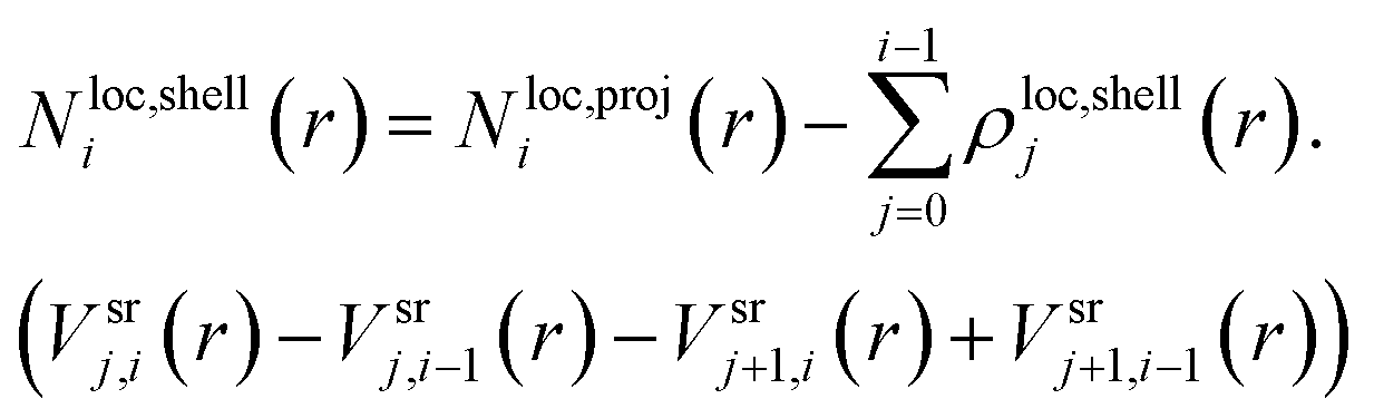
In Fig. 1B the dSTORM reconstruction image of the core microgel particles with the freely diffusing R6G are shown. Fig. 1C, shows an enlarged section of this image. In the background the localization density is almost zero. For the pure core particles the highest number of dye molecules is located in the middle of the particles. The 2D localization density of the pure core microgel particles (Fig. 2A) can be determined from the reconstructed image and the 3D localization density is recalculated (Fig. 2B). The localization density of the R6G fluorophores is highest in the middle of a core particle and decreases drastically with increasing particle radius. As already mentioned above, this is different compared to PNIPAM microgels which show a plateau or at least a large linear zone in the densities obtained from the inner part of the particles. In a previous study using AFM it was also shown that PNIPMAM microgels seem to exhibit a different network structure compared to PNNPAM and PNIPAM microgels.12 The size of a swollen core particle is found to be approximately 240 nm just as in the PCS measurement (see Fig. 1A). This is similar compared to our previous study and shows the approach is also useful to characterize the morphology of microgels based on different acrylamides.19
 | ||
| Fig. 2 In (A) the 2D localization density of the core microgel (N = 1048) is plotted following the calculation model shown in Fig. S5.† In (B) the recalculated 3D localization density is shown. | ||
4.2 Measurements on the core–shell system
The three different core–shell particles are analyzed analogously to the pure core particles. The PNNPAM shell contains a cross-linker content of 2 mol% for each of the three core–shell systems and different thicknesses (thin, intermediate and thick). In the swelling behaviour measured by PCS (Fig. 3A, D and G) of all of these three systems we observe three regions.14 In the first region at lower temperature all particles are in a swollen state with a hydrodynamic radius of 280–315 nm. The collapse of the PNNPAM shell is observable at approximately 21 °C.50 The difference in the hydrodynamic radius of the fully swollen microgel and the intermediate state with a collapsed shell and a still swollen core becomes larger from microgels with a thin to those with a thick shell. The second region shows a linear relation between the hydrodynamic radius and the temperature, which is caused by an interpenetration of the NNPAM shell material into the PNIPMAM core.16 The particle size decreases with increasing temperature. In the third region the particles are completely collapsed and the hydrodynamic radius reaches a plateau value of 170–180 nm. The structure of the shell region does not change. Core and shell show a thermoresponsive behaviour, which was also shown by Zeiser et al.14 and Cors et al.15 on comparable core–shell systems. The AFM measurements of the core–shell particles are shown in Fig. S1B–D.† Here, we can see the circularity in shape and a low polydispersity of the particles. In Fig. S8–S10† reconstructed 3D dSTORM images can be seen. A slight distortion from the spherical shape of the microgels at the solid liquid interface is observable. This was already reported by Hoppe Alvarez et al.51 and is due to interactions between the particles and the interface.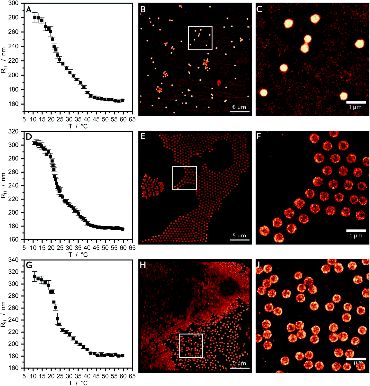 | ||
| Fig. 3 (A, D and G) show the swelling curves of the three core–shell microgels with nominally increasing shell thickness from thin, intermediate to thick. The shell thickness is varied according to the synthesis described in methods under 2.1. The reconstructed dSTORM images (B, E and H) for the microgels with different thick shells are shown in the remaining images with increasing shell thickness from the top to the bottom. Images on the right hand side (C, F and I) are the zoomed versions of the white highlighted regions of interest. | ||
In Fig. 3B, E and H the dSTORM reconstructed images of the core–shell microgel particles with freely diffusing R6G are shown. Fig. 3C, F, I and H show enlarged sections of these images. For the intermediate and thick shell (Fig. 3E, F and H, I) the highest intensity is seen in the shell region. For the thin shell (Fig. 1A and B) we observe a much higher intensity. In all of the images there is only a negligibly small intensity in the background.
In Fig. 4 the 2D (A) and 3D (B) localization densities of the core–shell particles with the three different shell thicknesses are shown. In the region of the theoretically collapsed core (up to 140 nm) the localization density differs strongly from the pure core particles. For the thin shell (Fig. 4, green triangle) a higher localization density can be seen which might be caused by a higher interaction of R6G with the core–shell system containing PNNPAM, as the sum of all localizations is higher for the collapsed-core region of the thin shell system as for the complete core particles. An alternative explanation to a compressed core is the interpenetration of the monomer NNPAM into the collapsed core during the synthesis. This is in good agreement with recent small angle neutron scattering (SANS) results using contrast variation.16 The NNPAM content increases from the inside to the outside, due to the inhomogeneous cross-linker density of the core, so that outside of the core region only NNPAM is swollen. For higher shell densities (see Fig. 4, intermediate: yellow circle, thick: blue triangle) almost no dye localization in the core region is observed. The intensity in the core region is negligibly small due to the fact that the core can no longer be reached for R6G fluorophores. Based on SANS results this observation leads to the conclusion that due to the strong interpenetration the particles are rather dense inside and the dye only penetrates the shell in these microgels.16
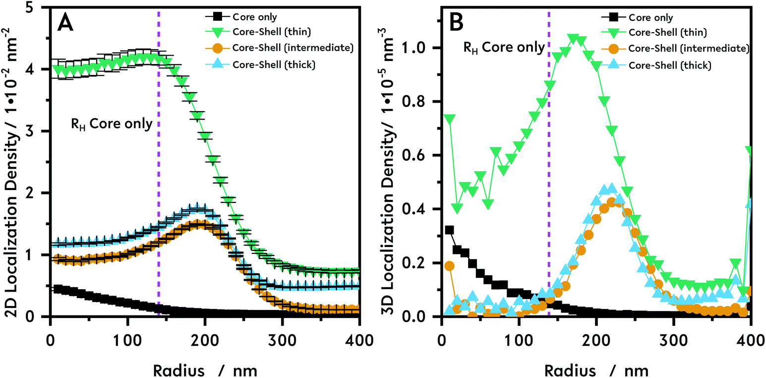 | ||
| Fig. 4 The microgels are immersed in R6G solutions and afterwards spincast on PEI coated cover slips. To remove excess dye molecules the sample is washed with purified water while spincasting. The remaining dye molecules in the microgels are localized. We investigated the localization densities, acquired by dSTORM, of core–shell microgels with three different shell thicknesses termed as “thin” (green triangle, N = 314), “intermediate” (yellow circle, N = 608) and “thick” (blue triangle, N = 1512) with a cross-linker content of 10 mol% for the core and 2 mol% for the shell during the synthesis. Therefore, the presented scheme for data evaluation (see Fig. S5†), after getting the localization table, is used. Localizations are counted and assigned to circular rings with a width of 10 nm. From this it's possible to calculate a localization density for each ring. This was done for the core and the three different core–shell microgels. The 2D localization density shown in (A) shows a higher localization density for all the core–shell microgels over the whole radius in comparison to the core microgel. In (B) the recalculated 3D density for all measured microgels is shown. The hydrodynamic radius RH of the collapsed core microgels is indicated by the dashed line in magenta in both graphs. | ||
5 Conclusion
Recently, we presented a quantitative method to characterize the network density of N-isopropylacrylamide (NIPAM) based microgels by means of localization of freely diffusing probes.19 The method has reproduced the established density distribution of a fuzzy sphere11 for well studied NIPAM microgels with 5 mol% N,N′-methylenebisacrylamide (BIS) as cross-linker. Furthermore, for highly crosslinked NIPAM microgels with 7.5 and 10 mol% BIS, respectively, a deviation from the fuzzy sphere model could be found and a correction with an additional linear term was proposed. In the present study we demonstrate, that this method can also be applied to core–shell microgel particles made of two different acrylamides.In this work the internal morphology of PNIPMAM core microgel and PNIPMAM-PNNPAM core–shell microgels are studied by super-resolution fluorescence microscopy. We investigate core–shell systems with three different PNNPAM shell thicknesses. As fluorescent dye for dSTORM measurements we use freely diffusing rhodamine 6G, so the localization density inside the particles can be determined. For initial core microgel particles the fluorescent dye diffuses into the particles and the fluorophores are located in the microgel particles. For core–shell particles the NNPAM shell material interpenetrates the PNIPMAM core. The interpenetration results in a higher localization density due to an increased interaction between the fluorophores and the polymer network. For thicker shells a higher degree of interpenetration can be observed as almost no localization is found in the core of the core–shell particles. We hypothesize that this might be either due to an increase in network density due to interpenetration of the shell polymer into the core, which prohibits the diffusion of the fluorophores into the polymer network or the formation of a diffusion barrier. The thicker shell also inhibits the diffusion of the fluorophores into the core, such that just a small amount of fluorophores can be found in the core region. Furthermore, the interpenetration of the shell material into the core is high enough that dye molecules in a size range of rhodamine 6G molecules are not able to reach the core. This work has potential implications for studies, where microgels are loaded with small molecules, e.g. in drug delivery. Moreover, it shows that the use of freely diffusing probe molecules is promising for a broader range of soft colloidal systems.
Conflicts of interest
There are no conflicts to declare.Acknowledgements
This research was supported by the Bielefelder Nachwuchsfond of Bielefeld University. We are grateful to Robin Diekmann, EMBL Heidelberg, Germany, for help with the Superresolution Microscopy Analysis Platform (SMAP) and fruitful discussions on how to find the best reconstruction parameters. We thank Ina Ehring for her help with the syntheses.References
- R. Pelton, Adv. Colloid Interface Sci., 2000, 85, 1–33 CrossRef CAS.
- S. Nayak and L. A. Lyon, Angew. Chem., Int. Ed., 2005, 44, 7686–7708 CrossRef CAS.
- W. Richtering and B. R. Saunders, Soft Matter, 2014, 10, 3695–3702 RSC.
- M. Karg, A. Pich, T. Hellweg, T. Hoare, L. A. Lyon, J. J. Crassous, D. Suzuki, R. A. Gumerov, S. Schneider, I. I. Potemkin and W. Richtering, Langmuir, 2019, 35, 6231–6255 CrossRef CAS.
- J. K. Oh, R. Drumright, D. J. Siegwart and K. Matyjaszewski, Prog. Polym. Sci., 2008, 33, 448–477 CrossRef CAS.
- B. R. Saunders, N. Laajam, E. Daly, S. Teow, X. Hu and R. Stepto, Adv. Colloid Interface Sci., 2009, 147–148, 251–262 CrossRef CAS.
- Q. M. Zhang, W. Xu and M. J. Serpe, Angew. Chem., Int. Ed., 2014, 53, 4827–4831 CrossRef CAS.
- C. D. Sorrell and M. J. Serpe, Anal. Bioanal. Chem., 2012, 402, 2385–2393 CrossRef CAS.
- K. Uhlig, T. Wegener, J. He, M. Zeiser, J. Bookhold, I. Dewald, N. Godino, M. Jaeger, T. Hellweg, A. Fery and C. Duschl, Biomacromolecules, 2016, 17, 1110–1116 CrossRef CAS.
- K. Uhlig, T. Wegener, Y. Hertle, J. Bookhold, M. Jaeger, T. Hellweg, A. Fery and C. Duschl, Polymers, 2018, 10, 656 CrossRef.
- M. Stieger, W. Richtering, J. S. Pedersen and P. Lindner, J. Chem. Phys., 2004, 120, 6197–6206 CrossRef CAS.
- B. Wedel, Y. Hertle, O. Wrede, J. Bookhold and T. Hellweg, Polymers, 2016, 8, 162 CrossRef.
- O. Wrede, Y. Reimann, S. Lülsdorf, D. Emmrich, K. Schneider, A. J. Schmid, D. Zauser, Y. Hannappel, A. Beyer, R. Schweins, A. Gölzhäuser, T. Hellweg and T. Sottmann, Sci. Rep., 2018, 8, 13781 CrossRef.
- M. Zeiser, I. Freudensprung and T. Hellweg, Polymer, 2012, 53, 6096–6101 CrossRef CAS.
- M. Cors, O. Wrede, A.-C. Genix, D. Anselmetti, J. Oberdisse and T. Hellweg, Langmuir, 2017, 33, 6804–6811 CrossRef CAS.
- M. Cors, O. Wrede, L. Wiehemeier, A. Feoktystov, F. Cousin, T. Hellweg and J. Oberdisse, Sci. Rep., 2019, 9, 13812 CrossRef.
- L. Wiehemeier, M. Cors, O. Wrede, J. Oberdisse, T. Hellweg and T. Kottke, Phys. Chem. Chem. Phys., 2019, 21, 572–580 RSC.
- A. P. H. Gelissen, A. Oppermann, T. Caumanns, P. Hebbeker, S. K. Turnhoff, R. Tiwari, S. Eisold, U. Simon, Y. Lu, J. Mayer, W. Richtering, A. Walther and D. Wöll, Nano Lett., 2016, 16, 7295–7301 CrossRef CAS.
- S. Bergmann, O. Wrede, T. Huser and T. Hellweg, Phys. Chem. Chem. Phys., 2018, 20, 5074–5083 RSC.
- S. T. Hess, T. P. K. Girirajan and M. D. Mason, Biophys. J., 2006, 91, 4258–4272 CrossRef CAS PubMed.
- M. Heilemann, S. van de Linde, M. Schüttpelz, R. Kasper, B. Seefeldt, A. Mukherjee, P. Tinnefeld and M. Sauer, Angew. Chem., Int. Ed., 2008, 47, 6172–6176 CrossRef CAS.
- A. Sharonov and R. M. Hochstrasser, Proc. Natl. Acad. Sci. U. S. A., 2006, 103, 18911–18916 CrossRef CAS.
- A. Purohit, S. P. Centeno, S. K. Wypysek, W. Richtering and D. Wöll, Chem. Sci., 2019, 50, 131 Search PubMed.
- A. Aloi, N. Vilanova, L. Albertazzi and I. K. Voets, Nanoscale, 2016, 8, 8712–8716 RSC.
- O. Nevskyi, D. Sysoiev, J. Dreier, S. C. Stein, A. Oppermann, F. Lemken, T. Janke, J. Enderlein, I. Testa, T. Huhn and D. Wöll, Small, 2018, 14, 1703333 CrossRef.
- E. Siemes, O. Nevskyi, D. Sysoiev, S. K. Turnhoff, A. Oppermann, T. Huhn, W. Richtering and D. Wöll, Angew. Chem., Int. Ed., 2018, 57, 12280–12284 CrossRef CAS.
- A. A. Karanastasis, Y. Zhang, G. S. Kenath, M. D. Lessard, J. Bewersdorf and C. K. Ullal, Mater. Horiz., 2018, 5, 1130–1136 RSC.
- L. Etchenausia, E. Villar-Alvarez, J. Forcada, M. Save and P. Taboada, Mater. Sci. Eng., C, 2019, 104, 109871 CrossRef.
- X. Zhou, F. Chen, H. Lu, L. Kong, S. Zhang, W. Zhang, J. Nie, B. Du and X. Wang, Ind. Eng. Chem. Res., 2019, 58, 10922–10930 CrossRef CAS.
- D. Yang, M. Viitasuo, F. Pooch, H. Tenhu and S. Hietala, Polym. Chem., 2018, 9, 517–524 RSC.
- R. H. Pelton and P. Chibante, Colloids Surf., 1986, 20, 247–256 CrossRef CAS.
- T. Hirano, K. Nakamura, T. Kamikubo, S. Ishii, K. Tani, T. Mori and T. Sato, J. Polym. Sci., Part A: Polym. Chem., 2008, 46, 4575–4583 CrossRef CAS.
- S. W. Provencher, Comput. Phys. Commun., 1982, 27, 213–227 CrossRef.
- S. W. Provencher, Comput. Phys. Commun., 1982, 27, 229–242 CrossRef.
- D. Axelrod, T. P. Burghardt and N. L. Thompson, Annu. Rev. Biophys. Bioeng., 1984, 13, 247–268 CrossRef CAS PubMed.
- M. Tokunaga, N. Imamoto and K. Sakata-Sogawa, Nat. Methods, 2008, 5, 159–161 CrossRef CAS PubMed.
- R. Diekmann, K. Till, M. Müller, M. Simonis, M. Schüttpelz and T. Huser, Sci. Rep., 2017, 7, 14425 CrossRef.
- H. P. Babcock, Sci. Rep., 2018, 8, 1726 CrossRef PubMed.
- A. Sandmeyer, M. Lachetta, H. Sandmeyer, W. Hübner, T. Huser and M. Müller, DMD-based super-resolution structured illumination microscopy visualizes live cell dynamics at high speed and low cost, 2019, vol. 9, DOI:10.1101/797670.
- M. Müller, V. Mönkemöller, S. Hennig, W. Hübner and T. Huser, Nat. Commun., 2016, 7, 10980 CrossRef.
- B. Huang, W. Wang, M. Bates and X. Zhuang, Science, 2008, 319, 810–813 CrossRef CAS.
- K. J. A. Martens, A. N. Bader, S. Baas, B. Rieger and J. Hohlbein, J. Chem. Phys., 2018, 148, 123311 CrossRef PubMed.
- D. Sage, T.-A. Pham, H. Babcock, T. Lukes, T. Pengo, J. Chao, R. Velmurugan, A. Herbert, A. Agrawal, S. Colabrese, A. Wheeler, A. Archetti, B. Rieger, R. Ober, G. M. Hagen, J.-B. Sibarita, J. Ries, R. Henriques, M. Unser and S. Holden, Nat. Methods, 2019, 313, 1642 Search PubMed.
- Y. Li, M. Mund, P. Hoess, J. Deschamps, U. Matti, B. Nijmeijer, V. J. Sabinina, J. Ellenberg, I. Schoen and J. Ries, Nat. Methods, 2018, 15, 367–369 CrossRef CAS PubMed.
- A. Markwirth, M. Lachetta, V. Mönkemöller, R. Heintzmann, W. Hübner, T. Huser and M. Müller, Nat. Commun., 2019, 10, 4315 CrossRef PubMed.
- M. Ovesný, P. Křížek, J. Borkovec, Z. Svindrych and G. M. Hagen, Bioinformatics, 2014, 30, 2389–2390 CrossRef PubMed.
- I. Berndt, C. Popescu, F.-J. Wortmann and W. Richtering, Angew. Chem., Int. Ed., 2006, 45, 1081–1085 CrossRef CAS PubMed.
- B. Wedel, M. Zeiser and T. Hellweg, Z. Phys. Chem., 2012, 226, 737–748 CrossRef CAS.
- J. Zhou, J. Wei, T. Ngai, L. Wang, D. Zhu and J. Shen, Macromolecules, 2012, 45, 6158–6167 CrossRef CAS.
- D. Ito and K. Kubota, Polym. J., 1999, 31, 254–257 CrossRef CAS.
- L. Hoppe Alvarez, S. Eisold, R. A. Gumerov, M. Strauch, A. A. Rudov, P. Lenssen, D. Merhof, I. I. Potemkin, U. Simon and D. Wöll, Nano Lett., 2019 DOI:10.1021/acs.nanolett.9b03688.
Footnotes |
| † Electronic supplementary information (ESI) available: Experimental details and results for atomic force microscopy done for the core and core–shell microgels. Additional details and results for the dSTORM experiments. See DOI: 10.1039/c9na00670b |
| ‡ These authors contributed equally to this work. |
| This journal is © The Royal Society of Chemistry 2020 |