Spatial focusing of magnetic particle hyperthermia

Abstract

Magnetic particle hyperthermia is a promising cancer therapy, but a typical constraint of its applicability is localizing heat solely to malignant regions sparing healthy surrounding tissues. By simultaneous application of a constant magnetic field together with the hyperthermia inducing alternating magnetic field, heating focus may be confined to smaller regions in a tunable manner. The main objective of this work is to evaluate the focusing parameters, by adequate selection of magnetic nanoparticles and field conditions, and explore spatially focused magnetic particle hyperthermia efficiency in tissue phantom systems comprising agarose gel and magnetic nanoparticles. Our results suggest the possibility of spatially focused heating efficiency of magnetic nanoparticles through the application of a constant magnetic field. Tuning of the constant magnetic field parameters may result in minimizing thermal shock in surrounding regions without affecting the beneficiary thermal outcome in the focusing region.

---

Introduction

Hyperthermia is widely accepted as an adjuvant cancer treatment modality, offering several modes for heating, such as microwaves, photodynamic therapy, radio frequency, and ultrasound with different success rates.^1–5 The approach of combining an external radiofrequency electromagnetic field with magnetic nanoheating carriers, widely known as magnetic particle hyperthermia (MPH), is a strong candidate with great prospects.^6–8 Materials research on magnetic hyperthermia agents is mainly devoted to iron oxide nanoparticles because they are biocompatible and they follow a well-known metabolic pathway in the human body.^9,10 Specifically, iron oxide magnetic nanoparticles with superparamagnetic behaviour (MLF AS, MagForce Nanotechnologies AG, Berlin, Germany, 15 nm) have been approved for clinical trials on patients with glioblastoma multiforme^11–14 or prostate cancer.^15,16 In addition, MNPs may be used in multifunctional aspects in medical imaging and provide important information for diagnosis and therapy.^17–19 Currently, there are five commercially available MNP preparations exploited in magnetic particle imaging (MPI) such as Perimag (micromod Partikeltechnologie, Rostock, Germany), FerraSpin-R (nanoPET-Pharma, Berlin, Germany), fluidMag-D 50 (chemicell, Berlin, Germany), Ferucarbotran (Meito Sangyo, Nagoya, Japan) and SEONLA-BSA (SEON group, Erlangen, Germany).²⁰ Earlier applications of MPI focused on vascular imaging such as 3D imaging of a beating mouse heart using commercial nanoparticle suspensions, like Resovist, composed of super-paramagnetic iron oxide MNPs.²¹ Furthermore, studies have shown that synergies between magnetic particle imaging and magnetic hyperthermia goes through the design of better scanners and an improvement of the current resolution.^22,23 Thus, magnetic nanoparticles make themselves most important candidates in cancer diagnosis and treatment in MPI and magnetic hyperthermia, respectively.²⁴

Since a typical problem in the implementation of magnetic particle hyperthermia is its difficulty to selectively localize heat without potentially damaging the surrounding healthy tissues, experimental work has been directed towards the concept of constant magnetic field application (currently employed in MPI), in order to reduce the risk of overheating the healthy tissues while potentially proposing a novel multifunctional (MPI + MPH) theranostic platform.^25,26 Moreover, Murase et al. studied the role of a constant magnetic field applied in magnetic resonance imaging (MRI) in combination with MPH in order to target the MNPs in specific areas deep in a body. They found that combining MRI and MPH may increase the efficiency of the latter, due to the temperature rise being controlled by the constant magnetic field of MRI reducing the damage in healthy tissues.²⁷ Theoretical studies have also shown that the presence of a constant magnetic field may affect MPH features.^28,29 The heat generation mechanism can be fine-tuned by varying the alternating magnetic field amplitude with respect to the concurrent application of a constant magnetic field (constant magnetic field). A small magnetic field, of only 40 mT, appears sufficient to cancel out the heating effect of the nanoparticles.³⁰ However, most of the studies to date are limited only to superparamagnetic particles, without evaluating the parameters to tune spatial heating e.g. by varying the size of MNPs. Particle size is a crucial efficiency moderator in hyperthermia.^31–36 With respect to MNP size, the magnetic heating efficiency mechanism relies on hysteresis and/or relaxational losses when MNPs are subjected to an alternating current (AC) magnetic field.³⁷ As the size of MNPs increases, a coercivity field together with magnetization evolves giving rise to much stronger field–particle interactions. Eventually, the heating efficiency may amplify by switching from superparamagnetic to ferromagnetic particles, for which a well-defined hysteresis loop area is formed.^38,39 Ultimately, on the clinical side, a key challenge is to have a reliable and versatile temperature monitoring system. Here, we present a method for obtaining a spatial thermal distribution by incorporating a constant magnetic field setup into a typical MPH system as depicted in Fig. 1.

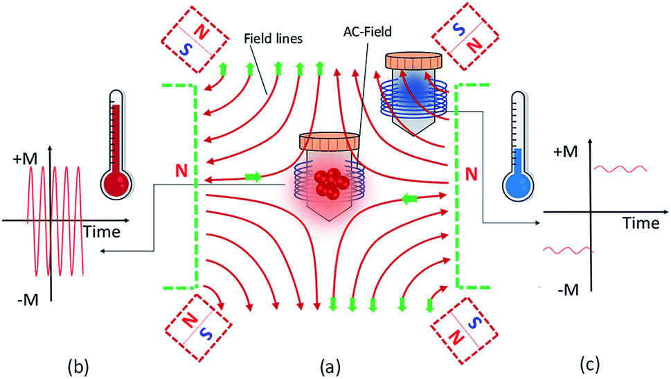Fig. 1 Schematic diagram of the experimental setup for alternating and constant magnetic fields. (a) Alternating field is generated by a commercial inductive heater while the constant magnetic field is generated by a setup of NdFeB permanent magnets. Constant magnetic field lines are illustrated with red lines. There are two possible positions of magnets (cubic-red colour or rectangular-green colour) which are illustrated with the dashed lines. Left (b) and right (c) magnetization graphs corresponding to magnetization variations with time with respect to sample localization either in the central field free (FFR) region (b) or (c) in the surrounding area where the AC and constant magnetic field are coexisting.

A setup of 2 or 4 commercial NdFeB magnets fixed on a clear perspex plate creates the constant magnetic field. The outline of the permanent magnets is illustrated with dashed lines in Fig. 1. The setup may be placed on or off centre of the sample vessel surrounded by the hyperthermia coil, generating the AC field. In either case the sample is subjected to the addition of the two field vectors (AC and constant magnetic field). The direction of the magnetic field is shown in Fig. 1a with solid line arrows. The green colour corresponds to the rectangular magnets while the red colour to the cubic magnets. In the central region, the constant magnetic field magnitude may be attenuated according to magnet arrangement and an area where its value may be safely approximated to zero arises. This area is called the field free region (FFR). It is possible to change the FFR geometry using an appropriate number of magnets, field magnitude and orientation. By the simultaneous application of the AC and constant magnetic fields, the spatial thermal distribution may be realized in two areas as follows: (1) FFR area, where the constant magnetic field is zero, and (2) saturation region (SR area), where the constant magnetic field is maximum. In the FFR region, MNPs experience solely the AC hyperthermia field, resulting in maximum AC heating. The magnetization of MNPs can oscillate between +M and −M at the AC magnetic field frequency and allow the delivery of heat to their surroundings (Fig. 1b). The magnetization of MNPs can change only in response to the AC field, because the constant magnetic field is so weak in the FFR region, causing maximum heating efficiency. In contrast, in the SR area, where the sample is off the FFR region and closer to the magnets, the oscillating field does not significantly change the magnetization of the MNPs, which remains saturated (Fig. 1c). The constant magnetic field is strong enough to keep the MNP magnetization in a saturated state. This situation results in a minimal energy release by the MNPs.

The specific loss power index (SLP) is a quantifiable measure of the heating efficiency of MNPs and will be used to evaluate the heating response of the systems under study. In all cases, we selected to use phantom systems consisting of agarose gel with MNPs homogenously dispersed, mimicking human tissues, to have a more realistic performance perspective.

In order to study the efficiency of a focused magnetic particle hyperthermia system, we examine the SLP variations in two different geometrical magnetic configurations and on three different phantom samples based on three iron oxide (Fe₃O₄) magnetic nanoparticle systems namely 10, 40 and 80 nm. Thus, we will be able to provide information of the focusing effect for the three major MNP categories, i.e., superparamagnetic (SPM), single-domain (SD), and multi-domain (MD).⁸ Despite the fact that the distinction between the three regions is not sharp, we may safely regard the 10 nm MNPs as a typical SPM system, the 40 nm MNPs as a typical SD system and the 80 nm MNPs as an MD system. The FFR and SR areas are presented for two different configurations of constant magnetic fields while the MNP heating efficiency is studied when AC and constant magnetic fields are applied simultaneously. This study provides a principle for the heating of an adaptable spatial area inside a biological body. This may be exploitable with necessary modifications in clinical practice in the future, making magnetic hyperthermia a modern cancer treatment modality by achieving controllable heating while sparing healthy tissues.

Experimental

Synthesis and characterization

Magnetic particle hyperthermia experimental sequences were carried out on phantom samples, comprising magnetic nanoparticles dispersed in an agarose matrix. Initially, three different iron oxide NPs with average core diameters of 10, 40 and 80 nm were synthesized by the aqueous co-precipitation of ferric and ferrous salts under alkaline conditions at high temperature, as previously described.⁴⁰ It should be noted that the influence of the anions on the formation of iron oxides and the reagents used has a significant impact on size increase, creating iron oxide MNPs from 10 to 80 nm in diameter. Secondly, the designated mixture of the iron oxide MNPs (4 mg) and agarose (10 mg) was dissolved in 1 mL of deionized water, sonicated for three minutes and then placed in a water bath of 84 °C for ten minutes, so agarose could fully liquify and the sample could get homogenized under continuous stirring with respect to the MNP distribution. Finally, the solution was left to cool down under ambient conditions to provide agarose samples of 10 mg mL⁻¹ with a concentration of 4 mg mL⁻¹ iron oxide MNPs.

Magnetic hyperthermia

The magnetic particle hyperthermia experiments were performed using a 1.2 kW Ambrell Easyheat 0112 system providing alternating magnetic fields of 375 kHz and variable amplitudes between 10 and 70 mT. During the experimental sequence, the temperature was recorded every 0.4 s by using a GaAs-based fibre optic probe immersed in the sample. Eqn (1) estimates the heating efficiency of nanoparticles quantified in terms of specific loss power index (SLP), which determines the power dissipation per unit mass of magnetic material (in W g⁻¹) by using the following formula and a rigorous standardized procedure:⁴¹where c_p is the volume specific heat capacity of the sample, m_f the mass of the dispersion, m_MNPs is the MNP mass and ΔT/Δt is the value of the maximal slope at the initial time after switching on the alternating magnetic field.

Computational procedures

In order to evaluate and visualize the FFR parameters of the two different experimental setups we used a finite element method to simulate the constant magnetic field distribution. The two different experimental configurations of permanent NdFeB magnets⁴² capable of generating a strong constant magnetic field were simulated by using commercial software COMSOL Multiphysics (v.3.5a). The first 3D geometric model comprised two rectangular parallelepiped magnets (4.5 × 3 × 1 cm³) placed opposite to each other, while the second was a quadrupole with four cubic magnets (2 × 2 × 2 cm³). The “AC/DC magneto-statics, no currents” application mode, which handles magnetic fields without currents,⁴³ was used for calculating the resulting magnetic flux density in a 3D computational domain. When no currents are present, the problem is easier to solve using the magnetic scalar potential V_m related to the permanent magnet magnetic field H using the formula H = −∇V_m.⁴⁴ At the boundaries of the computational domain, we apply the magnetic insulation condition that sets the normal component of the magnetic flux density B to zero. This boundary condition is useful at these boundaries confining a surrounding region of air while the continuity boundary condition was applied at the magnet boundaries. This is the natural boundary condition ensuring the continuity of B in all the computational domains studied.⁴⁵ This application mode solves the equation

∇B = 0 ⇒ −∇·(μ₀μ_r∇V_m − B_r) = 0 (2)

where μ₀ is the permeability of vacuum, μ_r is the relative permeability of the NdFeB magnet which is equal to 1.05,⁴⁶ and B_r is the remnant magnetic flux density varying from 0 to 1.2 T, from the outside to the inside of the magnet, respectively. This equation assumes the following constitutive relationship between B and H

B = μ₀μ_rH + B_r (3)

By implementing this method, we visualize the spatial distribution of the magnetic field magnitude and direction, together with the position of the FFR, which is defined as the region where the magnetic field magnitude is more than two orders of magnitude lower than the maximum magnetic field observed on the edge of the magnets.

Results and discussion

Structure and magnetism

Transmission electron microscopy (TEM) imaging was used to examine the morphology and the polydispersity of the synthesized MNPs. More specifically, we found out that the average particle diameters of the three samples were 10 ± 2 nm, 40 ± 5 nm and 80 ± 10 nm. As we have observed in a series of TEM images, MNPs are roughly spherical (Fig. 2a) and with respect to their size we may have bigger discrepancies in the shape as aggregates are formed (Fig. 2b and c), due to the aqueous co-precipitation method of synthesis and the absence of surfactants during it.⁴⁷ In addition, X-ray diffraction patterns (XRD), shown in Fig. 2d, outline the existence of iron oxide typical reflections detected in all cases.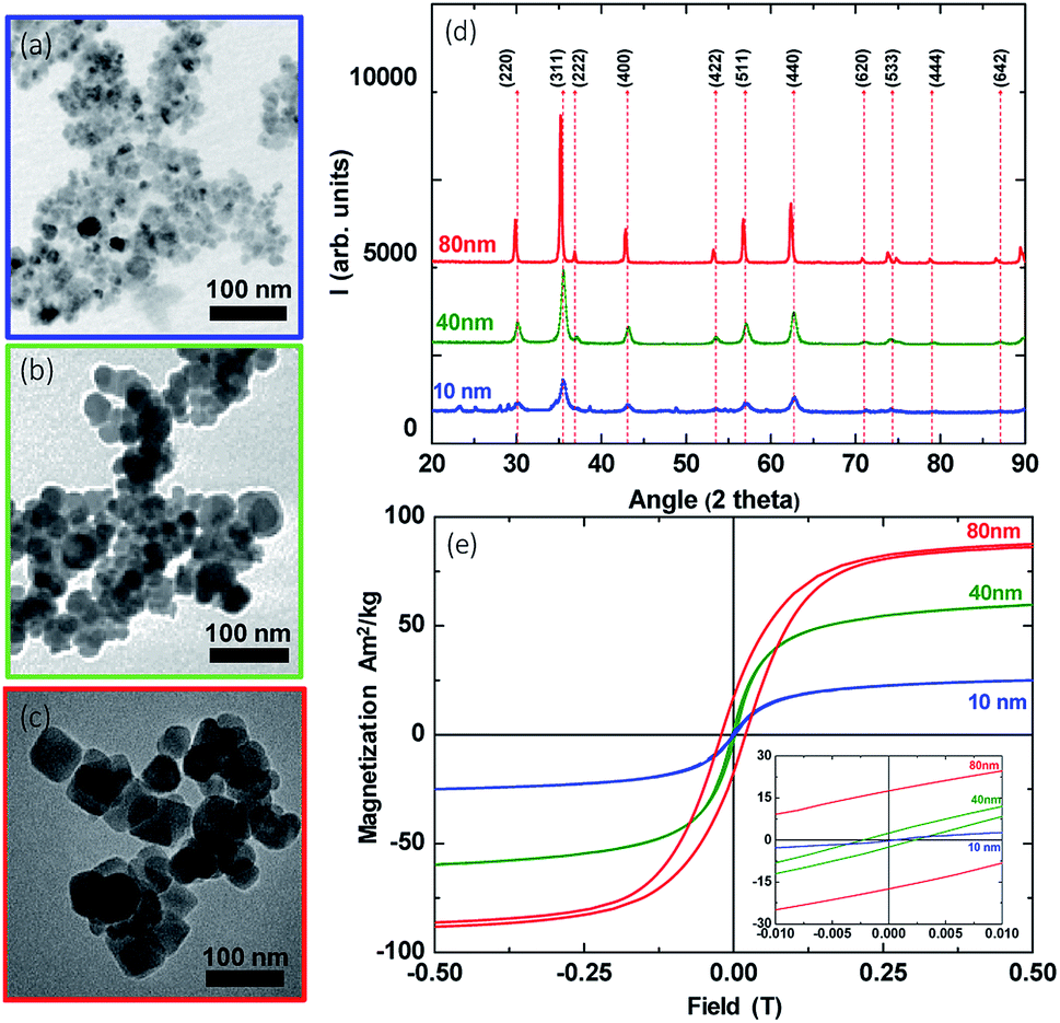

Fig. 2 Transmission electron microscopy (TEM) images of nanoparticles with average diameters 10, 40 and 80 nm are shown in (a), (b) and (c), respectively. The XRD diffraction patterns show the characteristic peaks of the iron oxide Fe₃O₄ crystal structure for all samples (d). The hysteresis loops recorded at room temperature. The inset shows a central region zoom of the hysteresis loop (e).

Room-temperature hysteresis loops were recorded in order to analyse the magnetic features of MNPs. As depicted in Fig. 2e, growing the size of MNPs resulted in an increased magnetic saturation M_s from 27 A m²/kg to 88 A m²/kg, approaching a corresponding bulk value of ∼90 A m²/kg.⁴⁸ Another important parameter, which determines the magnetic features, is the coercivity field H_c. H_c also increases with the MNP size. More specifically, it reaches a maximum value of 0, 2, and 20 mT for the MNPs with sizes 10, 40 and 80 nm, respectively, as shown in the inset of Fig. 2e. These results suggest that, as initially assumed, the 10 and 40 nm MNPs exhibited SPM and SD behaviour, respectively, in good agreement with relevant review studies.^8,49,50 Additionally, 80 nm MNPs safely reside within the MD region, with respect to their magnetization and coercivity as relevant studies on iron oxide MNPs have reported.⁵¹

Magnetic particle hyperthermia

Size effects. The magnetic features of MNPs are crucial parameters since they directly affect hysteresis losses which in turn may govern magnetic heating efficiency. Fig. 3 shows the experimental results of the heating efficiency for various values of the AC field (40, 50, 60 and 70 mT) for the three phantom samples. In this case, the frequency was kept constant at 375 kHz. The experimental results show that the SLP value is proportional to the applied magnetic field strength and the MNPs with a bigger size possess higher SLP values.

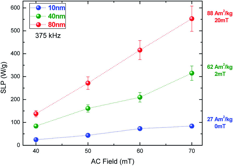Fig. 3 Heating efficiency expressed by SLP value dependence on the hyperthermia field amplitude for different diameters of iron oxide MNPs (blue – 10 nm, green – 40 nm and red – 80 nm) at a frequency of 375 kHz. On the right vertical axis, saturation magnetization and coercivity values are given for each MNP diameter.

To unravel the heating efficiency, we correlate the results with the magnetic measurements. In the case of small particles, namely 10 nm, the heating efficiency increases from 25 to 85 W g⁻¹ depending on the field. The magnetization is lower than the bulk magnetite and the H_c value is zero. That means that the SLP values are below 100 W g⁻¹ even under the maximum applied dominant phase. MNPs present no hysteresis, as expected, and their heating mechanism is mainly attributed to relaxation losses.⁵² This result is qualitatively similar to what has been reported in previous studies, which have shown that the SLP values are very low due to the small size.^40,53 If we increase the size from 10 to 40 nm, the SLP value becomes approximately four times higher. More specifically it varies from 80 to 320 W g⁻¹ for the lower and higher fields, respectively. Additionally, the two-fold magnetization increase from 27 to 62 A m²/kg, due to the SD behaviour, is apparent. Nemati et al. have shown the same behaviour for nanoparticles with a diameter of approximately 54 nm.⁵⁴

We can observe that in the MNPs with the biggest size (80 nm) the magnetization reaches a maximum value of 88 A m²/kg, due to the MD behaviour, increasing the SLP values to reach 110 to 550 W g⁻¹ for AC field amplitudes of 40 to 70 mT, respectively. These results indicate that the key to controlling the heating efficiency is the magnetization of MNPs. Such relationships between the MNP magnetic behaviour and heating efficiency have also been reported in previous studies, where the linearity between the hysteresis loop area and SLP value is verified both theoretically^55,56 and experimentally.^57–59

Combinations of AC and constant magnetic fields. The two different permanent magnet arrangements shown in Fig. 1 result in diverse spatial magnetic flux density distributions, which include FFRs of different sizes and shapes, as shown in Fig. 4, which depicts on a logarithmic scale the normalized to maximum magnetic flux density distributions.

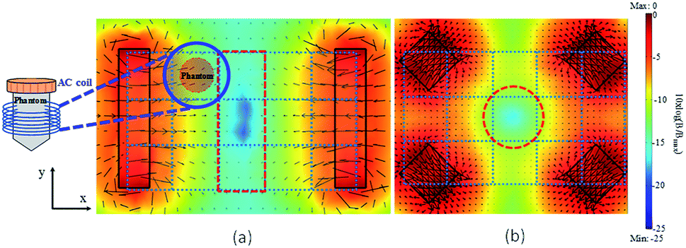Fig. 4 Simulation of the constant magnetic field configurations used to achieve spatially focused magnetic particle hyperthermia. (a) Two rectangular parallelepipeds, permanent NdFeB magnets, and (b) four cubic permanent NdFeB magnets. The rainbow-colored shades represent the normalized to maximum magnetic flux density given on a logarithmic scale (dB), while the black arrows depict the direction of magnetic field lines. The workspace (3 × 5 dotted squares corresponding to an area of 8 × 5 cm²) is located between the magnets and is outlined with (blue) dotted lines. The workspace includes the FFR, which is drawn with a (red) dashed line. The constant magnetic field setup may be adequately positioned so that the sample is eventually centred in any of the 15 different workspace squares and subjected to both AC and constant magnetic fields.

As shown in Fig. 4, the workspace is an 8 × 5 cm² area split into fifteen regions (x-y axis) according to the visualized geometry of the FFR. An appropriate alternating field inside the circular area may be simultaneously applied. Thus, the phantom sample was moved within the workspace at 15 spots to undergo combinatory field applications.

The coloured scale bar in Fig. 4 corresponds to the magnetic flux density of the constant magnetic field, on a logarithmic scale, while the black arrows correspond to the magnetic flux density vectors.

In the first field configuration (Fig. 4a), two rectangular shaped magnets (4.5 × 3 × 1 cm³) are placed 8 cm apart facing each other. Total magnetic flux density values were estimated numerically by using Comsol Multiphysics v. 3.5a, showing the occurrence of an area with practically zero constant magnetic field (a value of −25 dB which corresponds to a two orders of magnitude decrease with respect to the magnetic field value on magnet's edges), the so-called FFR. In Fig. 4b an alternative setup of four cubic magnets (2 × 2 × 2 cm³) is used resulting in a different FFR shape as shown.

Focusing effect. At each of the 15 spots of the workspace the alternating magnetic field of 375 kHz was varied between 40 and 70 mT. Fig. 5 shows a representative set of hyperthermia curves for the case of 70 mT/375 kHz AC magnetic field for the three samples under study (10, 40 and 80 nm respectively). The first part of the curve corresponds to the heating stage (600, 600 and 170 s for 10, 40 and 80 nm respectively). Thereafter, the cooling curve is recorded for ample time (i.e. ≥600 s), resulting in a characteristic exponential decay form, till the sample returns to its initial temperature. The hyperthermia window is between 41 and 45 °C as depicted in Fig. 5 with the shaded areas. Blue curves correspond to the three central spots of the workspace where the constant field magnitude varies from 0 to 10 mT. Accordingly, orange curves correspond to the region from 10 to 75 mT and red curves to the region from 75 to 200 mT respectively.

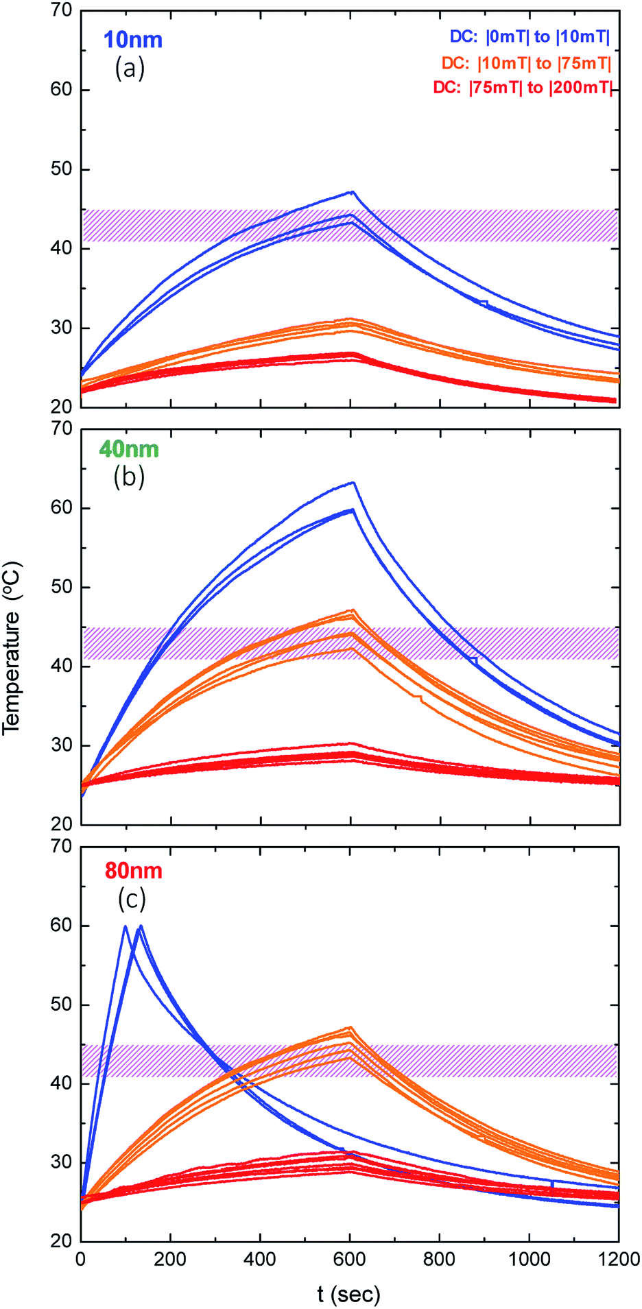Fig. 5 Hyperthermia curves under the AC magnetic field 70 mT/375 kHz and variable constant field magnitude from 0 mT to 200 mT. The hyperthermia window 41–45 °C is depicted with the shaded area. The first part of the curve corresponds to the heating stage (600, 600 and 170 s for 10, 40 and 80 nm respectively). Thereafter, the cooling curve is recorded for ambient time (i.e. ≥ 600 s), resulting in a characteristic exponential decay form, till the sample returns to its initial temperature. Blue, orange and red curves correspond to the constant magnetic field magnitude varying from 0 to 10 mT, 10 to 75 mT and 75 to 200 mT respectively.

Fig. 6 depicts the heating efficiency dependency, in terms of SLP index, on the constant (DC) field magnitude. The horizontal colour scale bar depicts the constant magnetic field magnitude. We observe that inside the FFR region, where the magnitude of the constant magnetic field is almost zero, nanoparticles reach their maximal heating efficiency, due to the absence of the constant magnetic field. Moreover, the SLP value increases with the AC applied magnetic field inside the FFR region. More specifically, the SLP values vary from 25 to 85 W g⁻¹, 82 to 315 W g⁻¹ and 135 to 555 W g⁻¹ with an AC magnetic field amplitude of 40 to 70 mT, for the 10, 40 and 80 MNPs, respectively. It is interesting to note that these results match well with those of the AC magnetic field alone (Fig. 3), which means that the constant magnetic field does not affect the SLP values inside the FFR region. Due to the absence of the constant magnetic field the magnetization of the MNPs freely rotates with the alternating field, when residing within the FFR, giving a sinusoidal magnetization time response that triggers the heating mechanisms irrespective of the nanoparticle size (relaxation or hysteresis losses).

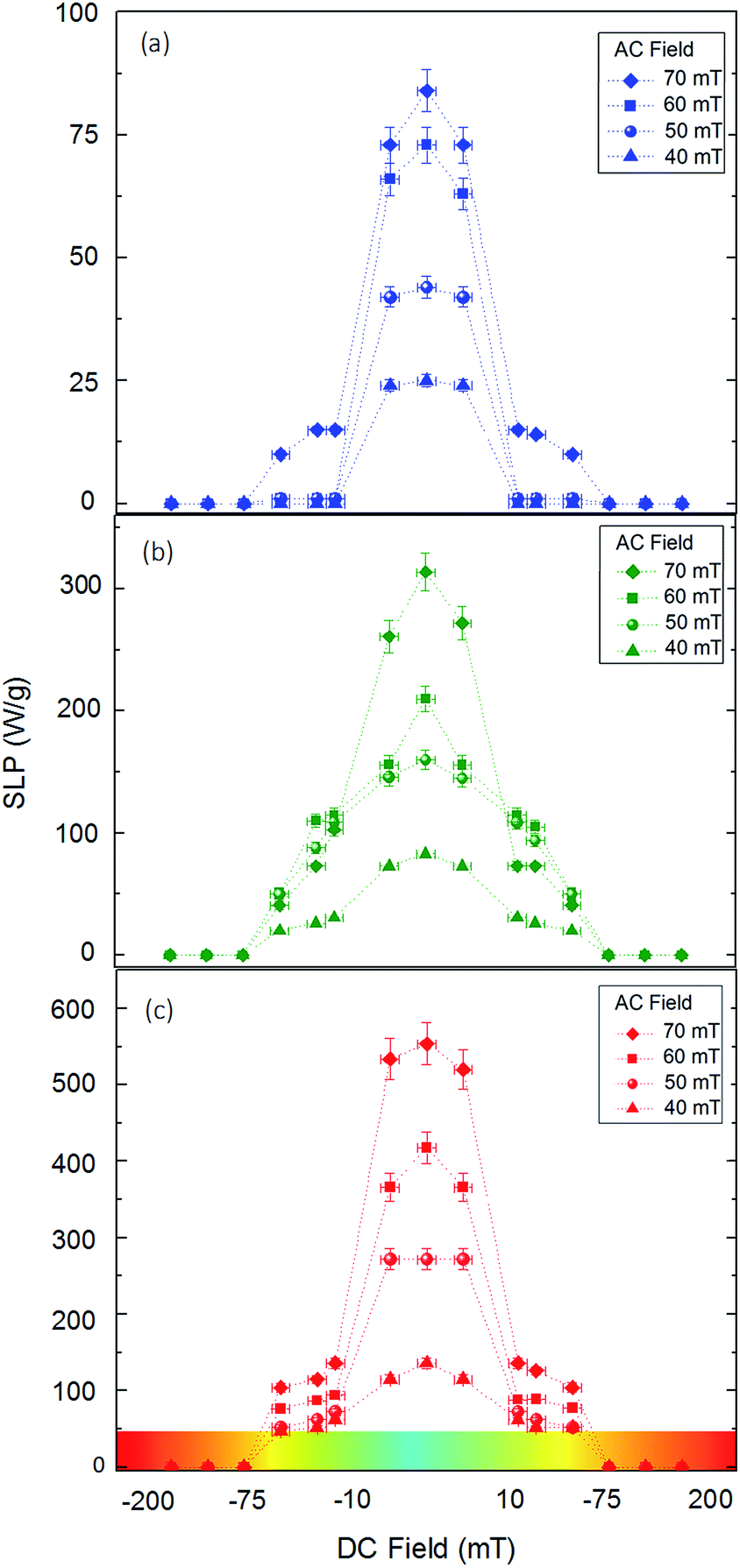Fig. 6 SLP values as a function of the constant magnetic field with respect to the applied alternating magnetic field varying from 40, 50, 60 to 70 mT (375 kHz) with diameters (a) 10 (b) 40 and (c) 80 nm using the setup with the two rectangular magnets. The colour scale bar depicts the strength of the constant magnetic field.

In contrast, if we increase the magnitude of the constant magnetic field, the SLP value decreases rapidly. More specifically, by increasing the magnitude of the constant magnetic field up to 10 mT, it can be observed that the heating efficiency decreases by 60 to 80% depending of the size of MNPs. If we increase more the strength of the constant magnetic field, approximately between 75 and 200 mT, the nanoparticles enter the SR region. The presence of a strong constant magnetic field aligns the MNP magnetizations with its direction with the AC magnetic field causing only minor oscillations in the magnetization response and thus magnetic heating mechanisms are cancelled out. This situation leads to a great reduction in the SLP value by about 100% for all size cases under investigation. Thus, a constant magnetic field of 75 mT seems sufficient to completely saturate the magnetization of the specific MNPs that we used in this study and suppress their heating efficiency in an external AC field.

Such results are in good agreement with previous studies,^16–18 where under the influence of a constant magnetic field, up to 25 mT, MNPs were demonstrated to be saturated outside the FFR leading to focused and selective heating within the FFR, thus making them ideal agents for theranostic applications.

Nowadays, in potential theranostic platforms, magnetic nanoparticles may also be implemented to provide monitoring of diseased regions. Thus, if adequately functionalized, magnetic nanoparticles may provide magnetic hyperthermia while simultaneously acting as an MRI contrast agent.

Even for a relatively small constant magnetic field magnitude (10 mT), an almost 70% decrease occurred in the SLP values for all the MNP systems studied, while for higher constant field magnitude values (occurring as we approach the magnet's edges), where the constant magnetic field is equal to 200 mT, the SLP gradually tends to zero. By using a constant magnetic field, we observed that MNP heating response changed and selectively focused into the FFR, where the SLP values appear unaffected. In contrast, outside the FFR region the MNPs experience competing torques acting on them when the direction of the alternating field is opposite to the constant magnetic field, slowing down particle alignment, but also the action of additive torques speeds up the alignment process, when the static and alternating fields are in the same direction. For the case of the ferromagnetic 40 and 80 nm MNPs, this induces an asymmetry to the shape of the hysteresis loop that results in a decrease in its area.^60,61 For the case of the SPM 10 nm MNPs, the presence of the constant magnetic field changes substantially the magnetization relaxation time and dynamics leading to reduced MNP heating efficiency.^62,63

Discussion

To better understand the strong influence of the constant magnetic field on the SLP index, we mapped the SLP spatial distribution by taking individual SLP measurements following eqn (1) in specific positions, defined at the working space illustrated in Fig. 7.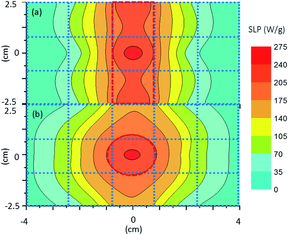

Fig. 7 Spatial heating distribution of experimental SLP values with the alternating magnetic field at 50 mT and frequency 375 kHz and using constant magnetic fields of (a) two rectangular parallelepiped and (b) four cubic permanent NdFeB magnets. The sample under study was made with 80 nm MNPs. The colour scale bar depicts the heating efficiency. The blue colour refers to the minimum value (0 W g⁻¹) and the red to the maximum value (275 W g⁻¹) of SLP.

A contour plot of SLP values that resulted after the experimental measurements was obtained inside the workspace at the 15 spots according to the geometry of the FFR. The SLP values increased in the range from minimum to maximum with the blue-red colour, respectively, as a function of the distance from the permanent magnets. The range of experimental data varied from 0 to 275 W g⁻¹ while the applied AC field was kept constant at 50 mT and 375 kHz. Experimental results were taken for the biggest size of nanoparticles (80 nm) using the two different constant magnetic configurations. The contour plot shows clearly that, for both permanent magnet setups, the MNP heating efficiency can be spatially focused inside the FFR region. The MNPs appear to be fully saturated outside the FFR region, due to the presence of the constant magnetic field, leading to a minimization of their heating efficiency while inside the FFR region maximum heating efficiency was observed in the absence of the constant magnetic field. Even in the presence of relatively small (from 10 to 75 mT) constant magnetic fields, SLP values were approximately 70% decreased while stronger (above 75 mT) constant magnetic fields succeeded in attenuating the MNP heating efficiency.

A clinical application of such a magnetically driven treatment typically starts with the direct injection of the corresponding carriers i.e. the magnetic nanoparticles straight into the malignant region. Generally, when magnetic nanoparticles are subjected to an inhomogeneous magnetic field, they tend to move to areas of a higher magnetic field due to field gradients. However, nanoparticles in vivo are internalized by cells by endocytosis and reside in membrane-bound vesicles, known as endosomes, right after endocytosis.^64,65 Cell magnetophoresis, a crucial issue for the clinical practice translation (analogous to cell electrophoresis), may occur⁶⁶ with a very small average velocity of cells (3 μm s⁻¹) in a gradient of 18.5 mT mm⁻¹, which is however much larger than the gradient field in our experiments (5 mT mm⁻¹).

By implementing the two different setups of magnets, the shape of the targeted hyperthermia region may vary accordingly, following the constant field strength variation as shown in Fig. 4 with a limited “targeted” area region e.g. of 1.5 × 5 cm² (Fig. 7). The constant magnetic field in the FFR region is so weak that after the injection the nanoparticles remain practically stable at their positions, delivering their maximum heat cargo. Such an application was tested in vivo by Tasci et al.⁶⁷ where 10 nm iron magnetic nanoparticles were (a) injected and found to be homogenously distributed in adult mice tails (mimicking bone and skin muscle tissues) and (b) exposed to an AC field of 7.6 kA m⁻¹, 80 kHz in combination with three different static fields for 25 min. Eventually, regional burning was tuned by adequately varying the magnetic field strength.

Consequently, such an application scheme, provided that adequate tuning is achieved with respect to certain tumour morphological features, promotes spatially focused MPH, without compromising the heating efficiency of MNPs, but sparing the surrounding healthy tissues. Since the DC field application is a prerequisite for image formation in MPI, such an approach has potential theranostics applications.

Conclusions

In this study, we propose two alternative experimental setups that spatially focused magnetic particle hyperthermia with the concurrent application of a constant magnetic field generated using two different configurations of permanent NdFeB magnets. These setups generate an FFR which can be manipulated in shape and size according to the magnetic field distributions. We investigated the effect of the constant magnetic field magnitude on the SLP and then evaluated the feasibility of controlling the SLP values using the FFR in various combinations of alternating and constant magnetic fields. Our results demonstrate that it is possible to spatially control the temperature rise in magnetic particle hyperthermia using the proposed approach. Since the energy dissipation and temperature rise in magnetic particle hyperthermia largely depend on the size of MNPs we examined three distinctly different magnetic behaviour cases with respect to iron oxide MNP diameters ranging from superparamagnetism, for a diameter of 10 nm, to multi-domain ferromagnetism, for a diameter of 80 nm.

Conflicts of interest

There are no conflicts to declare.

Acknowledgements

This project has been supported by the General Secretariat of Research and Technology (GSRT) and the Hellenic Foundation for Research and Innovation (HFRI). This research was also co-financed by Greece and the European Union (European Social Fund – ESF) through the Operational Programme (Human Resources Development, Education and Lifelong Learning) in the context of the project “Strengthening Human Resources Research Potential via Doctorate Research” (MIS-5000432), implemented by the State Scholarships Foundation (IKY).

Notes and references

1. A. Konecny, J. Covarrubias and H. Wang, Magnetic Nanomaterials, 2017, pp. 25–58.
2. A. Curcio, A. K. A. Silva, S. Cabana, A. Espinosa, B. Baptiste, N. Menguy, C. Wilhelm and A. A. Hassan, Theranostics, 2019, 9, 1288.
3. S. Moise, J. M. Byrne, A. J. El Haj and N. D. Telling, Nanoscale, 2018, 10, 20519–20525.
4. E. A. Périgo, G. Hemery, O. Sandre, D. Ortega, E. Garaio, F. Plazaola and F. J. Teran, Appl. Phys. Rev., 2015, 2, 041302.
5. K. Kaczmarek, T. Hornowski, I. Antal, M. Timko and A. Józefczak, J. Magn. Magn. Mater., 2019, 474, 400–405.
6. A. S. Jordan, R. Scholz, P. Wust, H. Fahling, J. Krause, W. Wlodarczyk, B. Sander, T. Vogl and R. Felix, Int. J. Hyperthermia, 1997, 13, 587–605.
7. A. P. Khandhar, R. M. Ferguson, J. A. Simon and K. M. Krishnan, J. Appl. Phys., 2012, 111, 07B3061.
8. M. Angelakeris, Biochim. Biophys. Acta, Gen. Subj., 2017, 1861, 1642–1651.
9. W. Wu, C. Jiang and V. A. L. Roy, Nanoscale, 2016, 8, 19421–19474.
10. H. A. Albarqi, L. H. Wong, C. Schumann, F. Y. Sabei, T. Korzun, X. Li, M. N. Hansen, P. Dhagat, A. S. Moses, O. Taratula and O. Taratula, ACS Nano, 2019, 13, 6383–6395.
11. K. Maier-Hauff, R. Rothe, R. Scholz, U. Gneveckow, P. Wust, B. Thiesen, A. Feussner, A. Deimling, N. Waldoefner, R. Felix and A. Jordan, J. Neurooncol., 2007, 81, 53–60.
12. K. Maier-Hauff, F. Ulrich, D. Nestler, H. Niehoff, P. Wust, B. Thiesen, H. Orawa, V. Budach and A. Jordan, J. Neurooncol., 2011, 103, 317–324.
13. B. Thiesen and A. Jordan, Int. J. Hyperthermia, 2008, 24, 467–474.
14. O. Grauer, M. Jaber, K. Hess, M. Weckesser, W. Schwindt, S. Maring, J. Wolfer and W. Stummer, J. Neuro-Oncol., 2019, 141, 83–94.
15. M. Johannsen, U. Gneveckow, L. Eckelt, A. Feussner, N. WaldÖFner, R. Scholz, S. Deger, P. Wust, S. A. Loening and A. Jordan, Int. J. Hyperthermia, 2005, 21, 637–647.
16. M. Johannsen, U. Gneveckow, B. Thiesen, K. Taymoorian, C. H. Cho, N. Waldofner, R. Scholz, A. Jordan, S. A. Loening and P. Wust, Eur. Urol., 2007, 52, 1653–1662.
17. M. H. Pablico-Lansigan, S. F. Situ and A. C. S. Samia, Nanoscale, 2013, 10, 4040–4055.
18. L. C. Wu, Y. Zhang, G. Steinberg, H. Qu, S. Huang, M. Cheng, T. Bliss, F. Du, J. Rao, G. Song, L. Pisani, T. Doyle, S. Conolly, K. Krishnan, G. Grant and M. Wintermark, Am. J. Neuroradiol., 2019, 40, 206–212.
19. S. Sánchez-Cabezas, R. Montes-Robles, J. Gallo, F. Sancenón and R. Martínez-Máñez, Dalton Trans., 2019, 48, 3883–3892.
20. L. Wöckel, J. Wells, O. Kosch, S. Lyerc, C. Alexiou, C. Grüttnerd, F. Wiekhorst and S. Dutz, J. Magn. Magn. Mater., 2019, 471, 1–7.
21. J. Weizenecker, B. Gleich, J. Rahmer, H. Dahnke and J. Borgert, Phys. Med. Biol., 2009, 54, L1–L10.
22. B. Mehdaoui, J. Carreya, M. Stadler, A. Cornejo, C. Nayral, F. Delpech, B. Chaudret and M. Respaud, Appl. Phys. Lett., 2012, 100, 052403.
23. L. M. Bauer, S. F. Situ, M. A. Griswold and A. C. S. Samia, Nanoscale, 2016, 8, 12162–12169.
24. L. Chun, Nat. Mater., 2014, 13, 110.
25. D. Hensley, Z. W. Tay, R. Dhavalikar, B. Zheng, P. Goodwill, C. Rinaldi and S. Conolly, Phys. Med. Biol., 2017, 62, 3483.
26. D. Hensley, Z. W. Tay, R. Dhavalikar, P. Goodwill, B. Zheng, C. Rinaldi and S. Conolly, Int. Soc. Opt. Photon., 2017, 10066, 1006603.
27. K. Murase, H. Takata, Y. Takeuchi and S. Saito, Phys. Med., 2013, 29, 624–630.
28. K. Murase, Open J. Appl. Sci., 2016, 6(12), 839.
29. R. Dhavalikar and C. Rinaldi, J. Magn. Magn. Mater., 2016, 419, 267–273.
30. B. Mehdaoui, J. Carrey, M. Stadler, A. Cornejo, C. Nayral, F. Delpech and M. Respaud, Appl. Phys. Lett., 2012, 100, 052403.
31. J.-P. Fortin, C. Wilhelm, J. Servais, C. Ménager, J.-C. Bacri and F. Gazeau, J. Am. Chem. Soc., 2007, 129, 2628–2635.
32. P. De la Presa, Y. Luengo, M. Multigner, R. Costo, M. P Morales, G. Rivero and A. Hernando, J. Phys. Chem. C, 2012, 116, 25602–25610.
33. X. L. Liu, H. M. Fan, J. B. Yi, Y. Yang, E. S. G. Choo, J. M. Xue, D. D. Fan and J. Ding, J. Mater. Chem., 2012, 22, 8235–8244.
34. A. Jordan, T. Rheinländer, N. Waldöfner and R. Scholz, J. Nanopart. Res., 2003, 5, 597–600.
35. Z. Nemati, J. Alonso, I. Rodrigo, R. Das, E. Garaio, J. Á. García, I. Orue, M. H. Phan and H. Srikanth, J. Phys. Chem. C, 2018, 122, 2367–2381.
36. Y. Lv, Y. Yang, J. Fanga, H. Zhanga, E. Penga, X. Liuac, W. Xiaoa and J. Ding, RSC Adv., 2015, 5, 76764–76771.
37. A. Hervault and N. T. K. Thanh, Nanoscale, 2014, 6, 11553–11573.
38. J. Carreya, B. Mehdaoui and M. Respaud, J. Appl. Phys., 2011, 109, 083921.
39. D. Shi, M. E. Sadat, A. W. Dunn and D. B. Mast, Nanoscale, 2015, 7, 8209–8232.
40. E. Myrovali, N. Maniotis, A. Makridis, A. Terzopoulou, V. Ntomprougkidis, K. Simeonidis, D. Sakellari, O. Kalogirou, T. Samaras, R. Salikhov, M. Spasova, M. Farle, U. Wiedwald and M. Angelakeris, Sci. Rep., 2016, 6, 37934.
41. A. Makridis, S. Curto, G. C. van Rhoon, T. Samaras and M. Angelakeris, J. Phys. D: Appl. Phys., 2019, 52, 255001.
42. https://www.supermagnete.gr .
43. Comsol Multiphysics Tutorial, AC/DC Model, version 3.5a.
44. A. Kovetz, The Principles of Electromagnetic Theory, Cambridge University Press, 1990.
45. J. Jin, The Finite Element Method in Electromagnetics, 2nd edn, Wiley-IEEE Press, May 2002.
46. D. Brown, B. M. Ma and Z. Chen, J. Magn. Magn. Mater., 2002, 248, 432–440.
47. L. Gutierrez, M. Moros, E. Mazario, S. de Bernardo, J. M. de la Fuente, M. del Puerto Morales and G. Salas, Nanotechnology, 2019, 30, 112001.
48. M.-H. Phan, J. Alonso, H. Khurshid, P. Lampen-Kelley, S. Chandra, K. Stojak Repa, Z. Nemati, R. Das, Ó. Iglesias and H. Srikanth, Nanomaterials, 2016, 6, 221.
49. K. D. Bakoglidis, K. Simeonidis, D. Sakellari, G. Stefanou and M. Angelakeris, IEEE Trans. Magn., 2012, 48, 1320–1323.
50. A. G. Roca, R. Costo, A. F. Rebolledo, S. Veintemillas-Verdaguer, P. Tartaj, T. González-Carreño, M. P. Morales and C. J. Serna, J. Phys. D. Appl. Phys., 2009, 42, 224002.
51. K. J. Klabunde, Nanoscale Material in Chemistry, Wiley-Interscience, New York, 2001.
52. R. E. Rosensweig, J. Magn. Magn. Mater., 2002, 252, 370–374.
53. S. Tong, C. A. Quinto, L. Zhang, P. Mohindra and G. Bao, ACS Nano, 2017, 11, 6808–6816.
54. Z. Nemati, R. Das, J. Alonso, E. Clements, M. H. Phan and H. Srikanth, J. Electron. Mater., 2017, 46, 3764–3769.
55. J. Carrey, B. Mehdaoui and M. Respaud, J. Appl. Phys., 2011, 109, 083921.
56. N. Maniotis, A. Nazlidis, E. Myrovali, A. Makridis, M. Angelakeris and T. Samaras, J. Appl. Phys., 2019, 125, 103903.
57. M. Angelakeris, Biochim. Biophys. Acta Gen. Subj., 2017, 1861, 1642–1651.
58. K. M. Krishnan, IEEE Trans. Magn., 2010, 46, 2523–2558.
59. Y. S. Kwon, K. Sim, T. Seo, J. K. Lee, Y. Kwon and T. J. Yoon, RSC Adv., 2016, 6, 107298–107304.
60. R. Dhavalikar and C. Rinaldi, J. Magn. Magn. Mater., 2016, 419, 267–273.
61. P. M. Déjardin, Yu. P. Kalmykov, B. E. Kashevsky, H. El Mrabti, I. S. Poperechny, Yu. L. Raikhe and S. V. Titov, J. Appl. Phys., 2010, 107, 073914.
62. S. , V. T. Halim El Mrabti, P.-M. Déjardin and Y. P. Kalmykov, J. Appl. Phys., 2011, 110, 023901.
63. K. Murase, H. Takata, Y. Takeuchi and S. Saito, Phys. Med., 2013, 29, 624–630.
64. E. Teeman, C. Shasha, J. E. Evans and K. M. Krishnan, Nanoscale, 2019, 11, 7771–7780.
65. G. Sahay, D. Y. Alakhova and A. V. Kabanov, J. Controlled Release, 2010, 145, 182–195.
66. C. Wilhelm, F. Gazeau and J. C. Bacri, Eur. Biophys. J., 2002, 31, 118–125.
67. T. O. Tasci, I. Vargel, A. Arat, E. Guzel, P. Korkusuz and E. Atalar, Med. Phys., 2009, 36, 1906–1912.

---