ProteoViz: a tool for the analysis and interactive visualization of phosphoproteomics data

Abstract

Quantitative proteomics generates large datasets with increasing depth and quantitative information. With the advance of mass spectrometry and increasingly larger data sets, streamlined methodologies and tools for analysis and visualization of phosphoproteomics are needed both at the protein and modified peptide levels. To assist in addressing this need, we developed ProteoViz, which includes a set of R scripts that perform normalization and differential expression analysis of both the proteins and enriched phosphorylated peptides, and identify sequence motifs, kinases, and gene set enrichment pathways. The tool generates interactive visualization plots that allow users to interact with the phosphoproteomics results and quickly identify proteins and phosphorylated peptides of interest for their biological study. The tool also links significant phosphosites with sequence motifs and pathways that will help explain the experimental conditions and guide future experiments. Here, we present the workflow and demonstrate its functionality by analyzing a phosphoproteomic data set from two lymphoma cell lines treated with kinase inhibitors. The scripts and data are freely available at https://github.com/ByrumLab/ProteoViz and via the ProteomeXchange with identifier PXD015606.

---

Introduction

The field of proteomics has developed significantly in recent years,^1,2 allowing for an unprecedented view of the proteome and post-translationally modified proteome. Advances in sample preparation,^3–5 instrumentation,⁶ and data acquisition^7–9 have culminated in increasingly large biological datasets containing precise measurements of thousands of proteins and modifications from dozens of samples. The ability to increase sequencing depth for quantitation has led to a greater number of differentially abundant features in a given experiment, which in turn provides a more comprehensive view of how biological perturbations affect the proteome, modified proteome, and ultimately phenotype.

Protein phosphorylation is a ubiquitous post-translational modification (PTM) affecting nearly every biological pathway.¹⁰ Signal transduction cascades, metabolic pathways, regulation of DNA replication, repair, and gene expression, are all regulated in part by dynamic phosphorylation. With the advancement in mass spectrometry technology, it is now feasible to quantify more than 10 000 phosphorylation sites in a single study. The increase of sequencing depth requires new tools to analyze all of the peptides. Therefore, we developed ProteoViz as a tool for the analysis and visualization of proteins and phosphorylated peptides. ProteoViz starts with the MaxQuant database search results, a sample metadata file, and a contrast matrix file as inputs and performs limma differential expression at both the protein and phosphopeptide levels, motif sequence analysis, and pathway analysis. The results are displayed in an interactive dashboard to allow investigators to quickly interpret the results.

The dashboard is powered by Shiny, an R package, which enables the construction of interactive HTML documents using only R code. Since bioinformatics is routinely performed using the R programming language, the output of a bioinformatics pipeline can be passed into an interactive dashboard without having to learn a new programming language. In turn, the dashboards allow the end user to access and efficiently process the data from a web browser without having to learn R.

Here, we describe the components of ProteoViz and demonstrate their use on a phosphoproteomic study, in which two diffuse large B-cell lymphoma cell lines were treated with one of two inhibitors of a cell cycle kinase (iCCK1 or iCCK2).

Methods

Cell culturing

The VAL cell line was previously obtained from Dr Staudt (NCI) and the SUDHL5 cell line was purchased from the American Type Culture Collection (CRL-2958). Both diffuse large B-cell lymphoma cell lines were cultured in Roswell Park Memorial Institute (RPMI) supplemented with 10% fetal bovine serum (FBS) and 1% penicillin/streptomycin. Cell lines were tested for mycoplasma every 6 months using the MycoAlert Plus detection kit (Lonza) with the MycoAlert Assay control set and authenticated by the University of Arizona Genetics Core (Tucson, AZ) using the PowerPlex 16 System (Promega), which consists of forensic-style 15 autosomal short tandem repeat (STR) loci, including 13 combined DNA index system (CODIS) DNA markers (nine of the standard loci collected by ATCC), amelogenin, and a mouse-specific locus, every 12 months.

Sample preparation

Cells were grown to confluence at >90% viability before setting in 25 mL cell culture flask at a density of 250 000 cells per mL and equilibrated overnight. Cells were then treated with vehicle (0.1% DMSO), iCCK1 (inhibitor of cell cycle kinase 1), or iCCK2 and incubated for 96 hours at 37 °C, 5% CO₂. The final concentrations for iCCK1 treatment were 240 nM or 80 nM, VAL or SUDHL5, respectively. For iCCK2 treatment, both VAL and SUDHL5 received 470 nM. Three independent treatments were performed and cell pellets from each were harvested by centrifugation (400g, 5 min) and washed three times with 1× PBS (pH = 7.4) before flash freezing in liquid nitrogen. Cell pellets were stored at −80 °C before the triplicate samples were submitted for proteomic analysis.

Mass spectrometry

Purified proteins were reduced, alkylated, and digested using filter-aided sample preparation [Nat. Methods, 2009, 6, 359–362]. Tryptic peptides were labeled using a tandem mass tag (TMT) 10-plex isobaric label reagent set (Thermo) and enriched using a High-Select TiO₂ phosphopeptide enrichment kit (Thermo) following the manufacturer's instructions with the following slight modifications. The centrifugation speed was reduced for sample loading from 1000g to 700g, and an additional phosphopeptide elution step was performed after the recommended elution steps, using 50 μl of 1 : 1 H20 : ACN with 10 mM NH₄OH. Both enriched and un-enriched labeled peptides were separated into 36 fractions on a 100 × 1.0 mm Acquity BEH C18 column (Waters) using an UltiMate 3000 UHPLC system (Thermo) with a 40 min gradient from 99 : 1 to 60 : 40 buffer A : B ratio under basic (pH 10) conditions, and then consolidated into 12 super-fractions. Buffer A contains 0.5% acetonitrile and 10 mM ammonium hydroxide. Buffer B contains 10 mM ammonium hydroxide in acetonitrile. Each super-fraction was then further separated by reverse phase XSelect CSH C18 2.5 μm resin (Waters) on an in-line 150 × 0.075 mm column using an UltiMate 3000 RSLCnano system (Thermo). Peptides were eluted using a 60 min gradient from 97 : 3 to 60 : 40 buffer A : B ratio. Here, buffer A contains 0.1% formic acid and 0.5% acetonitrile and buffer B contains 0.1% formic acid and 99.9% acetonitrile. Eluted peptides were ionized by electrospray (2.15 kV) followed by mass spectrometric analysis on an Orbitrap Fusion Lumos mass spectrometer (Thermo) using multi-notch MS³ parameters. MS data were acquired using the FTMS analyzer in top-speed profile mode at a resolution of 120 000 over a range of 375 to 1500 m/z. Following CID activation with normalized collision energy of 35.0, MS/MS data were acquired using the ion trap analyzer in centroid mode and normal mass range. Using synchronous precursor selection, up to 10 MS/MS precursors were selected for HCD activation with normalized collision energy of 65.0, followed by acquisition of MS³ reporter ion data using the FTMS analyzer in profile mode at a resolution of 50 000 over a range of 100–500 m/z. A sample preparation workflow is described in Fig. 1A.

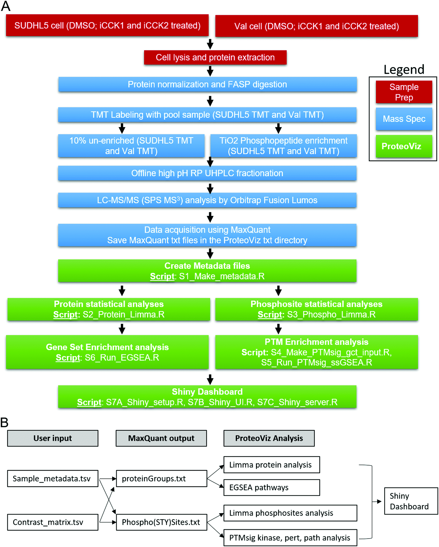Fig. 1 Overview of ProteoViz workflow. (A) The workflow from sample preparation, the mass spectrometric methods, and the data analysis using ProteoViz. Two cell lines were treated with and without iCCK1 or iCCK2 kinase inhibitors, cell lysates were FASP digested and labeled with tandem mass tags. Each sample was split with 10% of the sample prepared for total protein analysis and 90% of the sample underwent a TiO₂ Phosphopeptide enrichment. The samples were fractionated using offline high pH reverse-phase UHPLC fractionation, analyzed by Oribitrap Fusion Lumos, and followed by a MaxQuant database search. The MaxQuant output files were then imported into ProteoViz for protein and phosphosite statistical analysis and displayed in an interactive Shiny dashboard. (B) The user supplied input files connected to the MaxQuant output files and how each connect to the ProteoViz analytical workflow.

Database search

Proteins were identified and reporter ions quantified by searching the UniprotKB Homo sapiens database (April 2019) using MaxQuant (version 1.6.5.0, Max Planck Institute) with a parent ion tolerance of 3 ppm, a fragment ion tolerance of 0.5 Da, a reporter ion tolerance of 0.001 Da, trypsin/P enzyme with 2 missed cleavages, variable modifications including oxidation on M, acetyl on protein N-term, and phosphorylation on STY, and fixed modification of carbamidomethyl on C. Protein identifications were accepted if they could be established with less than 1.0% false discovery. Proteins identified only by modified peptides were removed. Protein probabilities were assigned by the Protein Prophet algorithm [Anal. Chem., 2003, 75, 4646–4658].

TMT MS³ reporter ion intensity values were analyzed for changes in total protein using the un-enriched lysate sample. Phospho(STY) modifications were identified using the samples enriched for phosphorylated peptides. The enriched and un-enriched samples were multiplexed using two TMT10-plex batches, one for the enriched and one for the un-enriched samples.

Data analysis using ProteoViz

In order to use ProteoViz a few input files are required in the R project folder. The MaxQuant database result files should be saved in a “txt” folder and must include the “ProteinGroups.txt” and the “Phospho(STY)Sites.txt” files (Tables S1 and S2, ESI†). A “database” folder should include the “ptm.sig.db.all.flanking.human.v1.8.1.gmt” file for the PTMSig/ssGSEA analysis, and the “Human_entrez_map.tsv.gz” and “msigdb.v6.2.entrez.gmt” files for the Ensemble of Gene Set Enrichment Analyses (EGSEA) analysis. All R scripts are saved in a “src” folder. A Sample_metadata.tsv and a contrast_matrix.tsv file should be created and saved in the R project folder. The Sample_metadata.tsv file includes the column names for the TMT MS3 reporter ion corrected intensities from the MaxQuant output, the sample names that match the TMT reporter ion channels, and the group and replicate information (Table 1). The names listed in the Sample_metadata.tsv file is then translated into the visualization plots. The contrast_matrix.tsv file includes the sample group comparisons that will be used in the limma statistical analysis (Table 2). Once all the files are in the appropriate folders, each of the R scripts are run in consecutive order.

Table 1 Sample metadata file for specifying sample names and statistics groups. The sample column matches the column names of the MaxQuant search output. The enrichment, batch, and pool columns denote phosphoenrichment status, batch number, and pooled reference status. Each sample is given a unique name in the Sample_name column, and designated to a model group for use in statistics testing

Sample	Enrichment	Batch	Replicate	Pool	Sample_name	Model_group
Reporter_intensity_corrected_4_TMT1	Lysate	0	1		Cell1_DMSO_1	Cell1_DMSO
Reporter_intensity_corrected_5_TMT1	Lysate	0	2		Cell1_DMSO_2	Cell1_DMSO
Reporter_intensity_corrected_6_TMT1	Lysate	0	3		Cell1_DMSO_3	Cell1_DMSO
Reporter_intensity_corrected_1_TMT1	Lysate	0	1		Cell1_inhibitor1_1	Cell1_inhibitor1
Reporter_intensity_corrected_2_TMT1	Lysate	0	2		Cell1_inhibitor1_2	Cell1_inhibitor1
Reporter_intensity_corrected_3_TMT1	Lysate	0	3		Cell1_inhibitor1_3	Cell1_inhibitor1
Reporter_intensity_corrected_7_TMT1	Lysate	0	1		Cell1_inhibitor2_1	Cell1_inhibitor2
Reporter_intensity_corrected_8_TMT1	Lysate	0	2		Cell1_inhibitor2_2	Cell1_inhibitor2
Reporter_intensity_corrected_9_TMT1	Lysate	0	3		Cell1_inhibitor2_3	Cell1_inhibitor2
Reporter_intensity_corrected_10_TMT1	Lysate	0		POOL
Reporter_intensity_corrected_4_TMT2	Lysate	1	1		Cell2_DMSO_1	Cell2_DMSO
Reporter_intensity_corrected_5_TMT2	Lysate	1	2		Cell2_DMSO_2	Cell2_DMSO
Reporter_intensity_corrected_6_TMT2	Lysate	1	3		Cell2_DMSO_3	Cell2_DMSO
Reporter_intensity_corrected_1_TMT2	Lysate	1	1		Cell2_inhibitor1_1	Cell2_inhibitor1
Reporter_intensity_corrected_8_TMT2	Lysate	1	2		Cell2_inhibitor1_2	Cell2_inhibitor1
Reporter_intensity_corrected_3_TMT2	Lysate	1	3		Cell2_inhibitor1_3	Cell2_inhibitor1
Reporter_intensity_corrected_7_TMT2	Lysate	1	1		Cell2_inhibitor2_1	Cell2_inhibitor2
Reporter_intensity_corrected_2_TMT2	Lysate	1	2		Cell2_inhibitor2_2	Cell2_inhibitor2
Reporter_intensity_corrected_9_TMT2	Lysate	1	3		Cell2_inhibitor2_3	Cell2_inhibitor2
Reporter_intensity_corrected_10_TMT2	Lysate	1		POOL
Reporter_intensity_corrected_4_TMT1phos	Phos	0	1		Cell1_DMSO_1	Cell1_DMSO
Reporter_intensity_corrected_5_TMT1phos	Phos	0	2		Cell1_DMSO_2	Cell1_DMSO
Reporter_intensity_corrected_6_TMT1phos	Phos	0	3		Cell1_DMSO_3	Cell1_DMSO
Reporter_intensity_corrected_1_TMT1phos	Phos	0	1		Cell1_inhibitor1_1	Cell1_inhibitor1
Reporter_intensity_corrected_2_TMT1phos	Phos	0	2		Cell1_inhibitor1_2	Cell1_inhibitor1
Reporter_intensity_corrected_3_TMT1phos	Phos	0	3		Cell1_inhibitor1_3	Cell1_inhibitor1
Reporter_intensity_corrected_7_TMT1phos	Phos	0	1		Cell1_inhibitor2_1	Cell1_inhibitor2
Reporter_intensity_corrected_8_TMT1phos	Phos	0	2		Cell1_inhibitor2_2	Cell1_inhibitor2
Reporter_intensity_corrected_9_TMT1phos	Phos	0	3		Cell1_inhibitor2_3	Cell1_inhibitor2
Reporter_intensity_corrected_10_TMT1phos	Phos	0		POOL
Reporter_intensity_corrected_4_TMT2phos	Phos	1	1		Cell2_DMSO_1	Cell2_DMSO
Reporter_intensity_corrected_5_TMT2phos	Phos	1	2		Cell2_DMSO_2	Cell2_DMSO
Reporter_intensity_corrected_6_TMT2phos	Phos	1	3		Cell2_DMSO_3	Cell2_DMSO
Reporter_intensity_corrected_1_TMT2phos	Phos	1	1		Cell2_inhibitor1_1	Cell2_inhibitor1
Reporter_intensity_corrected_8_TMT2phos	Phos	1	2		Cell2_inhibitor1_2	Cell2_inhibitor1
Reporter_intensity_corrected_3_TMT2phos	Phos	1	3		Cell2_inhibitor1_3	Cell2_inhibitor1
Reporter_intensity_corrected_7_TMT2phos	Phos	1	1		Cell2_inhibitor2_1	Cell2_inhibitor2
Reporter_intensity_corrected_2_TMT2phos	Phos	1	2		Cell2_inhibitor2_2	Cell2_inhibitor2
Reporter_intensity_corrected_9_TMT2phos	Phos	1	3		Cell2_inhibitor2_3	Cell2_inhibitor2
Reporter_intensity_corrected_10_TMT2phos	Phos	1		POOL

---

Table 2 Contrast matrix file setup. The contrast matrix file details the model groups, which are compared for each statistical test. The names follow the contrast nomenclature from the Limma package

Contrast_name

Cell2_DMSO – Cell1_DMSO

Cell1_inhibitor1 – Cell1_DMSO

Cell1_inhibitor2 – Cell1_DMSO

Cell2_inhibitor1 – Cell2_DMSO

Cell2_inhibitor2 – Cell2_DMSO

---

The output files are saved in a “data” folder and includes the protein_limma_input.tsv, protein_limma_output.tsv, protein_metadata.tsv, phospho_limma_input.tsv, phospho_limma_output.tsv, phospho_metadat.tsv, protein_summarized_data.tsv, and the phospho_summarized_data.tsv files. The results from the PTM signatures database (PTMsig)¹¹ and EGSEA¹² are saved in separate folders in the “data” folder. These files are used to generate the interactive plots in the Shiny dashboard. The sample preparation, mass spectrometric, and ProteoViz workflow is shown in Fig. 1. The input and output files for each ProteoViz script are listed in Table 3.

Table 3 ProteoViz analysis scripts input and output files. Each script requires certain input files and these are listed with the directory location. The output files from the scripts become the input file for the following script. All of the output files are loaded into the Shiny scripts and visualized in an interactive Shiny Dashboard

Function	Script	Input files	Output files
Create metadata	S1_Make_metadata.R	txt/proteinGroups.txt	data/Protein_metadata.tsv
		txt/Phospho(STY)Sites.txt	data/Phospho_metadata.tsv
Protein statistical analysis	S2_Protein_Limma.R	txt/proteinGroups.txt	data/Normalized_proteingroup_intensities.tsv
		Sample_metadata.tsv	data/Protein_limma_input.tsv
		contrast_matrix.tsv	data/Protein_limma_output.tsv
		data/Protein_metadata.tsv	data/Protein_summarized_data.tsv
Phosphosite statistical analysis	S3_Phospho_Limma.R	txt/Phospho(STY)Sites.txt	data/Phospho_limma_input.tsv
		data/Phospho_metadata.tsv	data/Phospho_limma_output.tsv
		Sample_metadata.tsv	data/Phospho_summarized_data.tsv
		contrast_matrix.tsv
		data/Normalized_proteingroup_intensities.tsv
PTMsig: phosphosite kinase, perturbations, and pathway analysis	S4_Make_PTMsig_gct_input.R	txt/Phospho(STY)Sites.txt	data/PTMsig/Phospho_PTMsig_input.gct
		Sample_metadata.tsv
PTMsig: phosphosite kinase, perturbations, and pathway analysis	S5_Run_PTMsig_ssGSEA.R	data/PTMsig/Phospho_PTMsig_input.gct	data/PTMsig/output/output-combined.gct
		databases/ptm.sig.db.all.flanking.human.v1.8.1.gmt	data/PTMsig/output/output-fdr-pvalues.gct
			data/PTMsig/output/output-pvalues.gct
			data/PTMsig/output/output-scores.gct
EGSEA: protein pathway analysis	S6_Run_EGSEA.R	txt/proteinGroups.txt	data/Protein_EGSEA_input.tsv
		Sample_metadata.tsv	data/EGSEA/EGSEA_test_results.tsv
		contrast_matrix.tsv	data/EGSEA/EGSEA_comparison.tsv
		databases/Human_entrez_map.tsv.gz
		databases/msigdb.v6.2.entrez.gmt
Shiny dashboard visualization	S7A_Shiny_setup.R	Sample_metadata.tsv	Plots in the Shiny dashboard
	S7B_Shiny_UI.R	contrast_matrix.tsv
	S7C_Shiny_server.R	data/Protein_limma_input.tsv
		data/Protein_limma_output.tsv
		data/Protein_metadata.tsv
		data/Phospho_metadata.tsv
		data/Phospho_limma_input.tsv
		data/Phospho_limma_output.tsv
		data/PTMsig/output/output-combined.gct
		databases/ptm.sig.db.all.flanking.human.v1.8.1.gmt
		data/PTMsig/Phospho_PTMsig_input.gct
		data/Protein_EGSEA_input.tsv
		databases/msigdb.v6.2.entrez.gmt
		data/EGSEA/EGSEA_test_results.tsv
		data/EGSEA/EGSEA_comparison.tsv

---

Script 1: generate metadata

The ProteoViz includes six R scripts for processing the database search results directly from MaxQuant¹³ proteinGroups.txt and phospho(STY)Sites.txt output files. The ID column in the proteinGroups.txt file is the same as the Protein group ID column in the phospho(STY)Sites.txt file and vice versa, allowing users to link modified peptides to the total protein intensity. The first script, S1_Make_metadata.R, utilizes the tidyverse package to extract the Protein ID, Fasta header, Score, proteinGroups.txt file ID, phospho(STY)Sites.txt ID, protein description, the gene name, and the Uniprot ID into a new “Protein_metadata.txt” file that is used in a downstream analysis step to link the protein information with the phosphorylated peptides.

Script 1 also generates a “Phospho_metatdata.txt” file that contains the protein accession, the position of the PTM within the protein, Fasta header, localization probability, score diff, PEP, Score, the amino acid that is modified, the peptide sequence, the phospho(STY) probabilities within the sequence, charge, phosphoSites.txt ID, peptide id, protein group id, description of the protein, gene name, Uniprot ID, and the flanking sequence. The flanking sequence is the modified amino acid plus/minus 7 amino acids. This information is used in the PTMsig analysis to identify sequence motifs.

Script 2: protein statistical analysis

The second R script, S2_Protein_Limma.R, is used to run statistical analysis of the protein data using the R packages tidyverse and limma.¹⁴ First, the proteinGroups.txt output from MaxQuant is imported into R. A “Sample_metadata.tsv” file is also imported, which contains the TMT MS³ reporter intensity column names for each sample from the proteinGroups.txt file, the enrichment status (lysate or phospho enriched), the treatment condition, cell line, batch, replicate, pool sample, sample name, and sample group. A contrast_matrix.tsv file is imported to indicate the statistical comparisons of interest.

The proteinGroups.txt file is first filtered to remove any proteins that are flagged as reverse, potential contaminants, or only identified by site. These columns are included in the MaxQuant output. Proteins with missing values or quantitative values equal to zero are also removed, and the remaining intensity values are log2 transformed. A pool sample (equal mix of all samples across all TMT batches) is used to normalize batch effects. The log2 intensities for each protein within a sample are normalized by subtracting the mean of the log2 pool intensity.

log2 normalized protein intensity = log2 protein intensity − mean(log2 pool intensity)

Missing relative abundances are imputed with a log₂ relative abundance of 0. This method is effective for multi-batch TMT data sets because there are very few within-batch missing values. Alternate methods for data normalization and imputation can be applied during this step. The normalized protein intensities are written to a file for downstream visualization. Limma is then applied to the normalize protein intensities using the previously imported contrast_matrix.tsv and the Sample_metadata.tsv files. We apply lmFit followed by eBayes for differential analysis. The results are written to a Protein_limma_output.tsv file and used for downstream visualization.

Script 3: phosphosite statistical analysis

Similar to the protein analysis, the phospho(STY)Sites are also analyzed using limma but with a few additional pre-processing steps. Script 3, S3_Phospho_Limma.R, is used to import the “Phospho(STY)Sites.txt” file from MaxQuant output, import the Sample_metadata.tsv, import the normalized protein intensities from script 2, and import the contrast_matrix.tsv file. The phosphosites are then filtered to retain only peptides with a localization probability > 75%, filter peptides with zero values, and log2 transform.

The peptide intensities are also normalized to the pool intensities as is done in the protein analysis. Additionally, proteins and phosphorylated peptides are matched so that we relate the protein information to the phosphorylated peptide. The protein log₂ relative abundance is then subtracted from the phosphorylated peptide log2 relative abundance in order to evaluate whether the differences in the PTMs between sample groups is related to the modification and not simply due to changes in protein abundance. Limma lmFit and eBayes functions are then applied to the normalized phosphosite data. The limma input and output files are written to files in the “data” folder and used for downstream visualization.

Script 4–6: function and pathway analysis

The PTM signatures database (PTMsigDB) is used to identify modification site-specific signatures of perturbations, kinase activities, and signaling pathways (http://prot-shiny-vm.broadinstitute.org:3838/ptmsigdb-app/). Script 4 reformats the normalized phosphosite intensities into the proper format to run Single Sample Gene Set Enrichment analysis (ssGSEA2) and PTM Enrichment Analysis (PTM-SEA). The PTM signatures curated from Krug et al.¹¹ use seven amino acids upstream and downstream of the phosphorylated residue to annotate phosphosites. This method is less affected by changes in the protein FASTA sequence that would alter its position relative to the first amino acid of the protein (insertions, deletions, splice variations, and initiator methionine removal).

Script 5 defines the ssGSEA and PTM-SEA parameters and runs the analysis. The PTMsigDB signature database, ptm.sig.db.all.flanking.human.v1.8.1.gmt was used for the analysis presented here. The results are displayed in a downstream Shiny dashboard visualization tool.

Additionally, we also utilize the EGSEA to identify important gene sets from the differential expression of the protein data. The EGSEA package analyzes twelve prominent GSE algorithms (ora, glabaltest, plage, safe, zscore, gage, ssgsea, roast, fry, PADOG, camera, and GSVA) and calculates a collective significance score for each gene set.¹² Script 6 imports the normalized protein data set and matches the UniprotKB IDs with entrez ID using the Human_entrez_map.tsv.gz. The EGSEA algorithms, gene sets, and parameters can be defined within the script. The results are visualized in a Shiny dashboard.

Script 7: Shiny dashboard

Three scripts are used to generate the Shiny dashboard visualization tool, Shiny_setup.R, Shiny_UI.R, and Shiny_server.R. Shiny_setup.R imports the data output from the previous data analysis R scripts including, the protein and phosphosite limma output, the protein and phosphosite metadata, the sample metadata, contrast matrix, the PTM-SEA and EGSEA output. Shiny_UI.R creates the user interface that is displayed in the dashboard. Shiny_server.R generates the visualization tool. An additional visualization tool is included in the Shiny_server script to investigate sequence motifs using the ggseqlogo package.

R/bioconductor packages

Dashboard was constructed using Shiny (1.3.2) and Shinydashboard (0.7.1). Interactive volcano plots were generated using plotly (4.9.0). Interactive heat maps were constructed using the library heatmaply (0.16.0). The Cowplot (0.9.4) library was used for parallel construction of graphics, and the ggsci (2.9) library was used for color themes. The motifx¹⁵ algorithm was called using the rmotifx (1.0) algorithm. Sequence motif plots were constructed using ggseqlogo (0.1). Data frame manipulation was performed using the dplyr (0.8.1) library, and reshape2 (1.4.3). The tidyverse (1.2.1) library was used throughout project development and deployment.

Results

ProteoViz was developed to analyze and visualize phosphoproteomics data in order to enhance our biological understanding of phosphorylated proteins under certain conditions. ProteoViz incorporates six analytical R scripts and three Shiny R scripts as a tool set to analyze phosphoproteomics data sets from the MaxQuant search results all the way to gene set enrichment analysis, PTM enrichment analysis, and delivery of the results in an interactive format. The graphical displays allow the user to adjust different settings to plot volcano plots, heatmaps, sequence motifs, kinase activity, and pathways for both protein and phosphosite data. It is a powerful tool to investigate protein level changes compared to protein activity changes due to phosphorylation modifications.

Overview of the ProteoViz dashboard

The first step of the pipeline is to create a new R project, and add folders titled src, txt, doc, data, and an optional doc folder. The R scripts are added to the src folder, and MaxQuant search results are added to the txt folder (Fig. S1, ESI†). Data output is saved to the data folder. Next, a “sample_metadata.txt” file is created. This file is used to select columns from the MaxQuant search results, provide grouping variables for normalization (batch, pool), and assign a “model group” name for running statistical analyses. Specific comparisons are declared in the “contrast_matrix.txt” folder, and follow the standard contrast matrix nomenclature from the limma package.

After creating the R project, adding scripts and MaxQuant results, and preparing the necessary sample and contrast files, the six analytical R scripts can be run in ascending order. In the current version, the data are normalized assuming a multi-batch TMT project with a pooled reference. If a single TMT batch is used, then the code should be altered to calculate relative abundance without the use of a pooled reference. The statistical methods use log₂ relative abundances for differential abundance, thus the code can be customized for alternate experimental designs, given the quantitative values are represented as normalized log₂ relative abundances. The scripts can be customized to calculate log₂ relative abundances from label-free quantitation (LFQ) data, so long as the data is adequately normalized and missing values are handled.

After processing the MaxQuant search results using the 6 analytical R scripts, the three Shiny scripts can be run to create the Shiny dashboard. The setup script loads necessary packages and data into an R session. The UI script creates the user interface, and the server script defines the server-side logic for rendering plots and storing reactive objects. These three scripts can be combined into a single “App.R” script, which can be uploaded and hosted at Shinyapps.io. Fig. 1 represents an overview of the Shiny dashboard displaying the results from the phosphopeptide analysis. The down-regulated significant proteins in the volcano plot are selected, rendering the sequence motif and a heatmap of the phosphorylated peptides. The dashboard is interactive allowing users to switch between sample group comparisons, select phosphopeptides from the limma significant results displayed in the Volcano plot, generate interactive heatmaps, and investigate sequence motifs. The protein tab on the left side bar displays volcano and interactive heatmaps for the protein level analysis. The PTMSig and EGSEA tabs display the kinase and gene set enrichment results.

Interactive volcano plot

Although null hypothesis statistical tests can be summarized in terms of fold change and p-values, phosphosite measurements contain many metadata parameters that are essential for biological interpretation alongside the statistical results. The protein phosphorylation site, localization probability, and number of additional phosphosites are important to consider when designing validation experiments. This type of multiparameter design becomes difficult when interpreting the results of hundreds or thousands of statistically different phosphosites across several experimental groups simultaneously. To streamline this process, we utilize the plotly library to generate interactive volcano plots, which allow for quick access to important phosphosite metadata during the analysis (Fig. 1–3). A volcano plot displaying log₂ fold change and −log₁₀ adjusted p values for all phosphosites is generated. The volcano plot is specific for the statistical contrast displayed in the panel above the plot, and can be adjusted by selecting a different contrast in the panel. Hovering over a point will display the protein name, gene name, phosphosite position, localization probability, identification score, and flanking amino acid sequence for the indicated data point (Fig. 2). Selecting points in the volcano plot renders the ggseqlogo analysis and generates a table of sequence motifs. The motif of interest can be copied from the table and pasted into the motif parameter textbox to filter the volcano plot.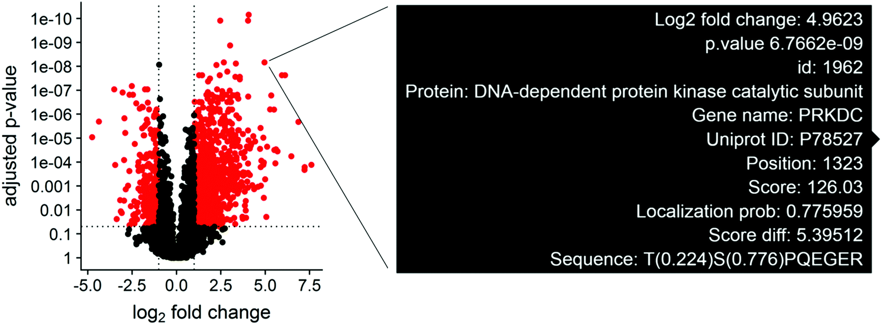

Fig. 2 Interactive view of metadata for significantly altered phosphosites. Phosphosite differential abundance is plotted in a volcano plot for the VAL iCCK1 treatment versus the VAL DMSO control. Hovering over a point renders a text box displaying the protein and gene name, phosphosite position, identification score, localization probability, and flanking amino acid sequence.

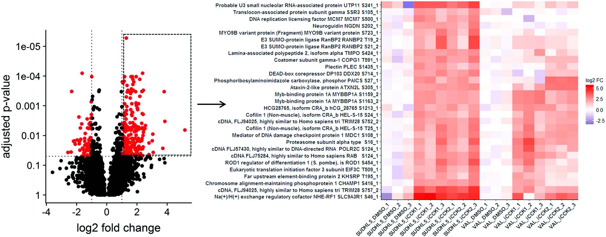Fig. 3 Heatmap of selected phosphosites from Volcano plot. Selecting multiple points from the volcano plot renders a heatmap of these features, allowing for inspection of within-group variance and comparison of differential abundance across additional groups in the data. Upregulated phosphosites, outlined by a box in the volcano plot, from the SUDHL5 iCCK1–SUDHL5 DMSO comparison were selected for plotting a heatmap. The heatmap displays the scaled normalized values. The phosphosite effects were strongly similar in SUDHL5_iCCK2. These phosphosites tend to be upregulated in VAL following iCCK treatment, but are not significant and are inhibitor-specific.

Interactive heatmap

Selecting multiple points from the volcano plot renders a heatmap of quantitative values of the selected phosphosites for all of the samples in the data set (Fig. 3). Heatmaps of the quantitative values for each sample allows for visual inspection of the within-group variance, which is necessary to consider when selecting features for validation studies. Additionally, creating heatmaps of phosphosites from all samples reveals how the differentially abundant features from the specified contrast relate to all samples. For instance, plotting the upregulated phosphosites from the SUDHL5_iCCK1–SUDHL5_DMSO comparison shows that both inhibitors (iCCK1 and iCCK2) exhibit similar effects on the SUDHL5 cell line (Fig. 3). However, the effects on the VAL cell line are more distinct and display an inhibitor-specific effect. The differential cell line response is not surprising since the SUDHL5 cells are derived from a female adolescent lymphoma patient (17 yo) while the VAL cells are from a female adult (50 yo). The differential protein expression patterns from the SUDHL5 – VAL untreated samples were enriched in expected pathways, with the gene ontology terms ovulation cycle process, ovulation cycle, ovarian follicle development, and female sex differentiation among the top six significantly affected pathways. There is an increasing recognition that lymphoma in the adolescent and young adult (AYA) setting has a specific oncogenic signature and an inferior response to therapy compared to adult disease.¹⁶ The unique protein profiles identified in this study supports the capability of proteomic methodologies coupled to ProteoViz for detecting age-related biological differences.

Motif analysis

Protein phosphorylation networks are regulated by kinases and phosphatases, with varying degrees of sequence motif specificity. A frequent question in discovery phosphoproteomics is whether a sequence motif is overrepresented in the list of significantly altered phosphosites. An identified sequence motif may help foster a biological mechanism for the observed results. Several algorithms for sequence motif analysis are described and utilized.¹⁷ The motifx algorithm is the most common algorithm for sequence motif analysis; however, the approach has a tendency to generate false positive results.¹⁸ To enable motif analysis and promote scrutiny of the results, we utilized the rmotifx algorithm to identify overrepresented sequence motifs within phosphoproteomic data sets, and applied a motif filter to relate the statistical output back to the original data. An example data set is shown in Fig. 4. Panel A shows a volcano plot of all quantified phosphosites and the associated sequence logo. Selecting the upregulated region and running motifx yielded a list of significantly overrepresented sequence motifs in this region. The data was then filtered using the motif enrichment parameters box in the dashboard, for two significant sequence motifs Q[ST]P and [ST]P.K, and were plotted in panels B and C. Graphical display of the filtered motifs allows for easier estimation of the magnitude and specificity of the biological effect. The predominant upregulation of the [ST]P phospho-motif is consistent with activation of CDK1/2 kinases, which was also detected in the PTM-signature enrichment for SUDHL5-iCCK1 and SUDHL5-iCCK2. The predominant downregulation of serine phospho-motifs is also consistent with the inhibition of the serine/threonine cell cycle kinase. Additionally, the user interface contains slider inputs to adjust the parameters for the motifx algorithm, including sequence window size and minimum number of sequences for a tested motif. The sequence logos can then be saved and downloaded as a.tiff image of a specified dpi resolution, width, and height.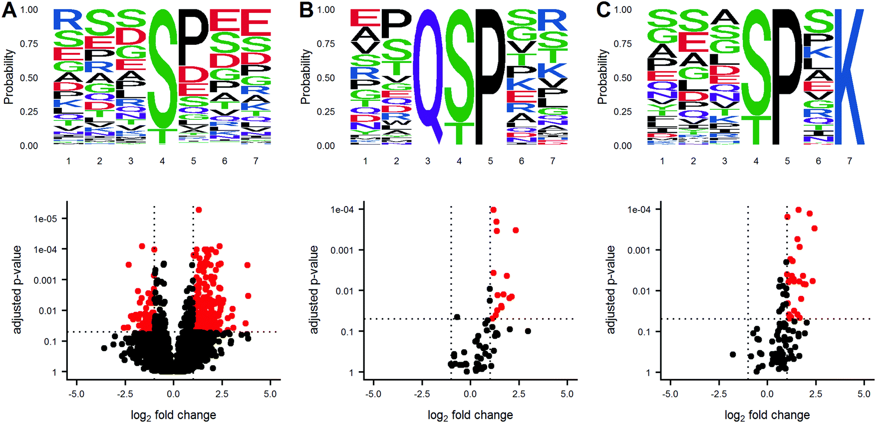

Fig. 4 Graphical output of motifx Sequence motif analysis supplements statistical results. A volcano plot of phosphoproteomics data is displayed in panel A along with the sequence motifs for all peptides. The downregulated region in the volcano plot was selected for sequence motif analysis using the rmotifx library. The data was then filtered for only phosphosites containing the Q[ST]P or [ST]P.K motifs, and the volcano and motifs were replotted in panel (B) and (C), respectively.

Kinase activity and gene set enrichment analysis

A frequent goal of discovery proteomics studies is to identify significantly altered pathways between two experimental conditions. Pathway analysis enables visualization of potential higher-level mechanisms of action underlying the experimental perturbation and may detect minute differences in abundance at the protein level that taken together, manifest in meaningful biological differences. Our platform integrates pathway analysis by utilizing the functions from the EGSEA package to test for significant differences in gene sets from the MSigDB and KEGG resources. The EGSEA results for each experimental contrast are displayed in an interactive heatmap in which pathways are colored based on the aggregated “significance score” from the EGSEA library. By default, only pathways meeting an FDR-adjusted p.value cutoff of 0.05 in at least one contrast are displayed. The heatmap can be adjusted to display specific gene set collections, different significance score cutoffs, and selected contrasts. Clicking on a cell from the EGSEA heat map will generate a heatmap of relative abundances for all proteins quantified in this gene set. For example, the EGSEA results showed that genes from the Fischer G2-M Cell Cycle¹⁹ and the BASSO_CD40_SIGNALING_UP gene sets were significantly altered following iCCK1 or iCCK2 treatment of the SUDHL5 cell line (Fig. 5). The majority of proteins in the G2-M Cell Cycle gene set were upregulated following inhibitor treatment in the SUDHL5 cell line, but are largely unaffected in the VAL cell line. In contrast, the majority of proteins from the Basso CD40 Signaling-Up gene set were upregulated in the VAL cell line following inhibitor treatment. Inspection of the protein differential expression data revealed a significant increase in CD40, TRAF1, and TNFAIP3 following iCCK1 and iCCK2 treatment in the VAL cell line. Thus, clustering and visual inspection of significantly affected gene sets can facilitate mechanistic interpretations of proteomic and phosphoproteomic data sets.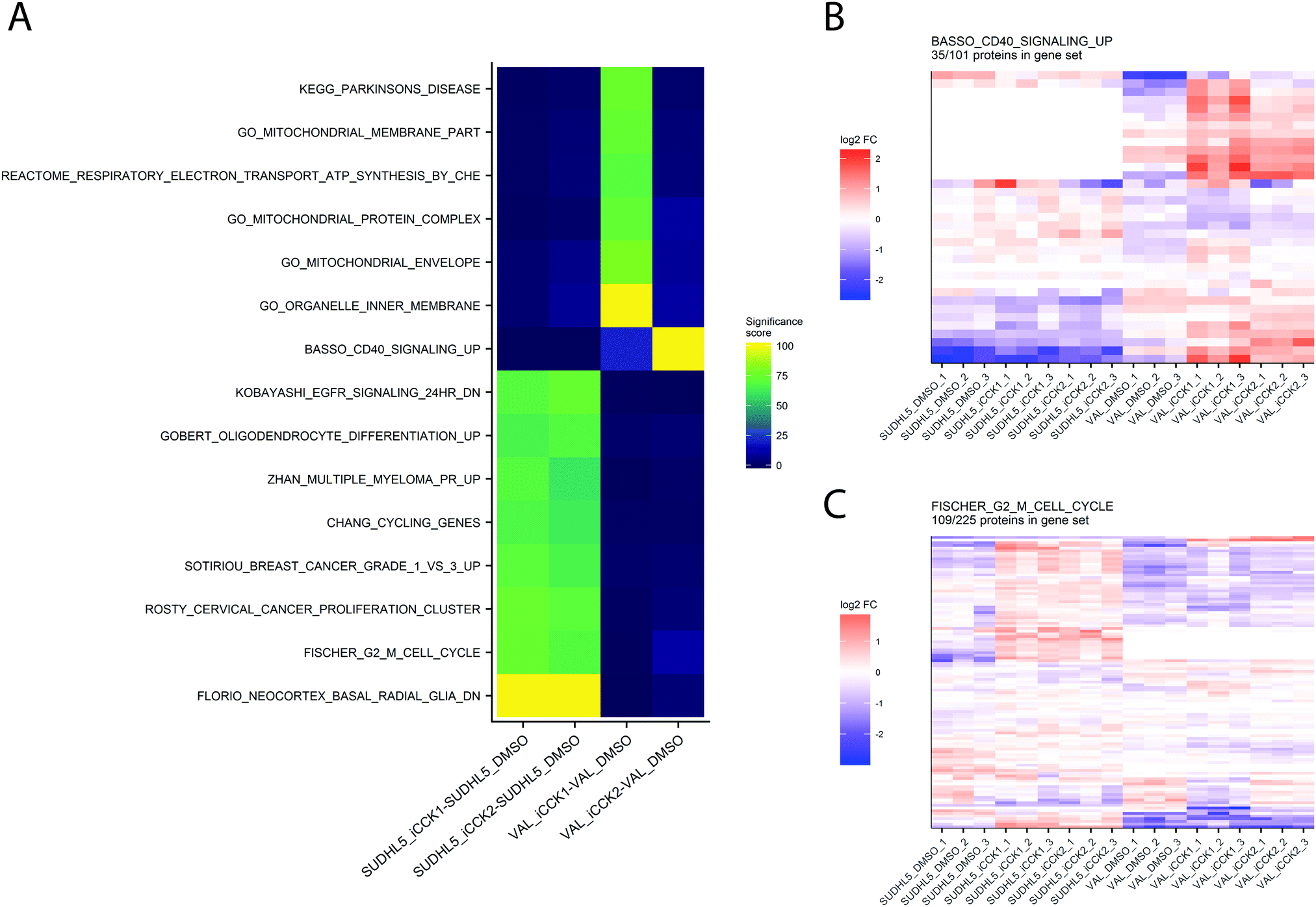

Fig. 5 Inspection of gene set enrichment results. (A) Pathways meeting the significance score for each comparison are displayed in a heatmap. Colors depict the significance score, which aggregates multiple gene set enrichment outputs into a value from 0 to 100. Clicking a region on the EGSEA heatmap renders a relative abundance heatmap for the selected pathway, such as the BASSO_CD40_Signaling_UP pathway (B) and the FISCHER_G2_M_CELL_CYCLE pathway (C).

Conclusions

In this manuscript, we describe and demonstrate the utility of ProteoViz to analyze quantitative phosphoproteomic datasets in an interactive environment to allow for easier biological interpretation. These interactive tools allow researchers to rapidly and efficiently explore complex phosphoproteome data, facilitating discoveries that would otherwise remain elusive.

Although the underlying scripts should be run by bioinformaticians, ProtetoViz was developed with the end user in mind. Its goal is to allocate the data processing to the bioinformatician, and the interpretation and application to the biologist. The most popular current tool for phosphoproteomic analysis is Perseus, which requires thorough expertise in the MaxQuant software and its outputs. Additionally, the Perseus framework requires that the end user performs the data analysis and first learns all of the software requisites. With ProteoViz, the data analysis is handled by a bioinformatician, and the end user only requires a web browser to access the data.

The scripts and example data described in this manuscript provide a framework for analyzing data and building a user interface for investigation of the phosphoproteome. However, the scripts can be modified to incorporate different methods of normalization, new statistical analyses for more complex experimental designs, and customized user interfaces for each project. The workflow can also be modified to use different R packages in order to further customize the plotted outputs. As such, ProteoViz is a powerful tool with the provided scripts serving as a template for a complete, adaptable pipeline for phosphoproteomic analysis.

Data availability

All of the mass spectrometry data is available via ProteomeXchange with identifier PXD015606. The R scripts and example data is freely available at https://github.com/ByrumLab/ProteoViz.

Funding

This study was supported by the Arkansas Children's Research Institute, the Arkansas Biosciences Institute, the UAMS Winthrop P. Rockefeller Cancer Institute Small Grant Seeds of Science Award, the Translational Research Institute (TRI), grant TL1 TR003109 through the National Center for Advancing Translational Sciences of the National Institutes of Health (NIH), and the Center for Translational Pediatric Research funded under the National Institutes of Health grant P20GM121293. The content is solely the responsibility of the authors and does not necessarily represent the official views of the NIH.

Conflicts of interest

No potential conflict of interest was reported by the authors.

Acknowledgements

The authors would like to acknowledge the University of Arkansas for Medical Sciences Proteomics Core Facility and the Arkansas Children's Research Institute Systems Biology Bioinformatics Core Facility.

References

1. F. K. Huang, G. Zhang, K. Lawlor, A. Nazarian, J. Philip, P. Tempst, N. Dephoure and T. A. Neubert, J. Proteome Res., 2017, 16, 1121–1132.
2. A. Hogrebe, L. von Stechow, D. B. Bekker-Jensen, B. T. Weinert, C. D. Kelstrup and J. V. Olsen, Nat. Commun., 2018, 9, 1045.
3. M. HaileMariam, R. V. Eguez, H. Singh, S. Bekele, G. Ameni, R. Pieper and Y. Yu, J. Proteome Res., 2018, 17, 2917–2924.
4. J. R. Wisniewski, A. Zougman, N. Nagaraj and M. Mann, Nat. Methods, 2009, 6, 359–362.
5. D. Wessel and U. I. Flugge, Anal. Biochem., 1984, 138, 141–143.
6. M. W. Senko, P. M. Remes, J. D. Canterbury, R. Mathur, Q. Song, S. M. Eliuk, C. Mullen, L. Earley, M. Hardman, J. D. Blethrow, H. Bui, A. Specht, O. Lange, E. Denisov, A. Makarov, S. Horning and V. Zabrouskov, Anal. Chem., 2013, 85, 11710–11714.
7. G. C. McAlister, D. P. Nusinow, M. P. Jedrychowski, M. Wuhr, E. L. Huttlin, B. K. Erickson, R. Rad, W. Haas and S. P. Gygi, Anal. Chem., 2014, 86, 7150–7158.
8. L. C. Gillet, P. Navarro, S. Tate, H. Rost, N. Selevsek, L. Reiter, R. Bonner and R. Aebersold, Mol. Cell. Proteomics, 2012, 11, O111.016717.
9. B. K. Erickson, J. Mintseris, D. K. Schweppe, J. Navarrete-Perea, A. R. Erickson, D. P. Nusinow, J. A. Paulo and S. P. Gygi, J. Proteome Res., 2019, 18, 1299–1306.
10. F. Ardito, M. Giuliani, D. Perrone, G. Troiano and L. Lo Muzio, Int. J. Mol. Med., 2017, 40, 271–280.
11. K. Krug, P. Mertins, B. Zhang, P. Hornbeck, R. Raju, R. Ahmad, M. Szucs, F. Mundt, D. Forestier, J. Jane-Valbuena, H. Keshishian, M. A. Gillette, P. Tamayo, J. P. Mesirov, J. D. Jaffe, S. A. Carr and D. R. Mani, Mol. Cell. Proteomics, 2019, 18, 576–593.
12. M. Alhamdoosh, C. W. Law, L. Tian, J. M. Sheridan, M. Ng and M. E. Ritchie, F1000Res, 2017, 6, 2010.
13. J. Cox and M. Mann, Nat. Biotechnol., 2008, 26, 1367–1372.
14. G. K. Smyth, Stat. Appl. Genet. Mol. Biol., 2004, 3, 3.
15. D. Schwartz and S. P. Gygi, Nat. Biotechnol., 2005, 23, 1391–1398.
16. J. M. Kahn, N. W. Ozuah, K. Dunleavy, T. O. Henderson, K. Kelly and A. LaCasce, Blood Adv., 2017, 1, 1945–1958.
17. O. Wagih, N. Sugiyama, Y. Ishihama and P. Beltrao, Mol. Cell. Proteomics, 2016, 15, 236–245.
18. A. Cheng, C. E. Grant, W. S. Noble and T. L. Bailey, Bioinformatics, 2019, 35, 2774–2782.
19. M. Fischer, P. Grossmann, M. Padi and J. A. DeCaprio, Nucleic Acids Res., 2016, 44, 6070–6086.

---

Footnote

† Electronic supplementary information (ESI) available. See DOI: 10.1039/c9mo00149b

---