Controlled pharmacokinetic anti-cancer drug concentration profiles lead to growth inhibition of colorectal cancer cells in a microfluidic device

Abstract

We present a microfluidic device to expose cancer cells to a dynamic, in vivo-like concentration profile of a drug, and quantify efficacy on-chip. About 30% of cancer patients receive drug therapy. In conventional cell culture experiments drug efficacy is tested under static concentrations, e.g. 1 μM for 48 hours, whereas in vivo, drug concentration follows a pharmacokinetic profile with an initial peak and a decline over time. With the rise of microfluidic cell culture models, including organs-on-chips, there are opportunities to more realistically mimic in vivo-like concentrations. Our microfluidic device contains a cell culture chamber and a drug-dosing channel separated by a transparent membrane, to allow for shear stress-free drug exposure and label-free growth quantification. Dynamic drug concentration profiles in the cell culture chamber were controlled by continuously flowing controlled concentrations of drug in the dosing channel. The control over drug concentrations in the cell culture chambers was validated with fluorescence experiments and numerical simulations. Exposure of HCT116 colorectal cancer cells to static concentrations of the clinically used drug oxaliplatin resulted in a sensible dose-effect curve. Dynamic, in vivo-like drug exposure also led to statistically significant lower growth compared to untreated control. Continuous exposure to the average concentration of the in vivo-like exposure seems more effective than exposure to the peak concentration (C_max) only. We expect that our microfluidic system will improve efficacy prediction of in vitro models, including organs-on-chips, and may lead to future clinical optimization of drug administration schedules.

---

Introduction

Cancer is the number two cause of death worldwide. About 30% of cancer patients receive drug therapy, dependent on cancer stage.¹ Drug concentration in blood and tissues is dynamic; it first increases after administration and declines due to distribution, drug metabolism and excretion.² These varying concentrations, or ‘pharmacokinetics’ are an important aspect of the efficacy of a treatment and the ideal dosing regimes to control concentrations of a therapeutic in patients are an intense topic of clinical research.³ In contrast, in vitro, novel drugs are tested on cultured cells in a time-constant concentration, e.g. 1 μM for 48 hours,⁴ and this lack of realistic dosing regimes contributes to the poor correlation of in vitro results with observations in the clinic.⁵

Certain pharmacokinetic parameters of clinically relevant drug exposures are available and can in principle be used to inform the static drug concentrations used in cell culture studies.⁶ For example, maximum concentration in blood (C_max) values can be used to set the maximum concentration of a drug for in vitro experiments. Alternatively, drug half-life (t_1/2) and total drug exposure over time (area under the curve, AUC) can be used to inform approximate drug exposure durations.

Nevertheless, it cannot be known beforehand whether either the C_max, t_1/2, AUC, and/or a combination, is the pharmacokinetic driver of drug efficacy, as this depends on drug characteristics such as diffusion, binding and mechanistic effects. For many drugs the pharmacokinetic–pharmacodynamic (drug efficacy) correlation often remains a topic of discussion, as illustrated by the debate on the widely used anti-cancer drug cisplatin.⁷ As pharmacokinetic parameters of drugs are correlated, e.g. by increasing the dose, both C_max and AUC increase, isolating the pharmacokinetic driver of efficacy can be a challenge. A partial solution is dose fractioning in animals,⁸ however this is resource-intensive and there are limits to dosing frequency for animals. Due to these challenges and lack of in vitro testing possibilities, a final resort is trial and error in humans. For example, the anti-cancer drug oxaliplatin, a first line therapeutic for metastasized colorectal carcinoma in a schedule with 5-fluoruracil and leucovorin, is sometimes administered with a prolonged infusion time of 6 hours instead of 2 hours, thereby lowering C_max, to reduce side effects.^9,10

Hence, it would add a lot of value to in vitro studies if it were possible to not simply pick a single static concentration and exposure time, based on some of the pharmacokinetic parameters, but instead to have full control over the dynamics of drug concentrations. This could also accelerate the adoption of the FDA of advanced in vitro models into the drug development regulatory pathway.¹¹

Conventional technical solutions to mimic in vivo concentrations in vitro have been developed, for example dynamic flow chamber set-ups or hollow fibre models for antibiotics. However, drawbacks of these systems are high reagent use, low throughput and membrane blockage.¹²

Microfluidic technology is ideally suited to overcome these challenges.¹³ Mimicking in vivo-like drug concentrations over time, on-chip, is an emerging field where pioneering work has been done on antibiotics and kidney toxicity.^14,15 While cancer drug testing has been performed extensively in microfluidic cell culture systems,^16–19 mimicking in vivo-like drug concentrations over time on-chip has up to recently been largely neglected in the oncology field, with recent notable exceptions.^20–23 Several current solutions rely on active perfusion of cell culture chambers with dynamic drug concentrations.^22,23 This perfusion results in shear stress, which increases with a higher concentration change rate. Systems in which cells are cultured in a separate compartment to prevent direct exposure to fluid flows suffer from other drawbacks. For example, cells are cultured directly on a membrane, which hampers visual inspection, or specific geometries limit concentration rate change or concentration range.^14,15,20,21

Lohasz et al. defined a hypothetical in vivo-like concentration profile for the non-clinical drug staurosporine and controlled its concentration on-chip through gravity-driven flow controlled by chip tilting and a specific chip geometry.²⁰ Chou et al. administered a flat (investigative) drug dosage which stopped after two hours, and the diffused drug in the tissue channel acted as a reservoir to provide the drug for the declining concentration phase.²¹ Although these technical solutions are sophisticated, its strong reliance on microfluidic chip geometry might limit broad adoption and puts constraints on dosing schedules. Guerrero et al. used two microfluidic pumps to administer a dynamic drug dose in a one layer chip. Two clinically approved drugs, doxorubicin and gemcitabine, were administered to breast cancer cell line cells at in vivo-like concentrations.²²

To prevent shear stress, as this is often absent in interstitial tumor tissue due to deficient lymphatic drainage and increased interstitial and oncotic pressure,²⁴ we developed and characterized a two layer chip with a membrane for dynamic drug concentrations. Dynamic drug concentrations are administered by pre-programmed syringe pumps. This solution allows for freedom in the design of the microfluidic chip and is widely applicable to organ-chip systems. Moreover, cells are seeded not at the membrane but at the bottom, which allows for on-chip, label-free, pre-post quantification of cell growth of a single culture condition.

Here, we use our microfluidic system to investigate the in vitro effect of oxaliplatin on colorectal cancer cells.² Oxaliplatin was chosen as a model drug as it is a first line drug in the treatment of colorectal cancer, one of the most frequent cancers.¹⁰ We also use the results of our assay to explore the pharmacokinetic driver of efficacy of oxaliplatin at an in vivo-like dosage.

Experimental

Device design and fabrication

The microfluidic device consists of two crossing channels, a (bottom) culture channel containing the cells and a so called (top) treatment channel for drug dosing, separated by a membrane (Fig. 1a). The cross shape allows for seeding cells at the intersection of the channels, below the membrane in a controlled manner (Movie S1†). After seeding the cells in the bottom channel the bottom channel is closed to enable shear stress free dynamic drug exposure. Dynamic drug dosing is provided via changing the drug concentration in the top channel via two separate syringe pumps and subsequent diffusion of drug to the bottom channel via the membrane. The membrane is a 35 μm thick transparent hydrophilic polytetrafluorethylene (PTFE) membrane purchased from Sterlitech (US), consisting of random fibres which block particles >1 μm, and with a typical empty volume of ∼80%. The bottom layer is glass for cell adherence and growth, other layers are made out of polydimethylsiloxane (PDMS) for oxygen diffusion in static experiments. Channel dimensions are 17 × 2 × 0.5 mm and 21 × 2 × 1 mm for the bottom (culture) and top (treatment) channel respectively, to allow for sufficient nutrients in static conditions and sufficient cell numbers for quantitative analyses.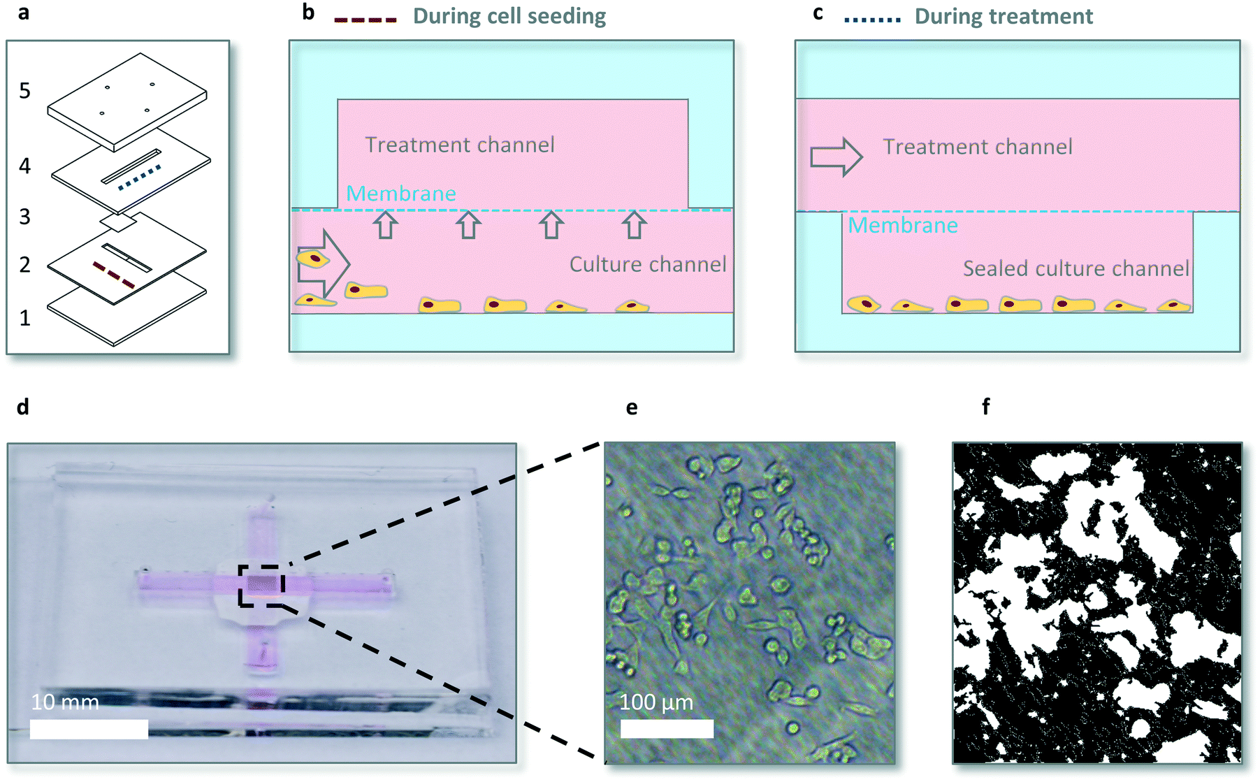

Fig. 1 Microfluidic chip design and function. (a) Multilayer cross channel chip design; glass (1), PDMS (2), PTFE membrane (3), PDMS (4 and 5). Dashed blue and brown lines represent cross section view direction for b and c respectively. (b) Cells in the bottom channel are seeded exclusively below the membrane, at the intersection of the top and bottom channel by forcing flow over the membrane by blocking the outlet of the bottom channel when introducing cells. (c) Drug is administered in the treatment channel, separated by a PTFE membrane from the closed bottom channel, to prevent shear stress while maintaining diffusion and optical transparency. (d) Photograph of the device filled with medium. (e) Brightfield microscope image of adhered cells on the bottom of the device below the membrane and (f) confluency algorithm (see ‘Growth inhibition experiments’ paragraph) translation for quantification.

Chips were fabricated using PDMS in a 1 : 10 weight ratio of base vs. curing agent (Sylgard 184, Dow Corning, US). The PDMS was poured on a mould, degassed, and cured at 60 °C overnight. For the top channel, a micro milled (Datron Neo, Germany) mould was used. For the bottom channel, a flat silicon wafer-based mould with subsequent press-cutting (Bleijenberg, The Netherlands) of the channel geometry was used. The chips were bonded to glass microscope slides after activation by oxygen plasma using a plasma cleaner (model CUTE, Femto Science, Germany). PDMS parts and membrane were glued by using a mixture of toluene and PDMS at a 2 : 3 ratio and were allowed to bond overnight. Inlet and outlet holes were punched using Harris UniCore punchers of 1 mm diameter.

For static condition treatments, Tygon (Cole Palmer, US) tubing with a 0.05′′ inner diameter was connected to the inlets and outlets of the chip, and for dynamic experiments, 1/16′′ outer diameter, and 1/32′′ inner diameter Teflon tubing, with an IDEX (US) P712 Peek flow splitter was used.

Microfluidic dynamic drug exposure characterization experiments

The ability to control dynamic drug concentrations in the chip was verified by fluorescein experiments and oxaliplatin measurements. To evaluate lag induced by dead volume, two programmable syringe pumps were used (Harvard PhD2000, US), one of which holding a 10 ml syringe (B. Braun, Germany) with 10 μM fluorescein sodium salt (molecular weight, 332 Da, Sigma-Aldrich, US) in phosphate-buffered saline (PBS) and one with only phosphate buffered saline (PBS). Tubing was combined with a flow splitter, with the combined tube connected to the chip. The administration schedule covered the (relative) dosing steps and absolute flow rates of the administration schedule used for cell experiments, with dosage steps of fluorescein of 5, 2, 1.0, 0.3 and 0 μM with flow rates of 10, 10, 3, 3, 3 μl min⁻¹, for 15, 15, 30, 30, 60 minutes respectively. Fluorescence images were obtained with a green filter (GFP) fluorescence microscope (Leica DM IRM, Germany). Quantification of fluorescence was done in ImageJ software.²⁵ For quantification of fluorescence a fixed location and fixed exposure time per time series is used, and background fluorescence was subtracted.

The time to achieve a stable concentration of fluorescein in the top channel for different flow rates was evaluated with 5 μM fluorescein in the top channel on the inlet side, before the membrane, at flow rates of 3, 10, 30 μl min⁻¹. Flow rates were chosen to cover the relevant flow rates and explore a potential relation between flow rate and time to achieve a stable concentration. Time measurements were corrected for dead volume after the flow splitter (see Fig. 2).

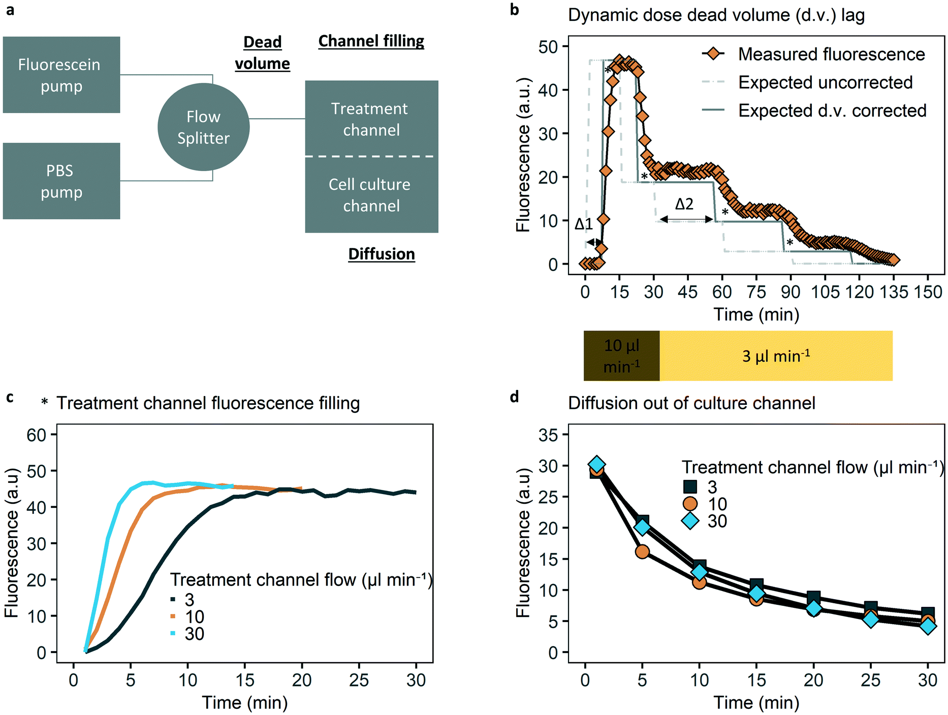Fig. 2 Dynamic drug control characterization. (a) Schematic overview of the dynamic solute control chip-system and factors influencing control; dead volume, channel filling, diffusion time. (b) Dynamic drug concentration control in the top (treatment) channel is affected by dead volume (∼85 μl). There is a (varying) time lag due to dead volume, as shown between uncorrected expected and corrected (for dead volume) expected fluorescence. An initial dead volume time of ∼8 minutes (Δ1) arises when starting with PBS between the flow splitter and chip, and additional dead volume time of ∼20 minutes (Δ2) after flow rate decrease from 10 to 3 μl min⁻¹. Measured fluorescence follows expected corrected fluorescence closely, except for lags marked with an asterisk, which are the result of Taylor dispersion. (c) Due to Taylor dispersion there is a time lag until the top channel solute concentration equilibrates. Top channel equilibrium time decreases in flow speed, with about six minutes for 10 μl min⁻¹. (d) Diffusion quantification of fluorescein over the membrane and bottom channel. 50% fluorescence decrease within 5–10 minutes at the membrane area independent of (relevant) flow speeds after loading the bottom channel with fluorescein and flowing PBS through the top channel.

Diffusion across the membrane was evaluated by loading the bottom channel with 5 μM fluorescein in PBS with a closed top channel with PBS, closing the bottom channel via plugs in the bottom channel inlet and outlet, and then continuously flowing PBS across the top channel at 3, 10, 30 μl min⁻¹ while quantifying decline of fluorescence over time in the bottom channel.

To validate fluorescein as a model for oxaliplatin diffusion, the top channel was loaded with both, and after 16 hours, diffusion into the bottom channel was measured with UV-vis spectrophotometry (Thermo Fisher Nanodrop 2000, US). Starting concentrations were 200 μM and 6.25 mM respectively, so measured values would be in the range of the spectrophotometer based on calibration curves of fluorescein and oxaliplatin (Fig. S1†).

PDMS is known to potentially adsorb and absorb molecules, especially small lipophilic molecules.²⁶ To verify no significant sorption, oxaliplatin at 30 μM was flushed through the top channel for 30 minutes at 10 μl min⁻¹, collected, and analysed with UV-vis spectrophotometry.

For determining oxaliplatin in the top channel outlet, the concentration of platinum (Pt) was measured with a 8300DV ICP-OES (Perkin Elmer, US). The calibration standards for Pt was made by diluting a standard solution (Merck, Certipur, 1000 mg L⁻¹ Pt) with PBS.

Numerical simulations of drug concentration over time

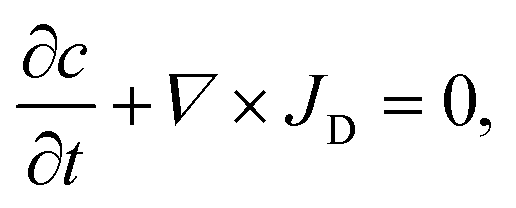
Two-dimensional diffusion equation simulations were performed with Comsol 5.1 (Comsol AB, Burlington, MA). The equation solved is the continuity equation;
with for the flux, J_D, diffusion according to Fick's law;

J_D = D∇c,

with D, the diffusion coefficient and c the concentration of the solute, with a no-flux boundary condition at the channel walls. The flux through the membrane was modelled as the boundary condition:
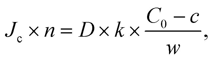
with, C₀ the concentration in the top channel, k, the permeability constant of the membrane and w the thickness of the membrane. The flow velocity in the top channel was considered to be sufficiently high to neglect the local depletion in the top channel just above the membrane.

Chip geometries were used, in 2D, assuming a closed system (Fig. S8†). For fluorescein, with a molecular weight of 332 Da, a known diffusion from the literature of 4.2 × 10⁻⁶ cm² s⁻¹ was used, on the lower side of the range of estimates of 4.0–5.7.²⁷ For oxaliplatin, with a comparable molecular weight of 397 Da, the diffusion coefficient is unknown. Based on a similar diffusion in the chip as fluorescein (Fig. S1†) we used the same diffusion coefficient for oxaliplatin for simulations. This is likely a conservative diffusion coefficient as cisplatin, with a more similar molecule structure to oxaliplatin, at molecular weight of 300 Da, has an estimated diffusion coefficient of 8.2 × 10⁻⁶ cm² s⁻¹.²⁸

The optimal value of k (0.2) was determined by fitting the model to experimental data from the diffusion experiment (Fig. 2d and S10†). Flow in the top channel was assumed infinite for finding the membrane characteristics and dynamic drug dosing, based on relatively large flow of 3, 10, 30 μl min⁻¹ in experiments.

With the permeability constant found from the diffusion experiment, the drug exposure to cells on the bottom of the bottom channel with a given dosage schedule was simulated using the same computational model.

Growth inhibition experiments

HCT-116 colorectal cancer cells (Sigma-Aldrich) were cultured in McCoy 5A medium (ThermoFisher) with 5% foetal bovine serum (FBS, ThermoFisher) and 1% penicillin–streptomycin (ThermoFisher) and used at passage numbers under 30. For experiments, 3000 cells were seeded for a 25% (Fig. S16†) starting surface coverage of the bottom channel and concentrated under the membrane, via forced fluid flow of 20 μl min⁻¹ through the membrane. After cell localization under the membrane, the bottom channel was closed with plugs.

Cells attached overnight and were subsequently treated for 48 hours with static or dynamic concentrations of oxaliplatin (Sigma-Aldrich, US), or medium as a control. All experiments were performed in a cell culture incubator.

Medium, drug, and staining were administered in the top channel with a syringe pump, or two programmable pumps for dynamic drug concentrations as described above. Static treatment consisted of a flush of 10 μl min⁻¹ for 20 minutes through the top channel and 48 hours incubation. The dynamic dosing schedule of oxaliplatin was based on mice pharmacokinetics, as mice pharmacokinetics are often available at an earlier stage in the drug discovery process than human pharmacokinetic data. Pharmacokinetics found in a study using 8 mg kg⁻¹ oxaliplatin dosage were used.² This dosage is a midpoint in the standard dosage range of 5–10 mg kg⁻¹.^29–31 The in vivo pharmacokinetics are used as a starting point. With one pump containing 60 μM oxaliplatin in medium, and one pump with medium, combinations of flow rates are programmed to match the in vivo pharmacokinetics, taking chip mass transport characteristics into account.

Cell growth was quantified before and after treatment by a label-free confluency analysis³² and expressed relative to starting confluence. Brightfield images were obtained at 10× magnification (Leica DM IRM, Leica Microsystems, Wetzlar, GmbH, Germany). Images were split into individual red-green-blue (rgb) channels, and the green channel images were stitched in ImageJ/FIJI.³³ The stitched images were evaluated with the PHANTAST segmentation algorithm at standard settings of sigma 1.20 and epsilon 0.03. Corrections for background signal were made by sampling three areas without cells and subtracting this from the confluency number. Growth was expressed relative to average control growth in the following manner:

where n is the number of control experiments. Results were pooled per control and treatment condition to have 3 or more chips in total per condition from at least two independent, i.e. executed on a different date, experiments. Statistical significance is tested with an analysis of variance (ANOVA) test and subsequent Tukey HSD test for individual conditions, in software package R version 3.6.3.

CalceinAM (ThermoFisher) at 10 μM was used for assessing overall viability, ethidium homodimer (ThermoFisher) at 10 μM for late apoptotic cells and NucBlue (ThermoFisher) at 8 drops per ml for nucleus identification. Fluorescence images were obtained with GFP, Texas Red, DAPI filter (ThermoFisher EVOS) at 10×.

For 96-well validation experiments, 10 × 10³ cells in 100 μl medium were seeded per well, attached overnight and treatment added for 48 hours in 100 μl medium. Growth was quantified with confluency analyses as described above.

Results and discussion

Microfluidic device design and cell seeding

The microdevice that we designed for our studies contained two intersecting channels, separated by a transparent porous membrane (Fig. 1). The top channels serves as the treatment channel via active fluid flow, whereas the bottom channel remains static and serves as the cell culture channel. Dynamic drug concentrations are created by two separate programmable syringe pumps. Tubing from these two pumps is combined via an Y splitter and connects to the top channel. Cells were seeded and analysed exclusively at the intersection of the channels. To hold enough cells to limit spiking errors and stochastic drug responses, a bottom and top channel width of 2 mm, and therefore a culture area of 4 mm², was chosen. This allows for culturing thousands of cells at full confluency. In order to expose cells to dynamic drug concentrations, diffusion time should be relatively short from the top channel to the bottom cell culture area. We therefore designed a microfluidic system which has a bottom channel of limited depth (0.5 mm). The top channel has a depth of 1 mm, which combined with the bottom channel of 0.5 mm, satisfies the 1.2 mm medium column per 48 hours rule of thumb for sufficient nutrients in static experiments.³⁴ For seeding, 3000 cells in 5 μl were manually pipetted in the bottom channel and were allowed to sink for 1–3 minutes. Then a flow rate of 20 μl min⁻¹ was applied as cells then have sufficient horizontal speed to locate under the membrane, but upward flow is insufficient for lifting the cells from the bottom (Movie S1†).

Controlling dynamics of solute concentrations inside the microfluidic chip

To study the control over the dynamic concentration of the small molecule drug oxaliplatin in the top channel of the chip we measured oxaliplatin in the outlet. The oxaliplatin concentration measured in the outlet follows the administered oxaliplatin well, with a deviation of less than 10% (Fig. 3a). As the bottom channel is a sealed compartment, a direct measurement would require local concentration sensing in the culture area, which is not practically feasible for oxaliplatin and other drugs. Therefore, we took the approach of tracking fluorescein, a fluorescent molecule which behaves similar to the solute of interest, as an alternative for direct sensing. To verify comparable diffusion characteristics for fluorescein and oxaliplatin, a static diffusion experiment was conducted, in which the top channel was loaded with oxaliplatin and fluorescein, while the bottom channel was loaded with PBS, and after 16 hours the bottom channel was flushed and analysed with UV-vis spectrophotometry. Relative diffusion of both solutes was equal from the top to the bottom channel (Fig. S1†).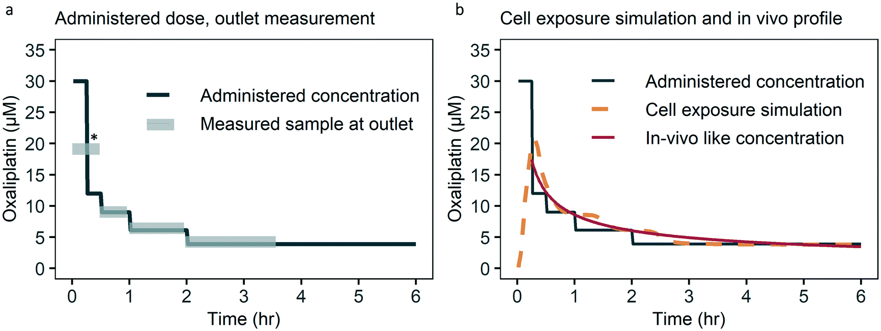

Fig. 3 Administered, measured, simulated oxaliplatin concentration over time. (a) The measured concentration in the outlet is within 10% of the administered concentration. Deviation from the administered concentration at * is due to collection of medium at the outlet for the first 30 minutes which combines the 30 and 12 μM steps, due to the detection limit. For the timing of sample collection taking dead volume into account see Fig. S3.† (b) Cell exposure is based on a numerical simulation taking into account drug administration, dead volume, channel filling and diffusion lag. Cell exposure follows the in vivo like drug concentration over time closely. First six hours of 48 hour infusion schedule shown for optical clarity.

PDMS allows for static drug exposure which is methodologically closest to 96 well experiments, thereby providing an intermediate step between well plate experiments and dynamic/continuous flow chip experiments. However PDMS is known to absorb certain drugs,²⁶ nevertheless oxaliplatin is not suspect for PDMS sorption based on lipophilicity as expressed by octanol/water coefficient (log P) of −0.47.^35–37 With UV-vis spectroscopy we detected no absorption of oxaliplatin (Fig. S2†).

By applying fluorescein as a model compound, we studied the time resolution of dynamic solute control, focusing on three key parameters: dead volume lag time, equilibrium time of the top channel and diffusion time to the bottom channel (Fig. 2).

Dead volume lag time is defined as the time needed for a new concentration of the solute to travel from the flow splitter to the top channel over the cell culture area. Dead volume comprises the volume of the common inlet tubing (75 μl) and the first part of the treatment channel (10 μl). At a flow rate of 10 μl min⁻¹ there would be a delay of about 8 minutes for the fluorescence signal to start, while at a flow rate of 3 μl min⁻¹ this lag time would be about 28 minutes. This was also confirmed by measurements of the dead volume lag times in the system (Fig. 2b). The potential delay caused by hydraulic resistance and capacitance is assumed insignificant compared to the dead volume time and required dosing time steps.

It also takes time to homogeneously fill the top channel with the solute (Fig. 2c). This equilibrium time is a result of a parabolic flow profile in a square channel cross-section causing Taylor dispersion of the solute along the channel axis. These lags are flow rate dependent, as equilibrium is achieved in 4, 6, 15 minutes for 30, 10, 3 μl min⁻¹ respectively (Fig. 2c).

After reaching equilibrium, variation in fluorescence over the width of the channel is within 10%, illustrating the homogeneity in the distribution of solute upon entry into the chip (Fig. S4, S5 and S7).

To characterize the diffusion time to the bottom channel, the bottom channel of the chip was loaded with fluorescein. Any fluorescein diffusing into the top channel was washed out by perfusing the top channel with PBS. A decrease of 50% of fluorescence was observed within 10 minutes, independent of which perfusion rate was chosen for the top channel (Fig. 2d). Remaining fluorescence after thirty minutes is due to diffusion out of the areas of the bottom channel adjacent to the cell culture area. Fluorescent images supporting the data in Fig. 2, as well as a comparable analysis for the fluorescent drug doxorubicin are provided in Fig. S4–S6 and S13–S15.†

As dead volume lag can be controlled for, and the combination of a typical top channel equilibrium time of 6 minutes with a diffusion time to the bottom channel of less than 10 minutes for a 50% concentration reduction, the typical half-life for fluorescein (and thus oxaliplatin) that we can achieve in our system is within 20 minutes.

Delivering a pharmacokinetic concentration profile to the microfluidic cell culture chamber

To expose cultured cells in a microfluidic chip to oxaliplatin concentration profiles that match the in vivo pharmacokinetics, a short peak of 20 μM needs to be given which declines over several hours to a lengthy exposure of 1–2 μM (Fig. S17†).² Distribution half-life of oxaliplatin, i.e. the time it takes from the peak dose to halve, based on distribution of the drug from the vascular space to the tissues, is ∼20 minutes. This is the most constraining drug concentration change, as a rapid rise can be induced by using a higher concentration, while decline is limited by zero concentration in the top dosing channel. Therefore distribution half-life can be used as the minimally required rate of concentration change for the chip-system. In the previous section it was shown our chip can indeed achieve 50% of concentration reduction within 20 minutes.

The pump programming schedule for delivering oxaliplatin to the cell culture chamber is based on the drug concentrations found in vivo, taking dead volume, channel equilibrium lag times and diffusion into account. During phases of peak exposure and distribution half-life, a flow of 10 μl min⁻¹ was used to reduce top channel equilibrium time, whereas for the remaining time a lower flow rate of 3 μl min⁻¹ was used to conserve medium. The decrease in flow rate was programmed after 1 hour to prevent extension of dead volume time to coincide with a required steep concentration decline. The lower flow rate still supplies an abundance of oxygen and nutrients.^34,38

As C_max peak exposure of 20 μM occurs after 15 minutes, there is a need to administer a higher starting concentration dose of 30 μM as the diffusion assay (Fig. 2) indicated that after 15 minutes 2/3rd of the fluorescein has diffused out, which should mirror loading solute into the culture area.

Importantly, control over drug concentrations in the cell culture chamber still needs to be translated to local concentrations in the bottom of the chamber, where the adhered cancer cells will grow. To estimate cell exposure in the microfluidic chip with the programmed pumping, a numerical simulation was used. As the membrane has a random fibre like structure, experimental diffusion results from the diffusion assay (Fig. 2b) were used to find an equivalent large pore membrane with equal thickness with numerical simulations. The best fit with experimental data from the diffusion assay was obtained by using 20% (k = 0.2) porosity (Fig. S10†).

The modelled membrane was used as an input in a numerical simulation of drug exposure of cells on the bottom of the bottom channel, along with the following assumptions: diffusion coefficient of oxaliplatin of 4.2 × 10⁻⁶ cm² s⁻¹, which is equal to fluorescein based on diffusion experiments (Fig. S1†), and top channel concentrations follow the administration schedule with drug concentrations adjusted for concentration change lags based on used flows.²⁷

The numerically simulated cell exposure follows the in vivo blood concentrations measured (Fig. 3b). Deviation on key pharmacokinetic parameters such as the area under the curve (AUC), AUC of the first hour and the C_max are within 20%, which we deem acceptable given the biologic variation observed within and between studies and species.^2,39 The current approach of an administration schedule based on the in vivo-like concentration, taking into account lags in concentration change, works well. In the future we do envision a formal transfer function to further ease translation of the desired dynamic drug concentration to an administration schedule.

A limitation of the system is the inability to measure drugs directly under the membrane in the cell culture area. To ensure sufficient diffusion of the molecule to the cell culture area when using a different drug than oxaliplatin, non-absorbance and transport through the membrane and bottom channel should be tested (Fig. 3a and S1, S2 and S11†). The system is primarily intended for small molecule drugs, typically with a molecular weight up to 1500 Da, and diffusion coefficients in the range of 2.9–9.0 10⁻⁶ cm² s⁻¹.⁴⁰ Diffusion coefficients within this range have a limited influence on diffusion time towards the cell culture area of less than 5 minutes, which is acceptable depending on the in vivo pharmacokinetic profile (Fig. S12†).

Static oxaliplatin cancer cell growth inhibition in the microfluidic chip

The developed microfluidic chip allows us to expose cancer cells to controlled concentration profiles of oxaliplatin, including those that mimic pharmacokinetics of the drug in vivo. The colorectal cancer cell line HCT116 was seeded in the cell culture area of the bottom channel, and its growth was tracked by brightfield microscopy. Methodologically closest to standard laboratory 96 well growth inhibition is static exposure. Static exposure on chip leads to a sensible dose response effect, i.e. reduction of HCT116 cell growth in increasing dosages of oxaliplatin (Fig. 4a). For 48 hours of 0 (control), 1, 10, 100 μM oxaliplatin exposure, growth versus control is 100%, 100%, 40%, 10% respectively. The effect of the drug is statistically significant for 10 and 100 μM oxaliplatin versus control. Starting confluency for control, 1, 10, 100 μM oxaliplatin were between 0.2 and 0.3 on average for all conditions and differences were not statistically significant (Fig. S16†).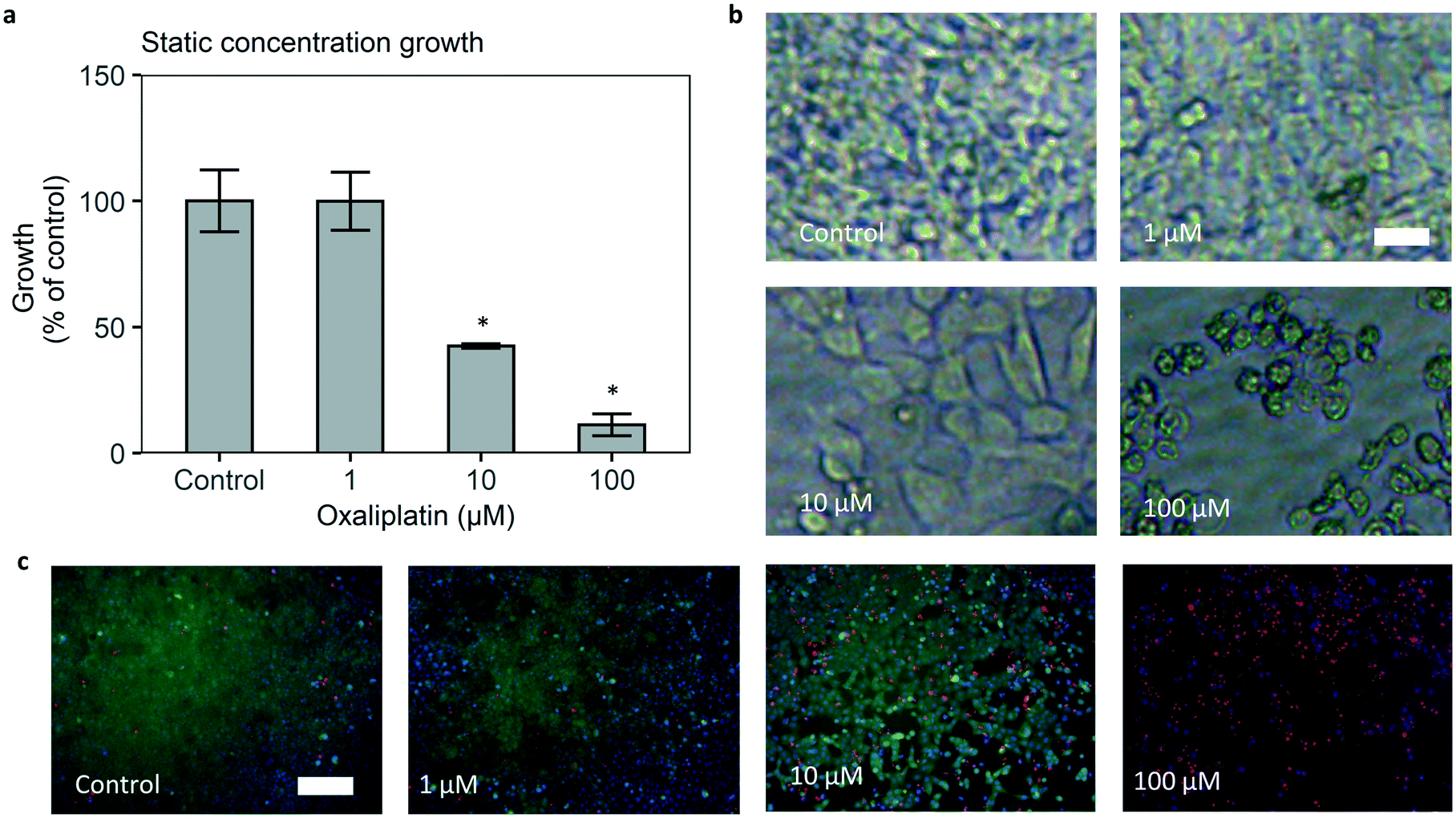

Fig. 4 Treatment of human colorectal cancer cells in the microfluidic chip with static concentrations of oxaliplatin leads to growth inhibition and cell death. (a) Average 48 hour confluency growth relative to control is 1.0 for control, 1.0 for 1 μM, 0.4 for 10 μM, 0.1 for 100 μM. Error bars are standard error of the mean (SEM). N = 3–5 per treatment condition. *p < 0.05 versus control. (b) Brightfield images show lower cell density and less spreading with increasing dosages. Scale bar 20 μm. (c) Staining shows lower growth and increasing apoptosis with higher concentrations, and general loss of viability at 100 μM; cell nuclei (NucBlue/Hoechst 33342, blue), viability (calcein AM, green), late stage apoptosis (ethidium homodimer, red). Scale bar 200 μm.

To confirm the dose–response effect, a calcein/ethidium homodimer (‘live–dead’) staining after drug exposure was performed. The results showed lower growth and higher late stage apoptosis at 10 and 100 μM oxaliplatin and a general loss of viability at 100 μM oxaliplatin (Fig. 4c).

It must be noted that static on-chip administration of oxaliplatin leads to an effective dose that is 25% lower than the administered dosage. This is due to the fact that the drug is only introduced in the top channel, after which it diffuses into the bottom channel, thereby diluting the administered dose.

On-chip cell growth versus control was comparable to internal and external 96 well results for 10, 100 μM oxaliplatin (Fig. S18†).⁴ Growth versus control for 1 μM oxaliplatin treatment is higher on chip. Besides the 25% lower actual drug concentration in the cell chamber, this is primarily driven by a lower growth rate of cells under control conditions in the chip (Fig. S18†).

Altered baseline cell growth in microfluidic devices versus macroscale culture is common.⁴¹ A specific potential explanation for our chip system is that a confluency read-out based on brightfield microscopy typically underestimates cell numbers at high confluency.⁴² This effect is more pronounced with less homogeneous seeding, which could occur on chip compared to 96 well plates. This explanation is supported by the observation that a typical control confluency increase of 20% to 50% (2.5×) based on analysis of brightfield images is matched by a 3.5 fold increase in cell nuclei (Fig. S19†).

Other potential, but more difficult to quantify, factors could contribute to the control growth difference. Besides less confluency growth compared to DAPI nucleus count based growth, less homogeneous seeding can also lead to slower actual cell growth. Also PDMS can leach uncured molecules and absorb growth factors, which has been implicated in lower microfluidic baseline cell growth.⁴¹

A comparison to macroscale culture helps understand the effect of the microfluidic chip system on cell growth (inhibition) versus a 96 well plate. However 96 well plate results are an imperfect gold standard for both control and treated tumour growth as in vivo, tumours grow much slower than in well plate experiments. As an indication, an estimate of tumour doubling times for colorectal carcinoma is 4 months, while doubling time in a 96 well plate for HCT116 colorectal cancer cells is 21 hours.^4,43

In summary, the chip-system displays a clear dose response effect for oxaliplatin which corresponds well with 96 well results, albeit with a lower sensitivity for (sub) micromolar oxaliplatin concentration. Still, the growth reduction sensitivity at dosages higher than 1 μM provides the opportunity to test in vivo-like drug concentrations.

Growth inhibition by in vivo-like concentrations of oxaliplatin in the microfluidic chip

To test the effect of an in vivo-like concentration of oxaliplatin, published pharmacokinetic data of oxaliplatin blood concentration over time were translated into a drug administration schedule and infused into the chip treatment channel by syringe pumps (Fig. 5a and S17†).² Cell growth relative to control is 60% of control (Fig. 5c). The difference is statistically significant with a significance of p < 0.05. Hence the microfluidic chip-system is able to detect a significant growth reduction when applying an in vivo-like concentration of a clinically approved drug.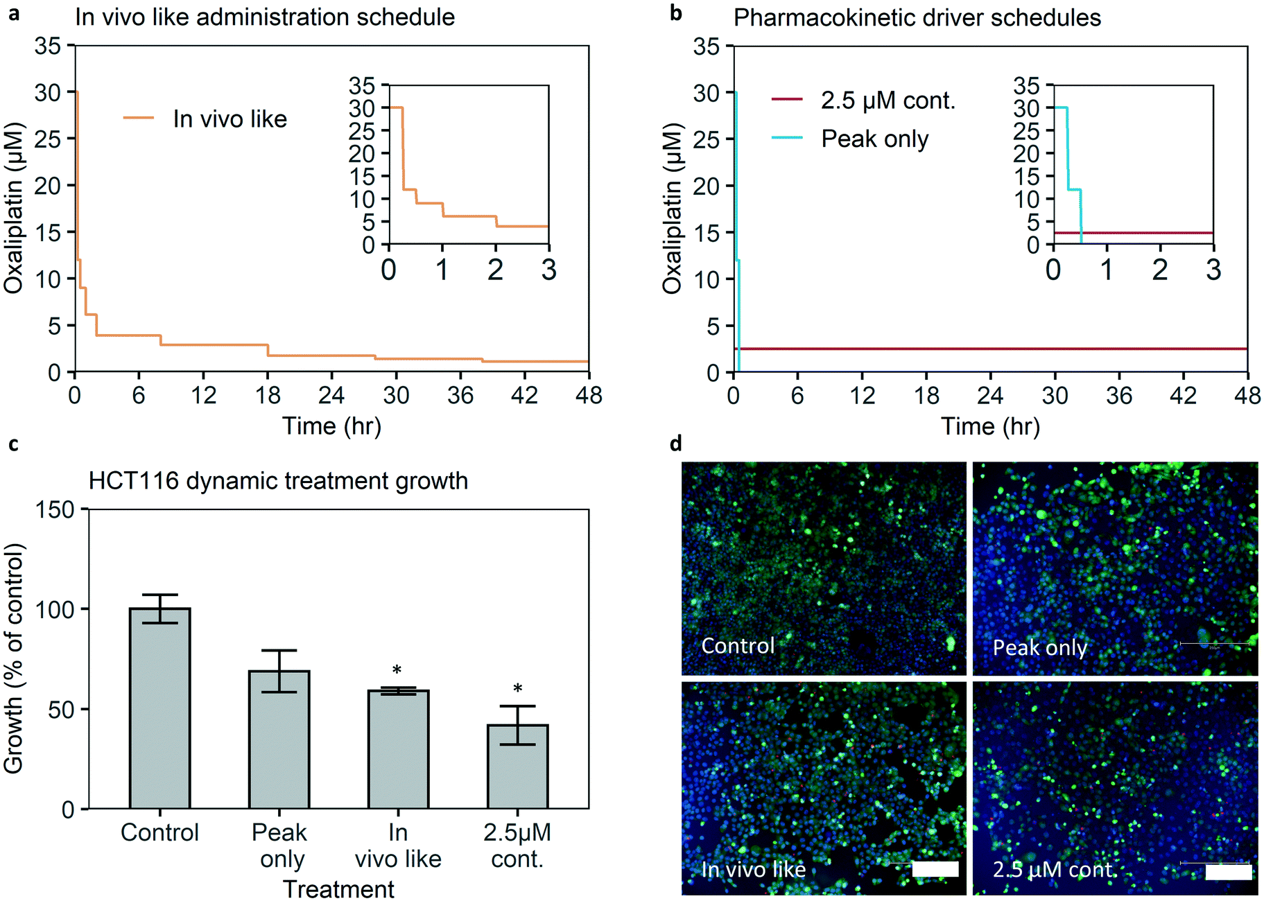

Fig. 5 HCT116 growth under in vivo-like oxaliplatin concentrations and pharmacokinetic driver exploration. (a) Administration schedule of the in vivo-like drug concentration over time. (b) Administration schedules for 2.5 μM oxaliplatin continuous, which leads to an equal AUC as the in vivo-like administration, and a peak only administration, which leads to an equal C_max as the in vivo-like administration. (c) Confluency growth of cells treated with dynamic drug concentrations. In vivo-like, oxaliplatin concentration growth is 60% of continuous medium perfusion (control). In vivo-like and 2.5 μM continuous have a significant lower growth than control, whereas peak only does not. N = 3–5 per treatment condition, n = 8 for control. Error bars are SEM. *p < 0.05 versus control growth. (d) Staining shows mostly live cells, with limited late-stage apoptosis for the in vivo-like exposure. Cell nuclei (NucBlue/Hoechst 33342, blue), viability (calcein AM, green), late stage apoptosis (ethidium homodimer, red). Scale bar 200 μm.

Using concentration profiles to find the pharmacokinetic driver of efficacy of oxaliplatin

The dynamic control over drug concentrations that our system provides can be used to perform detailed studies on the role of pharmacokinetic parameters in drug efficacy. For example, to our knowledge, it is not experimentally verified whether the peak concentration (C_max) is the major driver of efficacy of oxaliplatin, or whether continuous exposure to the average in vivo concentration over 48 hours would lead to higher growth inhibition.

To investigate whether the C_max or continuous exposure is more effective we compare the efficacy of two treatment schedules: one without a peak but with the average in vivo concentration of 2.5 μM over 48 hours. This concentration results in an area under the curve (AUC) equal to the AUC of the in vivo concentration profile of 120 μM h. And the second schedule with only the peak exposure but without (90% of) the AUC, i.e. after the first 30 minutes of the in vivo-like administration schedule containing the 30 μM (administration) peak, 47.5 hours of medium perfusion (Fig. 5d).

When 2.5 μM oxaliplatin is continuously administered, confluency growth is 40% of control, with a statistically significant difference versus control growth. If peak exposure only is administered cell growth is higher at 70% of control, and the difference versus control growth is not statistically significant. This implies continuous exposure is a more important pharmacokinetic driver of efficacy than peak exposure in our model. Retaining or even improving efficacy with constant exposure without a peak could be relevant for drug dose schedule optimization, as clinical experience suggests prolonging oxaliplatin infusion time from 2 to 6 hours reduces side effects.⁹

A potential explanation for efficacy improvement through constant exposure could be the time needed for oxaliplatin to enter the cell and exert its main effect through binding to DNA at sufficient levels. Transport across membranes and DNA binding can be relatively slow, as time to equilibrium intracellular concentration could take as much as 24 hours at a stable extracellular concentration for HCT116 cells.^44,45 When peak exposure is very short compared to time needed for equilibrium, as is the case for a 30 minute peak versus a 24 hour equilibrium, achieved DNA bound oxaliplatin will be relatively low. Growth inhibition will then be low as well, if peak DNA bound oxaliplatin determines growth inhibition, as is suggested for cisplatin.⁷ However shorter equilibrium times have been found for other cell lines,⁴⁶ which could lead to a higher effect of a peak exposure. Furthermore potential off-target (desired) effects could also change the relative contribution of peak and continuous exposure, especially if the pharmacokinetic–pharmacodynamic relation is different for on-target and off-target binding.

Hence for guiding drug schedule optimization, e.g. bolus versus extended infusion times, several in vitro and in silico models should ideally be combined in a single study. Besides combining these assays, the chip system could incorporate other potentially relevant biological factors. Administered dosages could be corrected for in vivo protein binding as drug effectiveness is likely caused by free drug concentrations.⁴⁷ Also the cell chamber can be adjusted to mimic the tumour microenvironment. E.g. by introducing different cell types, 3D structures and nutrient variation. By leveraging recent advances in organ-on-chip and cancer-on-chip technology, the in vitro–in vivo gap can be further reduced.⁴⁸

Conclusions

In this study we have administered a dynamic, in vivo-like, drug concentration of first line drug oxaliplatin to colorectal cancer cells in a microfluidic device. Growth (inhibition) was measured label free on chip. We found significant growth inhibition of oxaliplatin at an in vivo-like dose, primarily driven by continuous exposure and not maximum concentration (C_max). Hence microfluidics, with its ability to control geometries, flow and concentrations, enables mimicking in vivo-like drug concentrations in cell culture experiments. This is an emerging field in microfluidics.^{14,15,20–23} We contribute to this emerging field by offering an alternative technology to induce and validate dynamic dosing, test a drug used in the clinic, and translate clinical pharmacokinetics to technical requirements. We foresee use of this technology in the drug discovery process, for example in the lead optimization process where a handful of drugs are tested and optimized in in vitro and in vivo models. The device could aide in optimization and selection of compounds, based on pharmacokinetics found in mice. In the device also additional cell lines and concentration profiles could be tested. In general, the described microfluidic technology could be used for (i) increasing the mechanistic and predictive translational quality of in vitro models, including advanced microfluidic organ-on-a-chip and cancer-on-chip models,^17,48,49 (ii) finding the pharmacokinetic driver of efficacy and optimizing dosing strategies, and (iii) screening and selection of novel and repurposing drugs.

Contributions

J. K. – conceptualization, formal analysis, investigation, methodology, validation, visualization, writing – original draft; E. Y. W. – formal analysis, investigation, methodology; R. W. K. – formal analysis, investigation, methodology; J. R. – investigation; C. L. – formal analysis, methodology, resources, investigation; A. B. – conceptualization, funding acquisition, resources, supervision, writing – review & editing; A. D. M. – conceptualization, methodology, supervision, visualization, writing – review & editing.

Conflicts of interest

There are no conflicts to declare.

Acknowledgements

The authors acknowledge the funding received from the Dutch Science Foundation (NWO) under the Gravitation Grant “NOCI” Program (Grant No. 024.003.001) and the MESA+ Sensing Program.

Notes and references

1. Cancer diagnosis and treatment statistics, https://www.cancerresearchuk.org/health-professional/cancer-statistics/diagnosis-and-treatment#heading-Five, (accessed 10/03/2020).
2. S. Li, Y. Chen, S. Zhang, S. S. More, X. Huang and K. M. Giacomini, Pharm. Res., 2011, 28, 610–625.
3. Y. Ji, J. Y. Jin, D. M. Hyman, G. Kim and A. Suri, Clin. Transl. Sci., 2018, 11, 345–351.
4. NCI-60 Screening Methodology, https://dtp.cancer.gov/discovery_development/nci-60/methodology.htm, (accessed 10/03/2020).
5. A. Eastman, Oncotarget, 2017, 8, 8854–8866.
6. D. R. Liston and M. Davis, Clin. Cancer Res., 2017, 23, 3489–3498.
7. A. W. El-Kareh and T. W. Secomb, Neoplasia, 2003, 5, 161–169.
8. N. L. Jumbe, Y. Xin, D. D. Leipold, L. Crocker, D. Dugger, E. Mai, M. X. Sliwkowski, P. J. Fielder and J. Tibbitts, J. Pharmacokinet. Pharmacodyn., 2010, 37, 221–242.
9. S. Brienza, M. A. Bensmaine, P. Soulie, C. Louvet, E. Gamelin, E. Francois, M. Ducreux, M. Marty, T. Andre, F. de Braud, H. Bleiberg, V. Segal, M. Itzhaki and E. Cvitkovic, Ann. Oncol., 1999, 10, 1311–1316.
10. E. Van Cutsem, A. Cervantes, R. Adam, A. Sobrero, J. H. Van Krieken, D. Aderka, E. A. Aguilar, A. Bardelli, A. Benson, G. Bodoky, F. Ciardiello, A. D'Hoore, E. Diaz-Rubio, J. Y. Douillard, M. Ducreux, A. Falcone, A. Grothey, T. Gruenberger, K. Haustermans, V. Heinemann, P. Hoff, C. H. Kohne, R. Labianca, P. Laurent-Puig, B. Ma, T. Maughan, K. Muro, N. Normanno, P. Osterlund, W. J. Oyen, D. Papamichael, G. Pentheroudakis, P. Pfeiffer, T. J. Price, C. Punt, J. Ricke, A. Roth, R. Salazar, W. Scheithauer, H. J. Schmoll, J. Tabernero, J. Taieb, S. Tejpar, H. Wasan, T. Yoshino, A. Zaanan and D. Arnold, Ann. Oncol., 2016, 27, 1386–1422.
11. N. Isoherranen, R. Madabushi and S. M. Huang, Clin. Transl. Sci., 2019, 12, 113–121.
12. P. K. Vaddady, R. E. Lee and B. Meibohm, Future Med. Chem., 2010, 2, 1355–1369.
13. A. D. van der Meer and A. van den Berg, Integr. Biol., 2012, 4, 461–470.
14. S. Kim, S. C. LesherPerez, B. C. Kim, C. Yamanishi, J. M. Labuz, B. Leung and S. Takayama, Biofabrication, 2016, 8, 015021.
15. S. Y. Lockwood, J. E. Meisel, F. J. Monsma Jr. and D. M. Spence, Anal. Chem., 2016, 88, 1864–1870.
16. A. Valero, F. Merino, F. Wolbers, R. Luttge, I. Vermes, H. Andersson and A. van den Berg, Lab Chip, 2005, 5, 49–55.
17. K. P. Valente, S. Khetani, A. R. Kolahchi, A. Sanati-Nezhad, A. Suleman and M. Akbari, Drug Discovery Today, 2017, 22, 1654–1670.
18. F. Eduati, R. Utharala, D. Madhavan, U. P. Neumann, T. Longerich, T. Cramer, J. Saez-Rodriguez and C. A. Merten, Nat. Commun., 2018, 9, 2434.
19. J. Komen, F. Wolbers, H. R. Franke, H. Andersson, I. Vermes and A. van den Berg, Biomed. Microdevices, 2008, 10, 727–737.
20. C. Lohasz, O. Frey, F. Bonanini, K. Renggli and A. Hierlemann, Front. Bioeng. Biotechnol., 2019, 7, 72.
21. D. B. Chou, V. Frismantas, Y. Milton, R. David, P. Pop-Damkov, D. Ferguson, A. MacDonald, O. Vargel Bolukbasi, C. E. Joyce, L. S. Moreira Teixeira, A. Rech, A. Jiang, E. Calamari, S. Jalili-Firoozinezhad, B. A. Furlong, L. R. O'Sullivan, C. F. Ng, Y. Choe, S. Marquez, K. C. Myers, O. K. Weinberg, R. P. Hasserjian, R. Novak, O. Levy, R. Prantil-Baun, C. D. Novina, A. Shimamura, L. Ewart and D. E. Ingber, Nat. Biomed. Eng., 2020, 4(4), 394–406.
22. Y. A. Guerrero, D. Desai, C. Sullivan, E. Kindt, M. E. Spilker, T. S. Maurer, D. E. Solomon and D. W. Bartlett, AAPS J., 2020, 22, 53.
23. P. Golby, E. Buffa, T. Kostrzewski and D. Hughes, Cancer Res., 2018, 78, LB-044.
24. T. Stylianopoulos, L. L. Munn and R. K. Jain, Trends Cancer, 2018, 4, 292–319.
25. J. Schindelin, I. Arganda-Carreras, E. Frise, V. Kaynig, M. Longair, T. Pietzsch, S. Preibisch, C. Rueden, S. Saalfeld, B. Schmid, J. Y. Tinevez, D. J. White, V. Hartenstein, K. Eliceiri, P. Tomancak and A. Cardona, Nat. Methods, 2012, 9, 676–682.
26. M. W. Toepke and D. J. Beebe, Lab Chip, 2006, 6, 1484–1486.
27. T. Casalini, M. Salvalaglio, G. Perale, M. Masi and C. Cavallotti, J. Phys. Chem. B, 2011, 115, 12896–12904.
28. S. Modok, R. Scott, R. A. Alderden, M. D. Hall, H. R. Mellor, S. Bohic, T. Roose, T. W. Hambley and R. Callaghan, Br. J. Cancer, 2007, 97, 194–200.
29. Y. Ning, M. J. Labonte, W. Zhang, P. O. Bohanes, A. Gerger, D. Yang, L. Benhaim, D. Paez, D. O. Rosenberg, K. C. Nagulapalli Venkata, S. G. Louie, N. A. Petasis, R. D. Ladner and H. J. Lenz, Mol. Cancer Ther., 2012, 11, 1353–1364.
30. G. P. Nagaraju, O. B. Alese, J. Landry, R. Diaz and B. F. El-Rayes, Oncotarget, 2014, 5, 9980–9991.
31. K. Xu, G. Chen, Y. Qiu, Z. Yuan, H. Li, X. Yuan, J. Sun, J. Xu, X. Liang and P. Yin, Oncotarget, 2017, 8, 21719–21732.
32. N. Jaccard, L. D. Griffin, A. Keser, R. J. Macown, A. Super, F. S. Veraitch and N. Szita, Biotechnol. Bioeng., 2014, 111, 504–517.
33. S. Preibisch, S. Saalfeld and P. Tomancak, Bioinformatics, 2009, 25, 1463–1465.
34. E. W. Young and D. J. Beebe, Chem. Soc. Rev., 2010, 39, 1036–1048.
35. J. D. Wang, N. J. Douville, S. Takayama and M. ElSayed, Ann. Biomed. Eng., 2012, 40, 1862–1873.
36. A. W. Auner, K. M. Tasneem, D. A. Markov, L. J. McCawley and M. S. Hutson, Lab Chip, 2019, 19, 864–874.
37. Oxaliplatin, https://www.drugbank.ca/drugs/DB00526, (accessed 10/03/2020).
38. A. M. Hosios, V. C. Hecht, L. V. Danai, M. O. Johnson, J. C. Rathmell, M. L. Steinhauser, S. R. Manalis and M. G. Vander Heiden, Dev. Cell, 2016, 36, 540–549.
39. M. A. Graham, G. F. Lockwood, D. Greenslade, S. Brienza, M. Bayssas and E. Gamelin, Clin. Cancer Res., 2000, 6, 1205–1218.
40. M. P. di Cagno, F. Clarelli, J. Våbenø, C. Lesley, S. D. Rahman, J. Cauzzo, E. Franceschinis, N. Realdon and P. C. Stein, Mol. Pharmaceutics, 2018, 15, 1488–1494.
41. A. L. Paguirigan and D. J. Beebe, Integr. Biol., 2009, 1, 182–195.
42. A. Single, H. Beetham, B. J. Telford, P. Guilford and A. Chen, J. Biomol. Screening, 2015, 20, 1286–1293.
43. K. Kay, K. Dolcy, R. Bies and D. K. Shah, AAPS J., 2019, 21, 27.
44. N. Kitada, K. Takara, T. Minegaki, C. Itoh, M. Tsujimoto, T. Sakaeda and T. Yokoyama, Cancer Chemother. Pharmacol., 2008, 62, 577–584.
45. T. Tippayamontri, R. Kotb, B. Paquette and L. Sanche, Invest. New Drugs, 2011, 29, 1321–1327.
46. A. Ghezzi, M. Aceto, C. Cassino, E. Gabano and D. Osella, J. Inorg. Biochem., 2004, 98, 73–78.
47. J. Heuberger, S. Schmidt and H. Derendorf, J. Pharm. Sci., 2013, 102, 3458–3467.
48. S. N. Bhatia and D. E. Ingber, Nat. Biotechnol., 2014, 32, 760–772.
49. A. van den Berg, C. L. Mummery, R. Passier and A. D. van der Meer, Lab Chip, 2019, 19, 198–205.

---

Footnote

† Electronic supplementary information (ESI) available. See DOI: 10.1039/d0lc00419g

---