
 Open Access Article
 This Open Access Article is licensed under a Creative Commons Attribution-Non Commercial 3.0 Unported Licence
Multidimensional protein characterisation using microfluidic post-column analysis†
Tom
Scheidt‡
 a,
Tadas
Kartanas‡
a,
Quentin
Peter
ab,
Matthias M.
Schneider
a,
Kadi L.
Saar
a,
Thomas
Müller
b,
Pavan Kumar
Challa
a,
Aviad
Levin
a,
Sean
Devenish
b and
Tuomas P. J.
Knowles
*ac
a,
Tadas
Kartanas‡
a,
Quentin
Peter
ab,
Matthias M.
Schneider
a,
Kadi L.
Saar
a,
Thomas
Müller
b,
Pavan Kumar
Challa
a,
Aviad
Levin
a,
Sean
Devenish
b and
Tuomas P. J.
Knowles
*ac
aCentre for Misfolding Diseases, Department of Chemistry, University of Cambridge, Lensfield Road, Cambridge CB2 1EW, UK. E-mail: tpjk2@cam.ac.uk
bFluidic Analytics Ltd, Unit A, The Paddocks Business Centre, Cherry Hinton Rd, Cambridge CB1 8DH, UK
cCavendish Laboratory, Department of Physics, University of Cambridge, J J Thomson Avenue, Cambridge CB3 0HE, UK
First published on 26th June 2020
Abstract
The biological function of proteins is dictated by the formation of supra-molecular complexes that act as the basic machinery of the cell. As such, measuring the properties of protein species in heterogeneous mixtures is of key importance for understanding the molecular basis of biological function. Here, we describe the combination of analytical microfluidic tools with liquid chromatography for multidimensional characterisation of biomolecules in complex mixtures in the solution phase. Following chromatographic separation, a small fraction of the flow-through is distributed to multiple microfluidic devices for analysis. The microfluidic device developed here allows the simultaneous determination of the hydrodynamic radius, electrophoretic mobility, effective molecular charge and isoelectric point of isolated protein species. We demonstrate the operation principle of this approach with a mixture of three unlabelled model proteins varying in size and charge. We further extend the analytical potential of the presented approach by analysing a mixture of interacting streptavidin with biotinylated BSA and fluorophores, which form a mixture of stable complexes with diverse biophysical properties and stoichiometries. The presented microfluidic device positioned in-line with liquid chromatography presents an advanced tool for characterising multidimensional physical properties of proteins in biological samples to further understand the assembly/disassembly mechanism of proteins and the nature of complex mixtures.
Introduction
The formation of discrete structures by proteins is dictated by their ability to correctly fold, interact and assemble into hierarchically ordered complexes. Thus, the ability of proteins to serve as the basic machinery in cells is governed by their range of static and dynamic interactions enabling their flexible and specific functionality. Therefore, it is not surprising that over 80% of proteins do not appear on their own, but as part of complexes.1 The nature of these interactions is defined by the specific amino acid sequences of the proteins and their post-translational modifications,2 thus modulating their interactions.3–6 In particular, the direct electrostatic interactions are enabled by charged and polar groups at the protein surface that allow the formation of ion pairs, hydrogen bonds and other electrostatic interactions. The overall protein charge and formation of complexes in solution are dependent on the number and nature of the charged groups presented and is related to the isoelectric point (pI), known as the pH value at which the net charge is zero.7 While electrostatic interactions can be highly specific and possess strong geometric constraints, hydrophobic interactions minimise water-exposed hydrophobic residues, and these are usually buried inside proteins or protein complexes.8 Malfunctioning proteins that misfold and interact in an unregulated manner can lead to protein aggregation, a key feature in many neurodegenerative diseases. Thus, this wide range of interactions is a key feature of protein self-assembly and function, both in vivo and in vitro.Techniques capable of characterising complex mixtures are limited and commonly only allow to determine unidimensional information. As protein complexes are highly dynamic and their composition is dependent on exogenous factors including temperature, pH, local salt concentration and viscosity, it is challenging to determine their biophysical properties under physiological conditions. Simultaneous acquisition of multidimensional characteristics is therefore essential as state and compositions of the sample can change between sequential measurements. Conventional approaches for multidimensional characterisation include e.g. size exclusion chromatography coupled to multi-angle light scattering (SEC-MALS),9 2D-gel electrophoresis,10 liquid chromatography-mass spectrometry (LC-MS),11 LC coupled to nuclear magnetic resonance spectroscopy (LC-NMR),12 high performance anion exchange coupled with pulsed amperometric detection (HPAEC-PAD)13 and electrochromatography.14,15 In many cases, these approaches require special probes, including isotopes, oxidisable functional groups, protein tags or fluorescence labeling13,16 or the use non-physiological conditions, such as sample ionisation and high sample concentration.17 The difficulty in conserving protein conformation and observing non-native complexes, can in principle, be avoided by operating under physiological conditions. Yet, methods with high separation power that work under these conditions have been found challenging to develop and adapt.
In order to overcome current challenges in obtaining high resolution understanding caused by the diversity of molecular species of heterogeneous samples, most of the techniques described above have a chromatographic and/or electrophoretic step as part of the workflow, which requires large sample volumes. The stationary phase used in chromatography can have a major influence on the purification strategy and can consist of biomolecules such as dextran, agarose or cellulose or synthetic substrate such as polyacrylamide, polystyrene or silica-based polymers.18 By contrast, the selection of the mobile phase controls the interplay between the analyte molecules and the matrix and is usually organic or buffered.19
Microfluidic systems are used to parallelise different assays while allowing small sample volumes being used. Such lab-on-a-chip devices enable manipulation and control over small quantities of fluids, usually in the range of pico- to microliters.20 Examples of microfluidic analytical tools are diffusional sizing,21–24 capillary electrophoresis,25 free-flow electrophoresis (FFE)26–30 and microscale thermophoresis.31,32 Along with the wide range of existing LC methods, e.g. size exclusion, reversed phase, ion-exchange and affinity chromatography,21,33–37 microfluidic tools can be used for a resolved characterisation of physiological protein complexes from endogenous samples.38,39
In this study, we combine high flow size exclusion chromatography with microfluidic protein analysis. A small fraction of the eluting sample was continuously distributed between two functionally separate fluidic circuits. By measuring the sample composition in the condensed phase, we were able to analyse proteins and their complex formation under native conditions. The microfluidic systems applied here allow for the simultaneous determination of hydrodynamic radius and electrophoretic mobility of molecules in a quantitative manner in complex mixtures.23,24,27,29,40 Furthermore, by applying multiple orthogonal downstream analyses approaches, we were able to increase the limited effective resolution of the SEC column. In order to quantify multiple biophysical parameters, the individual microfluidic components were arranged to fit within a single camera field of view (Fig. 2b), where one part documents the deflection of molecules in an electric field applied on an electrophoretic chamber (Fig. 2c) and a second part records the molecular diffusion at distinct positions along a channel. The acquired intensity of the diffused molecules in converted into two-dimensional profiles and fitted against theoretical basis functions assuming a range of hydrodynamic radii (Fig. 2a). Only a small fraction of the solution is used for analysis, whereas the main volume of the sample is collected and can be used for further evaluation.
Materials and methods
Analyte mixtures
To demonstrate the functionality of the method for the characterisation of model proteins, we selected a mixture of three proteins varying in size and pI: bovine thyroglobulin (MW = 670 kDa, pI = 4.5, GE Healthcare, 28-4038-42), chicken conalbumin (MW = 76 kDa, pI = 6.7, GE Healthcare, 28-4038-42,) and chicken lysozyme (MW = 14.3 kDa, pI = 9.3, Sigma-Aldrich, L6876) (Fig. S1a†). The proteins were diluted in a 100 mM sodium HEPES buffer (pH 7.3) to a concentration of 4.6, 33 and 110 μM, respectively; total sample volume was 40 μL.We further used a second system to generate a heterogeneous sample, which was based on streptavidin–biotin complex formation. This mixture was prepared by incubating streptavidin (Prospec, Israel, PRO-791), biotinylated bovine serum albumin (Generon, UK, 7097-5) and biotinylated Atto488 dye (ATTO-TEC GmbH, Germany) at concentrations of 15.7, 15.7 and 47.1 μM, respectively (total volume 50 μL), for 1 h at room temperature in 10% phosphate buffered saline (0.1× PBS) at pH 6.5, 7.3 and 8.2. The mixture is expected to form seven distinct complexes with masses ranging from 1 kDa to 300 kDa (Fig. S1b†). Five of the complexes contain an Atto488 fluorophore and, therefore, the latter molecules were the focus of detection and analysis.
LC separation
Two different buffers were used for the elution of the sample through the column. First, we used a 100 mM sodium HEPES buffer (pH 7.3) for the label-free sample characterisation. In contrast, the streptavidin–biotin mixture was eluted in a 0.1× PBS buffer with a pH of either 6.5, 7.3 or 8.2. Both buffers also contained 0.01% sodium azide and 0.1% Tween to reduce sample adhesion to microfluidic channels. A Superdex 200 Increase 3.2/300 column (GE Healthcare, UK) at a flow rate of 600 μL h−1 was operated on an ÄKTA Pure System (GE Healthcare, UK). Eluting sample absorption at 280 nm and 500 nm wavelengths were monitored simultaneously using a 10 mm path length absorption monitor U9-M (GE Healthcare, UK). The absorption intensity was used for matching the molecular elution volume with the image sequence on a fluorescence microscope. The flow from the LC separation was connected to the microfluidic flow adapter.Microfluidic flow adapter
A microfluidic junction (P-722, IDEX Health & Science, USA) with carefully pre-cut polyether ether ketone (PEEK) capillaries (IDEX Health & Science, USA) and two flow sensors (MF2 420 μL h−1, Elveflow, France) was designed and fabricated, directing only a fraction of the flow which eluted from chromatographic separation into individual parts of the microfluidic device (Fig. S2 and S6†). The lengths of the capillaries were as follows: the flow adapter has three outlets (Fig. S6†). One fractionator output was fabricated of a capillary with Lf = 10.2 cm and 125 μm ID and the outputs A and B were made of two capillaries with L1 = 10 cm with 125 μm ID each leading to individual flow sensors, each followed by a capillary with L2 = 8.1 cm with 67.8 μm ID. Both capillaries were connected to a microfluidic device operating at flow rates close to few 100 μL h−1 (∼102 μL h−1). In general, the flow from the LC protein separation can be in the range of 600 μL h−1–60 mL h−1 (600 μL h−1–60 ml h−1), depending on the pressure and column used. The individual flow rates leaving the flow splitter were set by the individual capillary resistances. The flow sensors were integrated into the ÄKTA Pure system with an I/O-box E9 for real time flow monitoring (GE Healthcare, UK). Stable flow splitting was achieved, directing ∼10% of the total flow to different areas of the microfluidic chip (Fig. S3†). The flow rates at the diffusional sizing and the electrophoresis device sample inlets were measured to be 40.0 ± 0.7 μL h−1 and 37.4 ± 0.7 μL h−1, respectively.Flow control
The need for purification or separation techniques of complex mixtures in biomolecular studies is vast. However, most of these bulk techniques cannot directly be transferred to microfluidic scales due to the high pressure flow systems commonly used. In order to match macrofluidic flows used in chromatographic systems with microfluidic flows found in chips with micron sized features, a flow adapter scalable to a wide range of rates had to be designed and implemented (Fig. 1). The incoming flow can be split into numerous outlets, each adjusted for specific applications. Thus, our flow adapter interface enables a standard LC separation, followed by simultaneous multidimensional characterisation. The LC system used was an ÄKTA Pure system which drives two high pressure pumps maintaining a highly stable flow with a 1–5% fluctuation level depending on the buffer and the separation column used (Fig. S3†). In our experiments, the microfluidic flow adapter with carefully adjusted resistances distributed the fluid from the LC absorption measurement cell between two microfluidic sample inlets and a fractionation outlet. The flow rates at the chip inlets for the free-flow electrophoresis and diffusional sizing were measured to be 6.7 ± 0.1% and 6.2 ± 0.1%, of the initial flow rate, respectively. The rest of the post LC separation fluid not used for further characterisation (∼90%) was collected via the fractionation outlet. The ratios used were adapted to the microfluidic application used or separation procedure applied.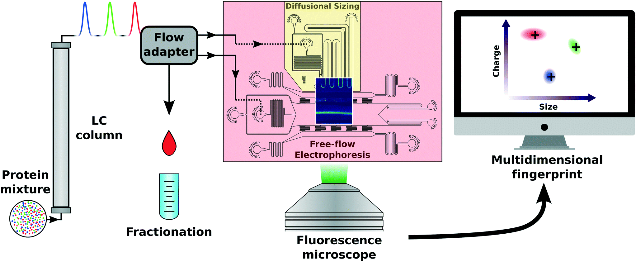 | ||
| Fig. 1 Scheme of liquid chromatography with integrated (in-line) analytical microfluidics. Starting with a complex protein mixture, the molecules are separated by their individual properties depending on the column applied. The eluting liquid is divided by a macro- to microfluidic flow adapter. Following this step, the flow-through can be guided to individual microfluidic components or collected separately. In this way, the hydrodynamic radius and electrophoretic mobility of the eluted species can be measured continuously using a microfluidic chip. The acquired information is processed to generate multidimensional information of individual species in a complex mixture. | ||
Microfluidic chip fabrication
The devices were fabricated using standard polydimethylsiloxane (PDMS) through soft-lithography approaches as have been previously described.41 The master for the replica molding of PDMS was fabricated with an SU-8 photolithography process.42 After mixing PDMS (Sylgard184, Dow Corning, two components 10![[thin space (1/6-em)]](https://www.rsc.org/images/entities/char_2009.gif) :1 ratio and degassed) and casting it onto the photo-lithographically defined structure, it was cured at 65 °C for 1 h. A carbon black nanopowder, <100 nm particle size (Sigma-Aldrich, 633100), was added to the PDMS before curing to generate black devices (see Fig. S8†), thus minimising background noise and the unwanted autofluorescence from PDMS under 280 nm-LED illumination during the measurements as have been previously shown.40 The PDMS replica of each master was then cut, and the connection holes were generated using a biopsy punch. The PDMS device was sonicated for 3 min in isopropanol, blow-dried with N2, and placed in an oven at 65 °C for 10 min. Finally, the replica was activated using O2 plasma at a 40% power for 10 s (Diener etcher Femto, Germany) and bonded to a clean quartz slide (Alfa Aesar, 76.2 × 25.4 × 1.0 mm) for UV measurements or a simple glass slide for fluorescence measurements.
:1 ratio and degassed) and casting it onto the photo-lithographically defined structure, it was cured at 65 °C for 1 h. A carbon black nanopowder, <100 nm particle size (Sigma-Aldrich, 633100), was added to the PDMS before curing to generate black devices (see Fig. S8†), thus minimising background noise and the unwanted autofluorescence from PDMS under 280 nm-LED illumination during the measurements as have been previously shown.40 The PDMS replica of each master was then cut, and the connection holes were generated using a biopsy punch. The PDMS device was sonicated for 3 min in isopropanol, blow-dried with N2, and placed in an oven at 65 °C for 10 min. Finally, the replica was activated using O2 plasma at a 40% power for 10 s (Diener etcher Femto, Germany) and bonded to a clean quartz slide (Alfa Aesar, 76.2 × 25.4 × 1.0 mm) for UV measurements or a simple glass slide for fluorescence measurements.
Microfluidic chip design and operation
The microfluidic chip was designed to fit two distinct analytical areas in one fluorescence microscope field of view (Fig. 2b), a diffusional sizing and a free-flow electrophoresis part. The diffusional sizing part consists of a long diffusion channel of a length of LD = 43 mm, a width of WD = 200 μm and a height of HD = 55 μm (Fig. 1 and 2b). The positions for diffusion profile acquisition were chosen to allow a high dynamic range for sizing and have been fixed at distances of 1.4 mm, 2.0 mm, 10.7 mm, 11.3 mm, 19.9 mm, 20.5 mm and 39.2 mm from the sample injection point. A degassed co-flow buffer (same as the LC mobile phase) was injected at a 150 μL h−1 flow rate using a neMESYS syringe pump (CETONI GmbH, Germany). The outlet of one flow adapter was connected to the sample inlet on the diffusional sizing device. The injected sample diffusion profile was recorded and fitted to the numerical diffusion simulations (example shown in Fig. 2a).24,43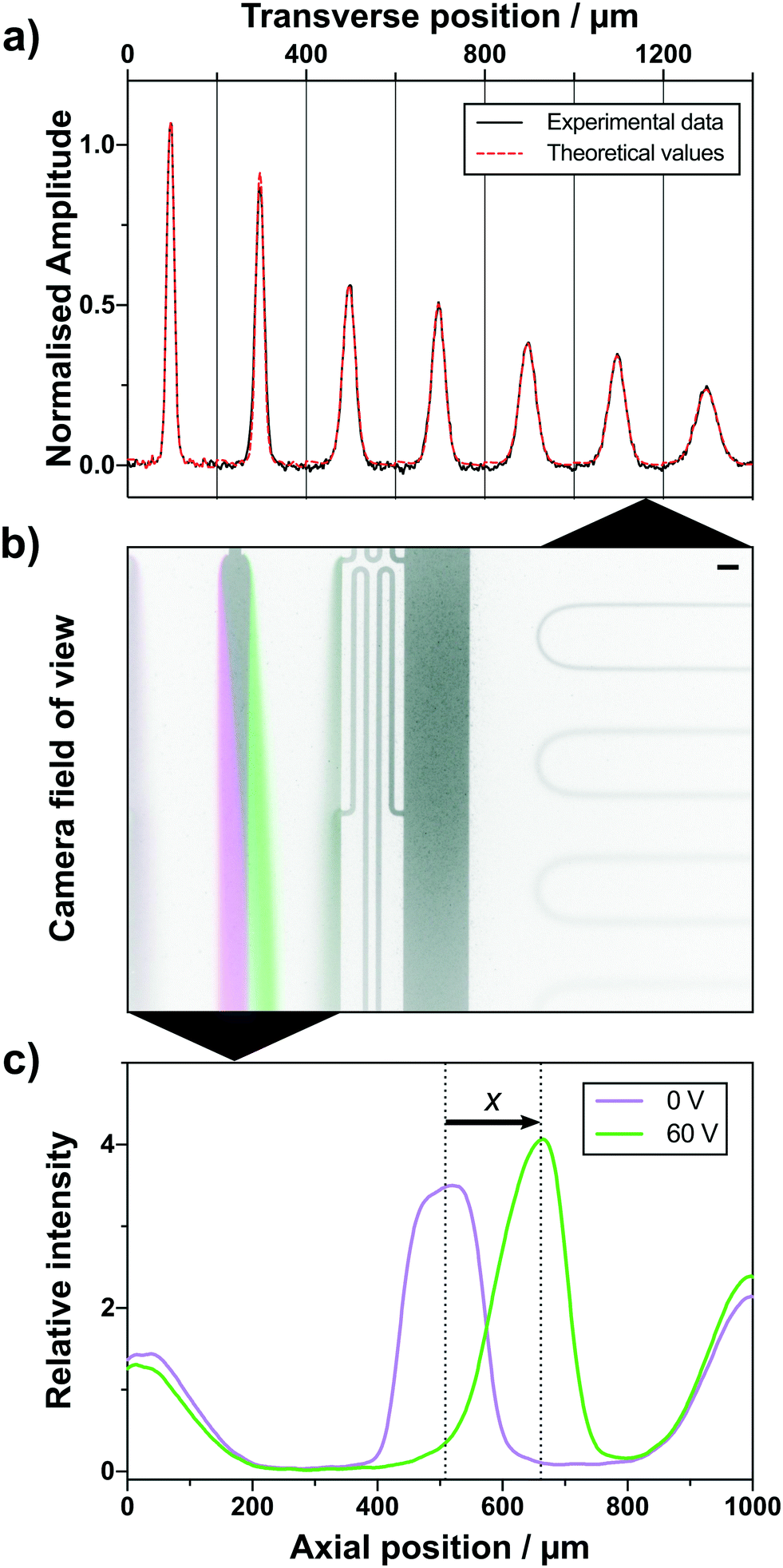 | ||
| Fig. 2 Microfluidic components in a single camera field of view with subsequent analytical processes. a) Experimental diffusion profiles (black curve) from the diffusional sizing are of the camera field of view (b) were fitted against theoretical basis functions (red dashed curve) resulting in a hydrodynamic radius prediction. b) Overlay of two images taken at 0 V (magenta) and 60 V (green). The field of view captures the microfluidic electrophoresis device on the left side and the diffusional sizing part on the right side. Scale bar represents 100 μm. c) The sample is deflected when an electric field of 60 V (green curve) is applied in the electrophoresis device. From the distance of deflection, x, the electrophoretic mobility can be deduced. | ||
The second part of the microfluidic chip was a free-flow electrophoresis device with liquid electrodes.27 It was designed to create up to 60 V cm−1 transverse electric fields on-chip, while avoiding bubble formation and electrolysis product build-up. We injected a conductive 3 M KCl electrolyte solution from the sides (Fig. 1) at flow rates of 150 μL h−1. The sheath flow buffer was injected at 150 μL h−1 using a neMESYS syringe pump. The second output of our flow adapter was connected to the sample inlet of our free-flow electrophoresis device. To establish electrical contacts, hollow stainless steel 1.5 mm ID electrodes were inserted into the liquid electrode channels on the sides of the device and connected to a power supply (EA Elektro-Automatik 6230207, Germany). The power supply was connected to the chip via liquid electrodes and a multimeter (Agilent 34410A, USA) to record the current flowing through the circuit.
The combined microfluidic blocks were operated continuously for approximately 3–5 h without any flow adjustments. Epifluorescence microscopy images were taken with 10 s intervals. These images were analysed to give hydrodynamic radius, electrophoretic mobility and charge for every 3.3 μL of the eluent from the column while still fractionating 90% of the total volume.
Fluorescence microscope setups
Two different fluorescence microscopes were used for the experiments: an intrinsic fluorescence microscope for a label-free protein detection40 and a green epifluorescence measurement setup for labelled samples. Autofluorescence measurements of proteins containing aromatic amino acids were performed by illuminating with a 25 mW 280 nm LED (M280L3, Thorlabs, UK) through an excitation filter (FF01-280/20-25, Semrock, USA) centred at a λex = 280 nm and a dichroic mirror (FF310-Di01-25 × 36, Semrock, USA). The fluorescence from the sample was collected through an emission filter (FF01-357/44-25, Semrock, USA) centred at λem = 357 nm, and focused onto a EMCCD camera (Rolera EMC2, QImaging, Canada) with an exposure time of 4 s.The green epifluorescence microscope, optimised for the green fluorescent protein (GFP)/Alexa488 detection, consisted of a 490 nm LED (M490L4, Thorlabs, UK), an excitation filter at 482 ± 9 nm, a dichroic mirror (350–488 nm/502–950 nm) and an emission filter at 520 ± 14 nm (filter set MDF-GFP2, Thorlabs, UK). The microscope had an xyz stage for accurate chip positioning in the field of view of a 2.5× objective, and images were acquired with an exposure time of 1 s per frame using a CCD camera (Retiga R1, QImaging, USA). A raw background corrected fluorescence image of a sample under test is shown in Fig. 1 and 2b.
Electrophoresis device calibration and mobility analysis
We applied a voltage V0 to the electrodes of the electrophoresis device. First, we performed the mobility measurements while recording the current flowing through the circuit, I. The electrophoresis chamber was then primed with the conductive electrolyte solution, effectively shorting the chamber so that the chamber electric resistance can be neglected (Rch ≈ 0). Thus, the current, I0, could be measured while applying the same voltage, V0 (Fig. S5†), allowing the estimation of the electrode resistance, Relec. Then| V0 = I(Relec + Rch), | (1) |
| V0 = I0Relec, | (2) |
The voltage drop across the electrophoresis chamber could be expressed as:
| ⇒V = IRch = Relec(I0 − I) = V0(1 − I/I0). | (3) |
Distance along the direction of flow d∥ can be expressed as:
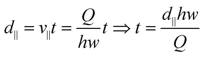 | (4) |
The mobility can be expressed as:
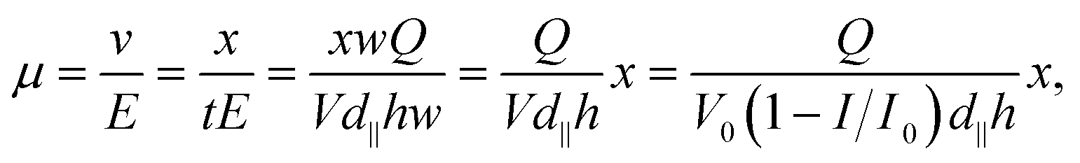 | (5) |
Size and charge calculation
The diffusion profiles were extracted by processing the images and removing the background using image alignment in the Fourier plane. The curve, generated by the non-uniform illumination intensity, was removed by multidimensional polynomial fitting. The channel edge positions and image rotation angle were detected and corrected automatically using an FFT-based technique.44 The noise was then reduced by spatial averaging along the channel before extracting the profiles at 7 predefined positions along the diffusion channel. Then, a set of basis functions, predicting the diffusion profiles of predefined sizes (diffusion coefficients), was generated.24,40,43,45 Finally, a fit deconvolving the measured experimental profiles into a linear combination of the simulated basis functions was computed using a least-squares error algorithm. The fit interpolation yielded the average eluting analyte hydrodynamic radius with the associated error.The measured hydrodynamic radius Rh and the electrophoretic mobility μe can be used to estimate the complex charge using the Nernst–Einstein relation:46
| q = Ze = 6πηRhμe, | (6) |
Isoelectric point prediction
The isoelectric point of BSA, streptavidin and their various combinations were predicted using the ExPASy online pI/Mw computing tool. Therefore, we used the sequence for BSA (UniProtKB P02769 [25-607]) and streptavidin (MAEAGITGTWYNQLGSTFIVTAGADGALTGTYESAVGNAESRYVLTGRYDSAPATDGSGTALGWTVAWKNNYRNAHSATTWSGQYVGGAEARINTQWLLTSGTTEANAWKSTLVGHDTFTKVKPSAAS).Results and discussion
Label-free protein characterisation
In order to examine whether this combined strategy allows for detecting and analysing a mixture of unlabelled proteins following SEC, we employed a UV-microscopy set up, capable of exciting aromatic amino acids and measuring their intrinsic fluorescence.40 Therefore, the sensitivity of our label free approach is dependent on the tryptophan and tyrosine composition of each protein. Previous studies have shown that the minimum content of tryptophan or tyrosine required for reliable detection using such microfluidic designs is ∼50 nM or 140 nM, respectively.40 The mixture used consisted of the three unlabelled proteins: thyroglobulin dimer (bovine), conalbumin (chicken) and lysozyme (chicken) (Fig. S1†). These proteins vary in mass from 14 to 670 kDa and were selected to give adequate separation by size exclusion chromatography. Therefore, the tested proteins were baseline separated into three major peaks eluting at volumes of 1.06 mL, 1.52 mL and 2.12 mL, respectively, with a minor conalbumin oligomer peak at 1.34 mL (Fig. 3). Following this, the eluting samples were continuously injected into a free-flow electrophoresis and diffusional sizing device (Fig. 1). More specifically, one fraction of the sample is loaded into an electrophoresis device between two liquid electrodes with a perpendicularly applied electric field. A second fraction of the sample is loaded into the diffusion device focused in the centre by a surrounding buffer co-flow geometry along a channel. The molecular diffusion is monitored in a time resolved manner by measuring at distinct position along the channel. Data from the two devices were combined to calculate the effective charge q of individual species (Fig. 3a–c). To determine the biophysical properties of the separated molecular species more accurately, we aligned the absorbance chromatogram measured using LC with the fluorescence intensity acquired on the microscope. The alignment is necessary to correlate intensity information of the chromatogram with the microfluidic based biophysical parameters acquired in series and, therefore, allows the specific assignment of individual species at a later stage. The measured signals of thyroglobulin, conalbumin and lysozyme correspond to hydrodynamic radii of 7.86 ± 0.30 nm, 3.96 ± 0.14 nm and 2.20 ± 0.14 nm, respectively (Fig. 3c). These measurements are in agreement with previously established values.47–49 Furthermore, we have been able to simultaneously acquire the effective charge of the components in the mixture as −19.4 ± 1.3, −0.8 ± 0.3 and 6.3 ± 0.4, corresponding to thyroglobulin, conalbumin and lysozyme, respectively (Fig. 3c). The measured net charge at pH 7.4 for the three analysed proteins correlates with previously reported pIs.50,51 We further analysed the measured information using a 3-D plot, showing molecular size vs. effective charge map with a 280 nm absorption intensity related color-map (Fig. 3b). The absorbance and therefore the third dimension is proportional to the relative abundance of detectable species and thus enables the identification of single species as bright spots in the 3-D plot. The plot shows three species with distinct biophysical properties. Thus, we demonstrate in-line label-free biophysical characterisation of a biomolecular mixture following SEC separation.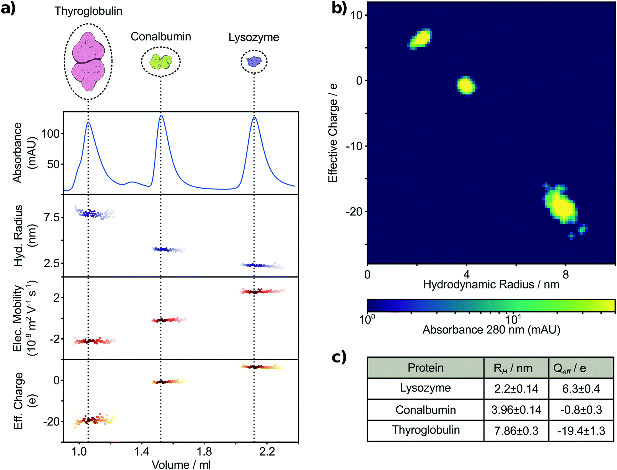 | ||
| Fig. 3 Label-free multidimensional characterisation of a ternary mixture of thyroglobulin, conalbumin and lysozyme by in-line SEC with parallel FFE and diffusional sizing. a) The mixture was separated by size exclusion chromatography into three major peaks and the eluting molecule size, electrophoretic mobility and effective charge were continuously measured. b) Individual measurements conducted every 20 s were analysed based on the molecular absorption at 280 nm revealing 3 major populations in the protein mixture with specific size and charge. c) Hydrodynamic radii and net charges of the three major peaks assigned to the proteins originally being used. | ||
Heterogeneous labelled analyte separation and characterisation
The advantage of fluorescent labels is an increase in sensitivity and specificity, such that detection of particular molecules is possible even in highly diverse mixtures and at low concentrations. Thus, fluorescent labeling enables tracking of individual interactions of a probe in complex solutions. In our study, we used a mixture of biotinylated BSA and biotinylated Atto488 dye, both capable of binding streptavidin with one of the strongest affinities found in nature (KD = 10−15 M).52 Using this approach, we observe a higher sensitivity when using Alexa488 labelled proteins by determining the fraction of the integrated intensity of the first detectable data point using fluorescent microscopy and the overall intensity of Alexa488 from the chromatogram. Thus, the lower limit of labelled protein detection for our application is ∼3 nM Alexa488. To illustrate the power of this technique and estimate yet another analytical dimension, we have repeated the experiment under three different pH conditions, 6.5, 7.3 and 8.2 and followed changes in molecular charges to investigate individual isoelectric points. In addition to the alignment of the absorbance intensity of the chromatogram with the biophysical parameter acquired using our microfluidic chip, we aligned the results of all three pH conditions for a better comparison of individual molecule properties. The LC separation of the Atto488 labelled streptavidin–biotin based system resulted in similar sample elution peaks for all three conditions (Fig. 4b). Simultaneously, we measured the size and electrophoretic mobility of the eluting material via fluorescence microscopy (see Materials and methods). Both sets of information were used to calculate the distinct net charge of each molecule (Fig. 4b). We plot the effective charge vs. molecular size where the intensity of each point is the absorption intensity at 500 nm, summarising the biophysical properties of the five Atto488 labelled molecular complexes abundant in the mixture (Fig. 4a). By further applying a Savitzky–Golay filter before and after taking the second derivative of the raw absorbance spectrum, four distinct Atto488 labelled molecules and the free dye itself can be assigned (Fig. S4a†). The first major peak with elution volume between 1 ml and 1.5 ml has three subpeaks which could not be separated completely due to the insufficient resolution at the given molecular weight range of our selected column. However, using our multiple orthogonal downstream analyses approach, we were able to increase the effective resolution of the SEC chromatogram. By applying the second derivative analysis of the absorption at 500 nm (Fig. S4a†) we estimated the approximate elution volumes for streptavidin with one, two and three BSA molecules to be 1.08 ml, 1.16 ml and 1.33 ml, respectively (Fig. S4b†). The second major peak with an elution volume between 1.5 ml and 1.9 ml can be identified as streptavidin with four Atto488 dye molecules and, finally, the last well-defined peak with an elution volume between 2 ml and 2.3 ml was the free biotinylated Atto488 dye. Furthermore, we have used the elution volume ranges to estimate the size and effective charge with the corresponding confidence intervals for each of those five species (Table 1). All molecules have a negative charge under the measured conditions and, more specifically, the charge of a biotinylated Atto488 dye was measured to be −1.00 ± 0.07 at pH 7.3 which agrees with the expected charge of −1.53 Streptavidin with four bound dyes resulted in a size of 3.21 ± 0.04 nm and an effective charge of −2.77 ± 0.12. The mono-, di-, and trivalent streptavidin–BSA complexes have hydrodynamic radii of 5.43 ± 0.07 nm, 7.39 ± 0.38 nm, 7.55 ± 0.92 nm and effective charges of −13.18 ± 0.51, −20.19 ± 1.20 and −23.19 ± 1.43 elementary charges, respectively (Table 1). The relative charge accumulation between each complex correlates with the relative amino acid contribution of the individual BSA/streptavidin components.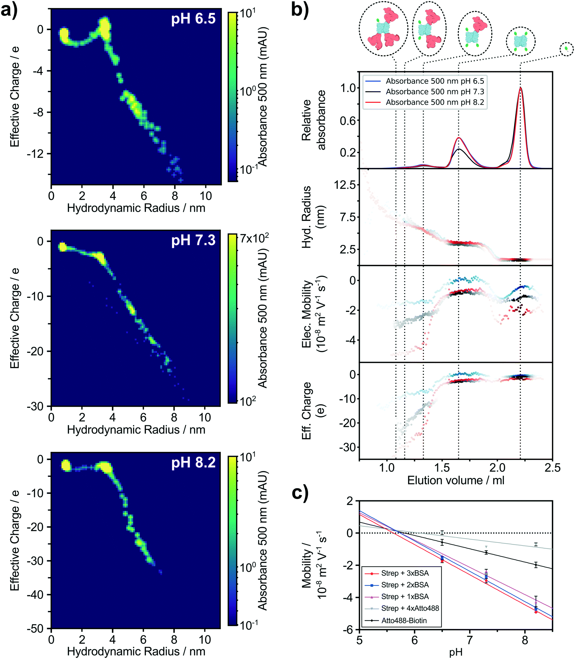 | ||
| Fig. 4 The labelled streptavidin/BSA/Atto488 mixture was characterised at three pH values. a) The five identified labelled molecule complexes were characterised and 3-dimensional charge vs. size maps were generated. The points are binned and weighted based on the absorption intensity at 500 nm. The third dimension given by the molecule absorbance at 500 nm is proportional to the detected protein labels and therefore bright spots can be related to individual species. b) The labelled mixture was incubated and separated via LC at pH 6.5 (blue curve and points), 7.3 (black curve and points) and 8.2 (red curve and points). The hydrodynamic radii, electrophoretic mobilities and effective charges of all elutions were recorded. c) Measured mobilities of the individual identified species were plotted against the different pH conditions and analysed further by linear regression. | ||
| Molecule | pH | R H/nM | Q eff/e | pItheo | pIexp |
|---|---|---|---|---|---|
| Atto488-biotin | 6.5 | 0.81 ± 0.01 | −0.44 ± 0.14 | — | 5.82 |
| 7.3 | 0.75 ± 0.01 | −1.00 ± 0.07 | |||
| 8.2 | 0.96 ± 0.02 | −1.79 ± 0.01 | |||
| Strep + 4xAtto488 | 6.5 | 3.47 ± 0.09 | 0.07 ± 0.40 | 6.09 | 6.10 |
| 7.3 | 3.21 ± 0.04 | −2.77 ± 0.12 | |||
| 8.2 | 3.52 ± 0.01 | −2.35 ± 0.36 | |||
| Strep + 3xAtto488/1xBSA | 6.5 | 5.24 ± 0.22 | −7.04 ± 0.57 | 5.73 | 5.74 |
| 7.3 | 5.43 ± 0.07 | −13.18 ± 0.51 | |||
| 8.2 | 5.52 ± 0.21 | −22.33 ± 2.65 | |||
| Strep + 2xAtto488/2xBSA | 6.5 | 6.27 ± 0.47 | −9.21 ± 1.11 | 5.68 | 5.74 |
| 7.3 | 7.39 ± 0.38 | −20.19 ± 1.20 | |||
| 8.2 | 6.13 ± 0.17 | −27.38 ± 1.71 | |||
| Strep + 1xAtto488/3xBSA | 6.5 | 7.96 ± 0.47 | −13.1 ± 1.18 | 5.65 | 5.62 |
| 7.3 | 7.55 ± 0.92 | −23.19 ± 1.43 | |||
| 8.2 | 6.66 ± 0.23 | −30.87 ± 1.23 |
Similar characterisation for all five molecules were performed at two further pH conditions (Table 1). A route to measure the pI of individual molecules is to screen the electrophoretic mobility of those molecules over a range of different pH conditions.54 To this effect, we analysed our streptavidin/BSA/Atto488 mixtures described above at pH 6.5, 7.3 and 8.2. By linear regression of mobility values at different pHs of individual species, we extrapolated the condition where the overall net charge is 0 (Fig. 4c). We determined the theoretical isoelectric point (pItheo) using the ExPASy platform which predicts the pI based on the amino acid sequence. Comparing the experimental acquired isoelectric points (pIexp) with the ExPASy sequence predicted pItheo of all four protein species, a high similarity can be seen, ranging from 6.1 for streptavidin with four dyes to 5.7 and 5.6, respectively, for streptavidin with two and three BSA. This shows that streptavidin on its own has a significant higher pI than the dye and the pI of BSA is even lower than both of them.
Conclusions
Conventional liquid chromatography, especially size exclusion chromatography, is limited by the effective resolution of protein mixtures. By applying orthogonal multiplex microfluidic downstream analyses, we were able to increase this effective resolution. We established a direct coupling between size exclusion chromatography and multidimensional microfluidic analysis system while diverting only a minor fraction of the sample for analysis with the majority remaining available for preparative purposes. The multidimensional characterisation of distinct complexes yields their size, electrophoretic mobility and effective charge simultaneously. We demonstrate the operation principle of the approach developed by determining the biophysical properties of unlabelled standard proteins within a mixture. We further demonstrate the potential of this analytical method with a heterogeneous labelled mixture and analyse multiple partially separated peaks following chromatographic separation along with predicting the effective charge and molecular size of complexes within the mixture. By repeating this separation at different pH values, we have further been able to find the pI of each labelled species of this mixture individually. The strategy presented here could be further expanded beyond size exclusion and the two microfluidic modules chosen here. Further analytical and separative techniques, such as affinity, ion exchange and reversed phase chromatography as well as capillary electrophoresis or isoelectric focusing, can be utilized to investigate more complex forms of protein oligomerisation and protein assembly. The study of highly dynamic oligomeric composition and formation, which can either quickly convert to other higher order aggregates or dissociate again, is of vital importance. In particular, the formation of short-lived, on-pathway oligomers represent the major toxic species formed through the aggregation of proteins such as amyloid-β and α-synuclein, resulting in neurodegenration related to Alzheimer's and Parkinson's diseases, respectively.55,56 Recently, however, the aggregation of such amyloidogenic proteins has been found to be inhibited or modulated through the interaction of formed oligomers with chaperones, such as the small heat shock protein (sHSP) family.57 In addition, it has been shown that the family of sHSP consists of highly heterogeneous oligomer compositions mainly for regulatory purposes. Understanding oligomeric stability, composition and biophysical properties of sHSP such as clusterin or αB-crystallin, chaperones found to be inhibitors of protein aggregation, would be a suitable target for our application.58,59 Therefore, the in-line approach of separation and biophysical characterisation before re-equilibration described here are an ideal approach for investigating protein oligomerisation and their inhibition by a diverse range of chaperones. The proposed approach can further be extended to detect molecular interaction in complex samples, such as serum or cell lysate. The limitations are mainly based on the capabilities of the separation by the liquid chromatography stage. The method can be improved upon by introducing combinations of separation techniques, e.g. size-exclusion and ion-exchange. The use of labelled proteins enables the microfluidic biophysical characterisation of specific proteins even in such complex solutions. However, if multiple molecular species are targeted simultaneously using the presented microfluidic setup, only an average hydrodynamic radius or charge can be determined, when no particular multimodal distribution can be identified.58,60 As the duration between the separation following liquid chromatography and microfluidic detection lies in the range of a few minutes, our technique might not be suitable for characterising very transient oligomers and complexes formed of very weak or unspecific interactions. Those complexes conventionally exhibit dissociation constants above hundreds of micromolar or dissociation rate constants above koff = 10−4 s−1.61 Yet we believe that the presented platform will allow for a detailed investigation of post-translational modifications of protein mixtures, such as ubiquitination, phosphorylation or carbohydrate moiety, each showing individual changes in either size, charge and hydrophobicity. This protein analysis approach has significant potential to extend the characterisation of heterogeneous protein mixtures in the condensed phase and offers a route towards multidimensional post-column analysis.Author contributions
T. P. J. K., T. S. and T. K. designed the study. T. S., T. K. and M. M. S. performed the experiments. T. M., S. D., P. K. C and T. P. J. K. provided material. T. S., T. K., Q. P., M. M. S., K. L. S. and A. L. analysed the data. T. S., T. K., Q. P., M. M. S., T. M., A. L., S. D. and T. P. J. K wrote the paper. All authors discussed the results and commented on the manuscript.Conflicts of interest
Some of the material in this paper is the subject of a patent application filed by Cambridge Enterprise Ltd, a fully owned subsidiary of the University of Cambridge and has been licenced to Fluidic Analytics Ltd. T. P. J. K, S. D., and T. M. are shareholders of Fluidic Analytics Ltd.Acknowledgements
The research presented in this manuscript has received funding from the European Research Council under the European Union's Seventh Framework Programme (FP7/2007-2013) through the ERC grant PhysProt (agreement no. 337969) and under European Union's Horizon 2020 research and innovation programme (ETN grant 674979-NANOTRANS). We gratefully acknowledge financial support from the Engineering and Physical Sciences Research Council (EPSRC) and Frances and Augustus Newman Foundation. We also acknowledge support from the Nanotechnologies Doctoral Training Centre in Cambridge (NanoDTC Cambridge EP/L015978/1) and the Oppenheimer Early Career Fellowship.Notes and references
- T. Berggard, S. Linse and P. James, Proteomics, 2007, 7, 2833–2842 CrossRef PubMed.
- L. Lo Conte, C. Chothia and J. Janin, J. Mol. Biol., 1999, 285, 2177–2198 CrossRef CAS PubMed.
- C. J. Tsai, S. L. Lin, H. J. Wolfson and R. Nussinov, Protein Sci., 1997, 6, 53–64 CrossRef CAS PubMed.
- L. Young, R. L. Jernigan and D. G. Covell, Protein Sci., 1994, 3, 717–729 CrossRef CAS PubMed.
- F. B. Sheinerman, R. Norel and B. Honig, Curr. Opin. Struct. Biol., 2000, 10, 153–159 CrossRef CAS PubMed.
- D. Xu, S. L. Lin and R. Nussinov, J. Mol. Biol., 1997, 265, 68–84 CrossRef CAS PubMed.
- L. Michaelis, Die Wasserstoffionenkonzentration, Springer, Berlin, Heidelberg, 1914 Search PubMed.
- G. J. Lesser and G. D. Rose, Proteins, 1990, 8, 6–13 CrossRef CAS PubMed.
- M. P. Tarazona and E. Saiz, J. Biochem. Biophys. Methods, 2003, 56, 95–116 CrossRef CAS PubMed.
- P. O'Farrell, J. Biol. Chem., 1975, 250, 4007–4021 Search PubMed.
- T. R. Covey, E. D. Lee, A. P. Bruins and J. D. Henion, Anal. Chem., 1986, 58, 1451A–1461A CrossRef CAS.
- J. P. Shockcor, S. E. Unger, I. D. Wilson, P. J. D. Foxall, J. K. Nicholson and J. C. Lindon, Anal. Chem., 1996, 68, 4431–4435 CrossRef CAS PubMed.
- J. S. Rohrer, L. Basumallick and D. Hurum, Biochemistry, 2013, 78, 697–709 CAS.
- J. P. Larmann Jr, A. V. Lemmo, A. W. Moore Jr and J. W. Jorgenson, Electrophoresis, 1993, 14, 439–447 CrossRef CAS.
- M. Geiger, N. W. Frost and M. T. Bowser, Anal. Chem., 2014, 86, 5136–5142 CrossRef CAS.
- C. A. Lepre, J. M. Moore and J. W. Peng, Chem. Rev., 2004, 104, 3641–3675 CrossRef CAS PubMed.
- M. C. Jecklin, S. Schauer, C. E. Dumelin and R. Zenobi, J. Mol. Recognit., 2009, 22, 319–329 CrossRef CAS.
- L. R. Snyder, J. J. Kirkland and J. W. Dolan, Introduction to modern liquid chromatography, John Wiley & Sons, 2011 Search PubMed.
- J. G. Dorsey, W. T. Cooper, B. A. Siles, J. P. Foley and H. G. Barth, Anal. Chem., 1996, 68, 515–568 CrossRef CAS.
- G. M. Whitesides, Nature, 2006, 442, 368–373 CrossRef CAS PubMed.
- N. N. Mhurchu, L. Zoubak, G. McGauran, S. Linse, A. Yeliseev and D. J. O'Connell, Biochemistry, 2018, 57, 4383–4390 CrossRef CAS PubMed.
- J. P. Brody and P. Yager, Sens. Actuators, A, 1997, 58, 13–18 CrossRef CAS.
- E. V. Yates, T. Müller, L. Rajah, E. J. De Genst, P. Arosio, S. Linse, M. Vendruscolo, C. M. Dobson and T. P. J. Knowles, Nat. Chem., 2015, 7, 802–809 CrossRef CAS PubMed.
- P. Arosio, T. Müller, L. Rajah, E. V. Yates, F. A. Aprile, Y. Zhang, S. I. A. Cohen, D. A. White, T. W. Herling, E. J. De Genst, S. Linse, M. Vendruscolo, C. M. Dobson and T. P. J. Knowles, ACS Nano, 2016, 10, 333–341 CrossRef CAS PubMed.
- A. Manz, D. J. Harrison, E. M. J. Verpoorte, J. C. Fettinger, A. Paulus, H. Ludi and H. M. Widmer, J. Chromatogr. A, 1992, 593, 253–258 CrossRef CAS.
- D. E. Raymond, A. Manz and H. M. Widmer, Anal. Chem., 1994, 66, 2858–2865 CrossRef CAS.
- K. L. Saar, Y. Zhang, T. Müller, C. P. Kumar, S. Devenish, A. Lynn, U. Lapinska, X. Yang, S. Linse and T. P. J. Knowles, Lab Chip, 2018, 18, 162–170 RSC.
- A. C. Johnson and M. T. Bowser, Lab Chip, 2018, 18, 27–40 RSC.
- T. W. Herling, P. Arosio, T. Müller, S. Linse and T. P. J. Knowles, Phys. Chem. Chem. Phys., 2015, 17, 12161–12167 RSC.
- S. A. Pfeiffer, B. M. Rudisch, P. Glaeser, M. Spanka, F. Nitschke, A. A. Robitzki, C. Schneider, S. Nagl and D. Belder, Anal. Bioanal. Chem., 2018, 410, 853–862 CrossRef CAS PubMed.
- C. J. Wienken, P. Baaske, U. Rothbauer, D. Braun and S. Duhr, Nat. Commun., 2010, 1, 100 CrossRef.
- M. Wolff, J. J. Mittag, T. W. Herling, E. De Genst, C. M. Dobson, T. P. J. Knowles, D. Braun and A. K. Buell, Sci. Rep., 2016, 6, 22829 CrossRef CAS PubMed.
- S. Mori and H. G. Barth, Size exclusion chromatography, Springer Science & Business Media, 2013 Search PubMed.
- J. Tamaoka and K. Komagata, FEMS Microbiol. Lett., 1984, 25, 125–128 CrossRef CAS.
- A. Jungbauer and R. Hahn, in Methods Enzymol., Elsevier, 2009, vol. 463, pp. 349–371 Search PubMed.
- P. Cuatrecasas, J. Biol. Chem., 1970, 245, 3059–3065 CAS.
- B. Guelat, R. Khalaf, M. Lattuada, M. Costioli and M. Morbidelli, J. Chromatogr. A, 2016, 1447, 82–91 CrossRef CAS PubMed.
- P. C. Havugimana, G. T. Hart, T. Nepusz, H. Yang, A. L. Turinsky, Z. Li, P. I. Wang, D. R. Boutz, V. Fong, S. Phanse and Others, Cell, 2012, 150, 1068–1081 CrossRef CAS PubMed.
- H. J. C. T. Wessels, R. O. Vogel, R. N. Lightowlers, J. N. Spelbrink, R. J. Rodenburg, L. P. van den Heuvel, A. J. van Gool, J. Gloerich, J. A. M. Smeitink and L. G. Nijtmans, PLoS One, 2013, 8, e68340 CrossRef CAS PubMed.
- P. K. Challa, Q. Peter, M. A. Wright, Y. Zhang, K. L. Saar, J. A. Carozza, J. L. P. Benesch and T. P. J. Knowles, Anal. Chem., 2018, 90, 3849–3855 CrossRef CAS PubMed.
- J. C. McDonald and G. M. Whitesides, Acc. Chem. Res., 2002, 35, 491–499 CrossRef CAS PubMed.
- P. K. Challa, T. Kartanas, J. Charmet and T. P. J. Knowles, Biomicrofluidics, 2017, 11, 14113 CrossRef PubMed.
- T. Müller, P. Arosio, L. Rajah, S. I. A. Cohen, E. V. Yates, M. Vendruscolo, C. M. Dobson and T. P. J. Knowles, Int. J. Nonlinear Sci. Numer. Simul., 2016, 17, 175–183 Search PubMed.
- B. S. Reddy and B. N. Chatterji, IEEE Trans. Image Process., 1996, 5, 1266–1271 CrossRef CAS PubMed.
- M. Spiga and G. L. Morino, Int. J. Heat Mass Transfer, 1994, 21, 469–475 CrossRef CAS.
- R. J. Hunter, Zeta potential in colloid science: principles and applications, Academic press, 2013, vol. 2 Search PubMed.
- F. A. Meyer, Biochim. Biophys. Acta, 1983, 755, 388–399 CrossRef CAS.
- B. Batas, H. R. Jones and J. B. Chaudhuri, J. Chromatogr. A, 1997, 766, 109–119 CrossRef CAS.
- W. M. Southerland, D. R. Winge and K. V. Rajagopalan, J. Biol. Chem., 1978, 253, 8747–8752 CAS.
- N. Ui, Biochim. Biophys. Acta, 1972, 257, 350–364 CrossRef CAS.
- M. B. Rhodes, P. R. Azari and R. E. Feeney, J. Biol. Chem., 1958, 230, 399–408 CAS.
- P. C. Weber, D. H. Ohlendorf, J. J. Wendoloski and F. R. Salemme, Science, 1989, 243, 85–88 CrossRef CAS PubMed.
- ATTO-TEC GmbH, Properties of ATTO-Dyes Search PubMed.
- U. Lapinska, K. L. Saar, E. V. Yates, T. W. Herling, T. Müller, P. K. Challa, C. M. Dobson and T. P. J. Knowles, Phys. Chem. Chem. Phys., 2017, 19, 23060–23067 RSC.
- D. M. Walsh, I. Klyubin, J. V. Fadeeva, W. K. Cullen, R. Anwyl, M. S. Wolfe, M. J. Rowan and D. J. Selkoe, Nature, 2002, 416, 535–539 CrossRef CAS PubMed.
- B. Winner, R. Jappelli, S. K. Maji, P. A. Desplats, L. Boyer, S. Aigner, C. Hetzer, T. Loher, M. Vilar, S. Campioni, C. Tzitzilonis, A. Soragni, S. Jessberger, H. Mira, A. Consiglio, E. Pham, E. Masliah, F. H. Gage and R. Riek, Proc. Natl. Acad. Sci. U. S. A., 2011, 108, 4194–4199 CrossRef CAS PubMed.
- M. Haslbeck, S. Weinkauf and J. Buchner, J. Biol. Chem., 2019, 294, 2121–2132 CrossRef CAS PubMed.
- T. Scheidt, U. Łapińska, J. R. Kumita, D. R. Whiten, D. Klenerman, M. R. Wilson, S. I. A. Cohen, S. Linse, M. Vendruscolo, C. M. Dobson, T. P. J. Knowles and P. Arosio, Sci. Adv., 2019, 5(4), eaau3112 CrossRef PubMed.
- J. A. Aquilina, J. L. P. Benesch, O. A. Bateman, C. Slingsby and C. V. Robinson, Proc. Natl. Acad. Sci. U. S. A., 2003, 100, 10611–10616 CrossRef CAS PubMed.
- M. A. Wright, F. S. Ruggeri, K. L. Saar, P. K. Challa, J. L. P. Benesch and T. P. J. Knowles, Analyst, 2019, 144, 4413–4424 RSC.
- H. Johansson, M. R. Jensen, H. Gesmar, S. Meier, J. M. Vinther, C. Keeler, M. E. Hodsdon and J. J. Led, J. Am. Chem. Soc., 2014, 136, 10277–10286 CrossRef CAS.
Footnotes |
| † Electronic supplementary information (ESI) available. See DOI: 10.1039/d0lc00219d |
| ‡ These authors contributed equally to this work. |
| This journal is © The Royal Society of Chemistry 2020 |