Assessing the economic viability of wetland remediation of wastewater, and the potential for parallel biomass valorisation

Abstract

Constructed wetlands have been shown to consistently remove a wide range of pollutants from contaminated water. However, no wide-ranging studies exist on the economic viability of this technology. This paper performs a high-level economic comparison between wetland remediation and conventional water remediation technologies, for a wide range of contaminant inputs, outputs, and flow rates. The cases considered are nutrient removal from wastewater, and remediation of low-pH and circumneutral acid mine drainage (AMD). The first-order P-k-C* model is used for nutrient removal, while a zeroth-order model is used for AMD remediation, with removal rate data taken from the literature. The number of wetland cells employed was found to significantly affect the overall cost of nutrient removal, allowing savings of up to 86% and 42% for biochemical oxygen demand and phosphorus removal, particularly for low concentrations and flow rates. For integrated secondary and tertiary treatment, wetland remediation was economically competitive down to stringent effluent standards. A sensitivity analysis was performed on sizing and costing parameters of nutrient removal wetlands, with required wetland size found to be most strongly correlated with the assumed removal rate, and land costs found to have relatively little effect on overall costs. Wetland remediation of AMD was only found to be economically favourable for less severe conditions and lower flow rates when treating low-pH drainage, and was heavily influenced by the acidity removal rate. However, the majority of site data from literature was found to fall within this range of conditions. For circumneutral AMD, wetland remediation was found to be cheaper for all simulated cases. The feasibility of offsetting wetland remediation costs through biomass valorisation was investigated for a range of products, with area requirements for minimum economic production identified as the principal barrier.

---

Water impact

Constructed wetlands have been shown to effectively remove many types of contaminants from wastewater. This study estimates costs of wetland remediation for two major sources of pollution, across a wide range of conditions, comparing them to conventional remediation costs. By identifying many cost-effective conditions, it hopes to stimulate further uptake of this environmentally-friendly technology, and further studies on wetland design.

Introduction

Pollution of global waters has been highlighted as one of the major problems facing society.^1–5 The increasing contamination of waterways has wide-ranging damaging impacts, from local ecology to human health.^1,3,5,6 In addition, such contamination has a severe economic impact, with the World Bank estimating that countries need to spend $150bn a year in order to meet sustainability targets.⁷ Additionally, by 2050 the OECD projects that water demand will have increased by 55% relative to 2000, and climate change is expected to increase water stress globally.^3,8,9 There is therefore significant pressure for economic and effective treatment and re-use of wastewater.

Three of the major global pollutants are nutrients: phosphorus, nitrogen, and organic wastes (characterised by the biochemical oxygen demand, BOD).¹⁰ Increased nutrient concentrations in waterways can lead to unsustainable algal growth, forming algal blooms which deplete oxygen levels, consume dissolved inorganic carbon, and may both increase the pH of surface waters and cause ocean acidification.^11–13 The result is possibly irreversible damage to local ecosystems, and the services which they provide.^11,14 Dodds et al. have estimated the economic impact of freshwater eutrophication in the United States to be $4.3bn per y.¹⁵ Anthropogenic activity has been shown to have a significant impact on nutrient concentrations in surface waters, mainly from agriculture, industry, and urban activity.^14,16–18 80% of global municipal wastewater, and 90% of the sewage from developing countries, is discharged without treatment, contributing to the 2 million tonnes of effluent entering worldwide waterways each day.^1,9 In addition, global agriculture drainage is estimated to account for 57% of wastewater from freshwater sources, with high nitrogen and phosphorus loadings from fertilisers and excreta, but also often requires wastewater to be re-used.^1,5,6,19 Following physical separation of larger particles, BOD and nitrogen removal from wastewater is often performed using biological systems such as activated sludge, trickling filters, and oxidation ponds.^20,21 Phosphorus removal may be accomplished via a variant of the activated sludge process, or via chemical precipitation of metallo-phosphorus compounds.^20,22,23 These technologies, while effective in economically developed countries, may be considered too expensive and energy- and resource-intensive for many developing countries in which wastewater treatment is not a priority investment.^6,9,24

Acid mine drainage (AMD) is an acidic discharge with typically elevated metal content, generated during and following mining activity and which may last for decades or centuries.²⁵ Formation of AMD is naturally slow and has limited environmental impact, but human mining activity significantly accelerates its generation by increasing the exposure of sulfide-containing rocks to air and water.²⁶ Several localised studies have been carried out to quantify the prevalence of AMD-polluted waterways, estimating that up to 16 000 km, 4500 km, and 600 km of U.S, European, and British waterways are being affected respectively.^26–28 The costs of clean-up for the U.S and Canada have been estimated at up to $72bn and $5bn respectively.^29,30 The most common remediation technology is the addition of alkaline substances such as lime or calcium carbonate to increase the pH of AMD waters.^31,32 This raises the pH of the water and leads to the oxidation and precipitation of metals as oxides, hydroxides, and oxyhydroxides.²⁵ The principal drawbacks with the conventional methods outlined are cost and the need for long-term maintenance, with the later especially important when considering the long lifetime of AMD.³³

Wetland remediation involves using man-made constructed wetlands to treat contaminated wastewater, simulating the “biological filter” effect of natural wetlands. Contaminant removal occurs through a complex series of interactions with the soil, vegetation, water, and microbial populations.³⁴ Three broad design categories have been outlined based on flow direction and location: vertical flow, horizontal sub-surface flow, and horizontal surface flow.^34,35 However, other design considerations include plant species, substrate, retention time, contaminant loading, and depth.^34,36 This technology has been shown to remove many contaminants, including metals, acidity, nutrients, pathogens, pesticides, and pharmaceuticals, and has thus been applied to a wide range of wastewaters from many different sources.^{25,34,37–39} Uptake has been steadily increasing around the world: there were estimated to be over 1200 constructed wetlands in the UK in 2008, and there are thousands in operation in North America.^34,35,40 These range from 4000 single-home horizontal flow designs in Kentucky, to a 6000 ha wetland in Florida removing phosphorus from stormwater runoff for flows of up to 8 000 000 m³ d⁻¹.^34,41

Constructed wetlands (CWs) have been repeatedly highlighted as suitable wastewater treatment technologies for smaller communities in developing countries.^42–49 This is due to their lower resource requirements relative to wastewater treatment plants, and to the generally warmer tropical and subtropical climates in such countries, shown to improve constructed wetland performance.^48,50–53 However, studies on wetland remediation in developing countries tend to either analyse the possible advantages of this technology, or focus on the promising performance of individual wetland systems to promote their use. There is thus a lack of studies reviewing their use over a large region, making quantifying the uptake of CW systems in developing countries challenging, although several studies have qualitatively suggested that uptake may be fairly limited.^47,48,54 The most notable exception is in China, where multiple comprehensive reviews have studied the deployment and performance of constructed wetlands.^51,55,56 In China, the ratio of CW capacity to wastewater treatment plant capacity increased from 0.06% in 2003 to 0.83% in 2010, with this ratio showing a continually increasing trend.^51,56 These systems were found to treat a wide range of different effluents, with the most common being domestic sewage, and were found to be most used in regions with more tropical climates.⁵¹

Wetland remediation is often reported as being a low-maintenance and low-cost alternative to conventional remediation of several types of wastewater. While the former claim is relatively self-evident, the latter tends not to be substantiated. Comparative economic studies do exist, but are generally case-specific and thus do not provide a general overview of the economic viability of wetland remediation.^57–59 This paper presents a high-level comparison of wetland and conventional remediation, and identifies the most promising areas for wetland implementation.

Methodology

In this study, the costs of wetland treatment of wastewater for nutrient removal (BOD, phosphorus, and nitrogen) are determined for a range of influent and effluent conditions. These are compared to those of conventional treatment found in the literature to identify the most economically favourable range of conditions for wetland remediation. The effect of uncertainty in the sizing and costing parameters are investigated semi-quantitatively. In addition, the relative costs of wetland and conventional remediation are presented for remediation of both circumneutral and low-pH acid mine drainage (AMD), under different contaminant removal rates and wetland designs. The economic impact and feasibility of biomass harvesting and utilisation are discussed, with the aim of improving the process economics of wetland remediation.

Wetland design for nutrient removal (nitrogen, phosphorus, and BOD)

For nutrient removal, the methodology of Kadlec and Wallace, based upon the P-k-C* model, was used to size wetlands to achieve effluent targets.³⁴ Free water surface (FWS) wetland designs were used in this study, due to the higher availability of data. In this model, a given wetland is designed and constructed as one or more cells, operating in series. Each wetland cell is taken to behave as a number, P, of tanks in series (TIS), termed the P_TIS. A higher P_TIS value corresponds to a narrower range of residence times, and thus a closer approximation to ideal plug flow, with lower output concentrations. Kadlec and Wallace provide a methodology for estimating P_TIS for a given wetland cell, which depends on both the system hydraulics and the contaminant being removed.³⁴

Within each wetland cell, a water balance is applied to each tank in series, to account for changes due to precipitation, evapotranspiration, and infiltration, as shown in eqn (1). However, infiltration, evapotranspiration, and precipitation were set to 0 in all analysis except Monte Carlo simulations.

Q_o = Q_i − A·(I + Et − P) (1)

where Q is the volumetric flow rate, A is the wetland cell area, I is infiltration per unit area, Et is evapotranspiration per unit area, and P is precipitation per unit area.

Within each tank, the model assumes a first-order areal removal rate for each contaminant, with a fixed background concentration. The mass balance for contaminant removal, assuming no contaminant concentration in precipitation, is shown in eqn (2). Eqn (1) and (2) are thus sequentially applied to each of the P_TIS for all contaminants, and a minimum wetland area which meets effluent targets for all contaminants may be determined.

Q_o·C_o = Q_i·C_i − A·(I·C_o − α·Et·C_o − k·(C_o − C*)) (2)

where C is pollutant concentration, α is the transpiration fraction of evapotranspiration, k is the first-order areal removal rate of the contaminant, C* is the background concentration of the contaminant. Subscripts i and o represent input and output values respectively. Q, Et, I, and A are defined as in eqn (1).

When sizing wetlands for given effluent standards, exceedance multipliers were used to account for intra-system variability in performance. These values represent the frequency of deviation from the calculated effluent concentration, and were compiled for different pollutants in the work of Kadlec and Wallace.³⁴ They are applied as shown in eqn (3). 90% multipliers were used for this study, meaning that the output concentrations are expected to be at or below the target output concentration 90% of the time.

where C_design is the output concentration used to design the wetland, C_target is the actual output concentration target, and Ψ is the exceedance multiplier for a given frequency.

BOD removal. In the case of BOD removal, background concentrations are significantly higher than for other pollutants, due to the growth and decay of the wetland biomass, and wetlands receiving higher levels of input are reported to have higher background concentrations.³⁴ A ‘4-tier’ system is implemented in the data classifications of Kadlec and Wallace: “super” (BOD input > 200 mg L⁻¹), “primary” (100 < BOD input < 200 mg L⁻¹), “secondary” (30 < BOD input < 100 mg L⁻¹), and “tertiary” (BOD input < 30 mg L⁻¹). Each class is calculated to have its own k-value and background concentration. For the purpose of this study the system was altered: each class was assumed to have the same k-value of 37 m per year (the mean of the medians given for primary, secondary, and tertiary classes), and background BOD concentrations were linearly scaled (see ESI† for further information).

Nitrogen removal. Wetland sizing for nitrogen removal accounts for the different possible forms of nitrogen in the wetland system: organic nitrogen (org-N), ammonia nitrogen (NH₄–N), and oxidised nitrogen (NO_x–N). The sum of these three components is total nitrogen (TN). Following the guidance of Kadlec and Wallace,³⁴ it is assumed that sequential conversion between the three species and ultimate removal occurs as in eqn (4).

Org-N → NH₄–N → NO_x–N → removal (4)

Eqn (2) was thus modified to take into account such sequential conversion, as shown in eqn (5)–(7).where subscripts org, a, and ox refer to organic nitrogen, ammonia nitrogen, and oxidised nitrogen respectively.

Wetland design for AMD remediation

A low-pH buffering effect is observed in AMD: as the pH is increased, dissolved metals are oxidised and precipitated in the form of hydroxides leading to the release of protons. Metal content can therefore be considered to contribute to total acidity. While AMD total acidity should be measured experimentally, it may be approximated by eqn (8), originally given by Watzlaf et al. and adapted by Kirby and Cravotta.^60,61 Only Fe, Al, and Mn are included in this formula, as they tend to dominate metal content, but it may be extended to include other metals. Assuming negligible alkalinity under pH 5, eqn (8) can be considered to give the net acidity for low-pH drainage.⁶⁰ For higher-pH drainage, acidity is of less concern and so eqn (8) is not used. Instead, such waters are primarily characterised by their metal content, in particular Fe and Mn.where total acidity is expressed in units of (mg CaCO₃ per mL), and C_x corresponds to the total dissolved concentration of element x, expressed in mg L⁻¹.

The wetland designs investigated for AMD remediation were aerobic FWS wetlands and two types of anaerobic wetlands: horizontal sub-surface flow (HSSF) and vertical flow (VF). Following guidance from literature, FWS wetlands were used for circumneutral AMD, and HSSF and VF designs were used for low-pH wetlands.^62–64 Typical ranges for zero-order areal removal rates for acidity and metal content were sourced from literature (see ESI†).^60,62–67 These high-level design models are appropriate for a high-level study looking at overall trends. However, it should be noted that due to the varied nature of AMD, and its complex and interacting removal mechanisms in constructed wetlands, more detailed models should be used for individual case studies.

Land pricing data was sourced from literature, with values given in Table 1. Capital costs for HSSF and FWS wetlands were taken from Kadlec and Wallace's manual on wetland design, the only source which took economies of scale into account.³⁴ The relationships given are empirically fitted to the costs of wetlands built in the U.S. These values were compared to those of Brix et al. and Demchak et al. (both given as a flat rate per unit area), and found to be relatively consistent.^66,68 The capital costs of VF wetlands were roughly estimated as being twice as high as those of an anaerobic HSSF wetland of the same area. This was based on the relative pricing used in AMDTreat software and in the work of Demchak et al.^66,69 Review of several literature sources revealed a range of reported operating costs, ranging from around $2400–12 800 per ha y⁻¹, and so a mid-range value of $7000 was assumed.^34,70–75

Table 1 Assumed wetland construction costs and operational costs. All prices are in 2018 USD, adjusted for inflation

Wetland type	Construction cost ($1000 per ha)	Operational cost ($ per ha y^−1)
FWS	242·A^0.690	7000
HSSF	812·A^0.704
VF	1624·A^0.704

---

Additionally, the construction cost formula given by Kadlec and Wallace was collated from literature, and it was acknowledged that such reported costs often do not include land costs or engineering costs. As a result, an additional land cost of $20 000 per ha (covering most U.S. pastureland⁷⁶) was added in addition to the construction cost for wetlands for nutrient removal only, and a 50% indirect cost for all wetlands (e.g. for contingency and engineering costs). Land costs were not considered for wetlands treating mine drainage as it was assumed such land would be considered severely contaminated and therefore of little, if any, value.

Conventional costs of acid mine drainage remediation. Chemical neutralisation of AMD represents the benchmark remediation technology, and so a relevant comparison for wetland remediation costs. Capital and operating cost curves for conventional neutralisation were taken from a report by the Canadian Centre for Mineral and Energy Technology.⁷⁷ These curves varied with influent acidity concentration and flow rate, and linear interpolation and limited linear extrapolation were used between given values in order to estimate costs for a given system. Values were converted to from 1994 CAD to 1994 USD using historical exchange rates, and from 1994 USD to 2018 USD by using the Chemical Engineering Plant Cost Index (CEPCI).

Results and discussion

Nutrient removal

Number of cells. The k values reported by Kadlec and Wallace were determined from given wetland data, based on an assumed or measured P_TIS value for each wetland cell. For BOD removal, a P_TIS value of 1 was used for each cell, whereas for org-N, NH₄–N, ox-N, and phosphorus (P) a value of 3 was used. The contaminant removal mode detailed in Methodology was applied to each wetland cell in series, with perfect mixing assumed to occur between cells. A wetland designed with more cells therefore has a narrower distribution of residence times, leading to lower required areas. In terms of overall costs, multiple lower-area cells do not benefit as much from economies of scale for construction (see Table 1), with this counterbalanced to a certain extent by reduced operational costs and a reduced total area.

Fig. 1 shows the effect of varying the number of cells on overall costs and areas, for varying input concentrations and fixed output concentrations of BOD and phosphorus, at a flow rate of 5000 m³ d⁻¹. For a given wetland, all cells were set to be of equal size. Trends for nitrogen removal are similar to those for phosphorus removal, and relevant plots are included in the ESI.† Optimisation of the cell number can lead to significant reductions in cost and area, for the three contaminants. In all cases, total area rapidly decreases with increasing cell number, before reaching a plateau. This trend is to be expected: there is assumed perfect mixing between cells, and thus as the number of cells increases towards infinity the system approaches perfect plug flow. However, as the number of cells increases and required total area decreases, individual cell size decreases and thus the cost per unit area increases. These two competing effects lead to an optimum cell number at which costs are minimised.

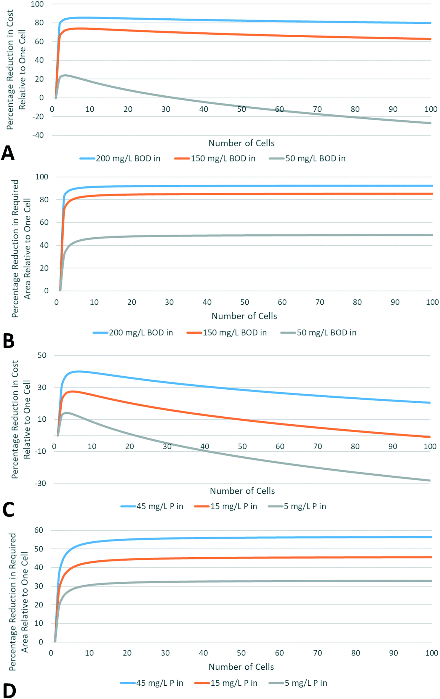Fig. 1 Effect of varying the number of wetland cells on required overall area and treatment costs. All reductions are relative to using one single cell. All biochemical oxygen demand (BOD) plots are for 5000 m³ d⁻¹ influent of varying concentration, with an output concentration of 30 mg L⁻¹. All phosphorus (P) plots are for 5000 m³ d⁻¹ influent of varying concentration, with an output concentration of 1 mg L⁻¹. Plots are A: reduction in total cost for BOD removal, B: reduction in required area for BOD removal, C: reduction in total cost for phosphorus removal, D: reduction in required area for phosphorus removal.

Possible area savings tend to be significantly larger for BOD removal than P and nitrogen (N) removal, and increase more rapidly with input pollutant concentration. This is due to the much higher background concentrations in BOD removal wetlands, which have also been assumed to increase with input concentration (as detailed in the Methodology section). While such reductions in area with increasing wetland cells may appear surprisingly large, they are in line with trends reported by Kadlec and Wallace, who do not investigate the effect on process economics.³⁴ For all pollutants, area and cost savings relative to one single cell were found to be far more dependent on pollutant input and output concentrations than on flow rate.

Nutrient removal costs. Full contour plots for the costs of nutrient removal with input concentration and flow rate are provided in the ESI.†

Fig. 2 shows the cost of remediation for each nutrient, for a range of input and effluent conditions. For removal of all nutrients (BOD, P, TN), economies of scale are initially significant, with an exponent of around 0.8 and as a result volumetric treatment costs at 10000 m³ d⁻¹ are around half of those at 50m³ d⁻¹. However, as size increases the exponent increases to around 0.9, and volumetric costs tend to plateau, leading to relatively little change above 5000 m³ d⁻¹. In the ranges investigated, the volumetric costs for BOD removal tend to be significantly lower than those for P and N removal, and economies of scale tend to decrease more slowly with flow rate. This is due to higher BOD removal rates, leading to generally lower required areas. When designing for simultaneous removal of multiple contaminants in a wetland system, it is common for one contaminant to act as a “bottleneck” and dictate required size and cost. From this range of results it can be concluded that tertiary treatment (i.e. P and N removal) will tend to significantly increase costs relative to secondary treatment (only BOD removal), particularly P removal. For all contaminants, particularly N and BOD, volumetric costs are more sensitive to changes in effluent concentrations than influent concentrations. This is due to the first-order removal rate model, which leads to lower removal rates approaching the background concentration.

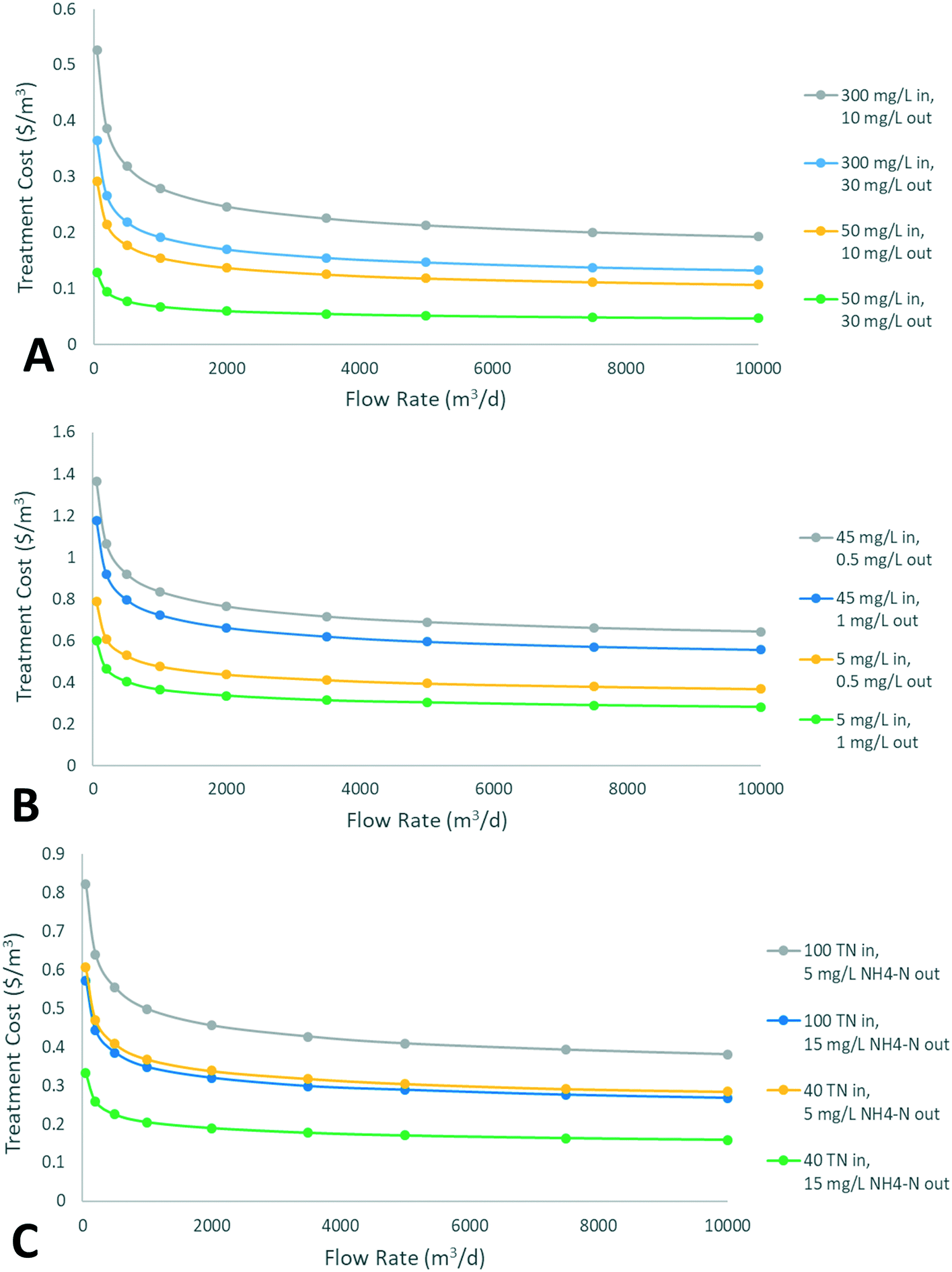Fig. 2 Volumetric costs of nutrient removal using constructed wetlands, for a range of input and output conditions. Plots are A: biochemical oxygen demand (BOD) removal, B: phosphorus (P) removal, C: total nitrogen (TN) removal, assuming input nitrogen made up of 50% organic nitrogen and 50% ammonia nitrogen (NH₄–N).

No general method for estimating the costs of conventional remediation was found, which typically takes place through a form of activated sludge process, possibly followed by further treatment. A direct comparison of costs for wetland remediation and conventional remediation would involve process design considerations for each input condition due to the case-specific nature of wastewater treatment, beyond the scope of this study. Calculated costs of constructed wetland remediation were therefore compared with literature values for conventional secondary and tertiary wastewater treatment,^{22,57,78–87} with results displayed in Fig. 3. All sources were for countries with a similar level of economic development to the U.S.A. All conventional costs were adjusted to 2018 USD by first converting currencies using historical exchange rates, and then applying the CEPCI for the relevant years.

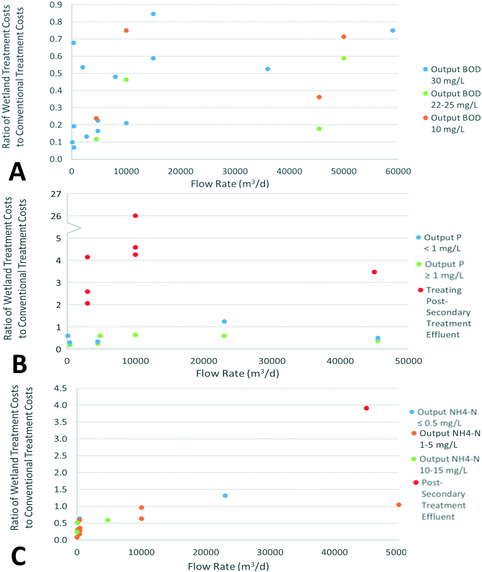Fig. 3 Ratio of simulated wetland remediation costs to reported conventional remediation costs in literature, for BOD, phosphorus, and nitrogen removal. Plots are A: biochemical oxygen demand (BOD) removal, B: phosphorus (P) removal, C: nitrogen removal. NH₄–N corresponds to the concentration of ammonia nitrogen.

By comparing reported costs from various studies with the equivalent costs calculated using this study's methodology, high-level conclusions may be drawn. The following conditions are identified as most economically competitive for constructed wetland remediation:

• Treatment to secondary treatment standards, i.e. BOD removal. Cost estimates for this category of wetland were found to be over 25% cheaper than 86% of reported data. Costs appeared to generally become more similar at higher flow rates, e.g. above 30 000 m³ d⁻¹. This is expected due to economies of scale, although there are few high-flow data points.

• Integrated secondary and tertiary treatment for P and N removal, found to be over 25% cheaper than 91% and 81% of reported data respectively. Removal of P appears to be significantly cheaper than conventional remediation to levels around 0.5 mg L⁻¹, with fairly little data available below this threshold. Removal of N appears economically favourable to outputs around 1 mg L⁻¹ NH₄–N. Wetland costs may be considered to be generally cheaper up to around 10 000 m³ d⁻¹ for removal of both contaminants. Above this threshold limited data was found, but appeared to favour conventional remediation for N removal, and varied for P removal.

• Integrated second and tertiary treatment for small flow rates (below around 500 m³ d⁻¹), even for relatively stringent discharge conditions such as phosphorus and ammonia concentrations below 0.5 mg L⁻¹.

Small flow rates are found to be the condition where constructed wetlands are most economically competitive, as well as least land intensive. The application of wetland wastewater treatment in smaller communities is thus most promising, and there is likely the most available land near such communities. Wetland remediation of wastewater was found to be least economically viable for tertiary treatment of secondary-treated wastewater, with costs significantly higher than conventional alternatives (2–26 times higher). However, this is primarily attributed to the studies considering upgrading existing secondary treatment facilities, thus avoiding significant costs. It may also be attributed to the assumed first-order removal kinetics, leading to low removal rates at low concentrations and thus large area requirements in order to reach strict discharge limits.

The optimum number of cells was investigated for flow rates between 10 and 50 000 m³ d⁻¹. BOD inputs ranged from 50–300 mg L⁻¹, P inputs from 5–45 mg L⁻¹, and total nitrogen from 30–100 mg L⁻¹ (assuming half organic nitrogen and half ammonia nitrogen). Output concentrations were taken as 30 mg L⁻¹ BOD, 1 mg L⁻¹ P, and 5 mg L⁻¹ ammonia nitrogen. The optimum number of cells for BOD removal ranged from 2 to 18 with maximum area of 10 ha, with both the size and number of cells increasing with flow rate and input concentration. Phosphorus and nitrogen removal were found to require a similar number of cells, 2–16 and 1–13 cells respectively. However, cell sizes were much larger, with a maximum size of 55 ha and 54 ha for P and N removal respectively.

Uncertainty. There is a degree of uncertainty with several parameters used in the wetland sizing and costing approach used in this study. Two sets of Monte Carlo simulations were carried out to investigate the variability of results:

1. The variation of design parameters on output concentrations. Wetlands were sized using the methodology currently outlined for secondary and tertiary treatment of municipal wastewater. Contaminant removal rates were then varied based upon the frequency distribution given in the work of Kadlec and Wallace.³⁴ Additionally, precipitation and evapotranspiration factors were varied randomly between 0–2 cm d⁻¹ and 0–1 cm d⁻¹ respectively. All output concentrations were multiplied by the 90% exceedance multiplier to give the target output concentration rather than the design output concentration. As sizing parameters were varied, a range of output effluent concentrations was obtained. The proportion of this range below the target concentration was determined. Correlation coefficients were also calculated, using all output values and the corresponding varied input factors. Results are displayed in Fig. 4.

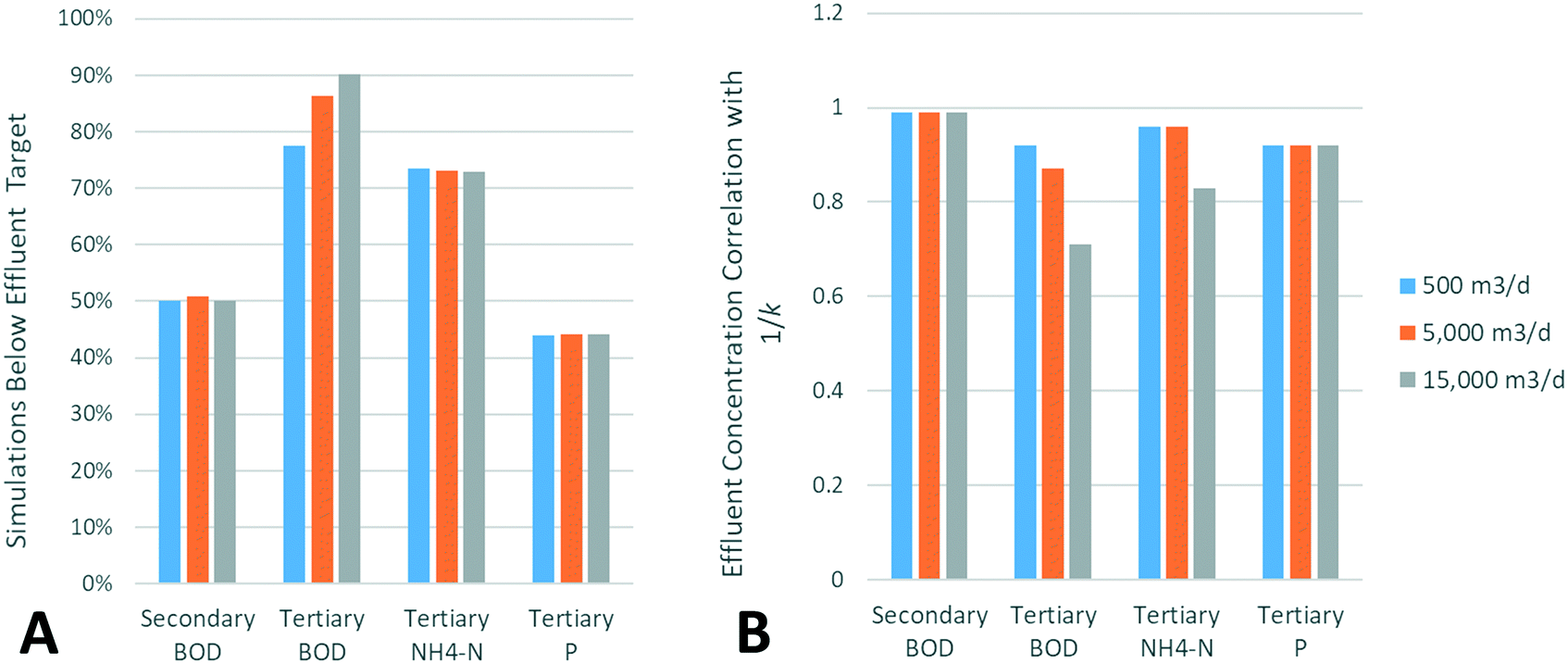Fig. 4 Effect of varying design parameters on simulated effluent concentrations in a Monte Carlo simulation, for secondary treatment and tertiary treatment. Plots are A: proportion of simulations achieving output concentrations below targets concentrations; B: correlation of effluent output concentrations with removal rate constant. BOD refers to biochemical oxygen demand, P refers to phosphorus, NH₄–N refers to ammonia nitrogen, and k corresponds to the first-order removal rate constant of each contaminant. Values in plot A refer to a proportion of the full range of simulated results, coefficients in plot B were calculated using all simulated inputs and outputs; there are therefore no error bars.

2. The effect of economic parameter variation on overall cost, for secondary and tertiary treatment of domestic wastewater. Land costs were varied between 0 and 200 000 $ per ha, construction costs were varied between 50% and 150% of the cost function used, operating costs were varied between $2000 per ha y⁻¹ and $12 000 per ha y⁻¹, and indirect costs were varied between 0% and 100% of total capital costs. The parameters varied in the first Monte Carlo simulation were kept constant. The range of calculated costs are displayed in Fig. 5, as a mean with error bars representing standard deviation.

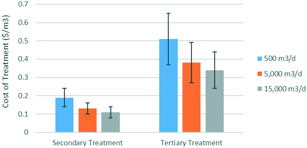Fig. 5 Effect of varying economic parameters on simulated wetland treatment costs in a Monte Carlo simulation, for secondary treatment and tertiary treatment. Error bars represent one standard deviation in the range of simulated results.

Simulation 1 consistently shows that for secondary treatment, around 50% of simulations give output effluents below the design target. When investigating the parameters used in each run, there is a clear correlation between the output concentration and 1/k, with this effect far exceeding that of precipitation and evapotranspiration. Median k-values, as reported by Kadlec and Wallace,³⁴ were used in this study, explaining the proportion of simulations reaching the effluent target being around 50%. For tertiary treatment, phosphorus removal is the limiting factor in wetland sizing, thus displaying the lowest proportion of simulations with output concentrations below the discharge limit, around 45%. As a result, there is therefore a strong correlation with the 1/k value. Determination of the k-factor for the limiting contaminant(s) at a specific site can therefore be identified as the most important aim for real-life wetland design. For BOD and N removal, the wetland is larger than required to reach discharge limits, leading to a much higher proportion of simulations achieving the effluent target. In addition, as concentrations thus approach background concentrations, they exhibit decreasing removal due to the first-order removal rates, and the correlation with 1/k decreases significantly. The proportion of simulations achieving target BOD effluents increases with flow rate, likely due to the higher number of cells used, with decreasing BOD background concentrations in each cell.

Simulation 2 demonstrates that costs are moderately sensitive to the assumed cost parameters, with the standard deviation of overall cost equal to between one third and one quarter of the mean value. However, considering the large cost ranges investigated, these standard deviations are small enough to maintain the high-level conclusions drawn from comparison with literature. Investigation of correlations are shown in Fig. 6. For smaller areas, construction costs appear to have the highest influence on overall costs. However, as the required wetland size increases, operation and maintenance (O&M) costs eventually dominate as economies of scale reduce the relative impact of construction costs and indirect costs. The impact of varying land costs from 0 to $200 000 per ha is seen to have a very weak correlation to overall remediation costs, offering flexibility in terms of location.

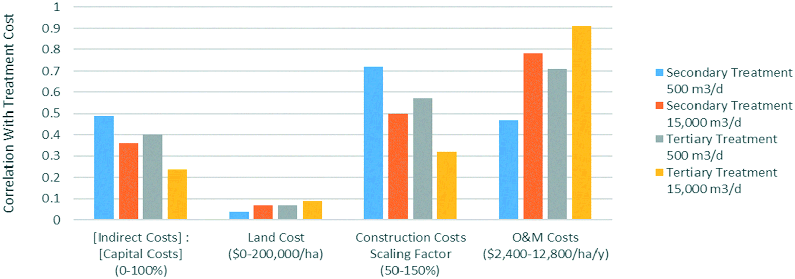Fig. 6 Correlation between varied economic parameters and simulated wetland treatment costs in a Monte Carlo simulation, for secondary treatment and tertiary treatment of domestic wastewater. Correlation coefficients were calculated using the full range of simulated results, and there are therefore no error bars.

Acid mine drainage remediation

Low-pH Drainage. The costs of anaerobic HSSF and VF wetland remediation relative to chemical remediation were calculated for low-pH AMD, using input acidity concentration and flow rate as independent variables, for both maximum and minimum acidity removal rate. Results are displayed in Fig. 7. In addition, nine different AMD scenarios were simulated to compare the costs of wetland remediation and chemical neutralisation, based on the conditions simulated by Skousen when comparing the costs of different chemical remediation schemes.⁸⁸ Their details are shown in Table 2, and are plotted in Fig. 7. In the following analysis, economically favourable conditions are considered to be those where wetland remediation is found to be over 25% cheaper than conventional remediation and economically competitive where wetland remediation is found to be within 25% of the costs of conventional remediation.

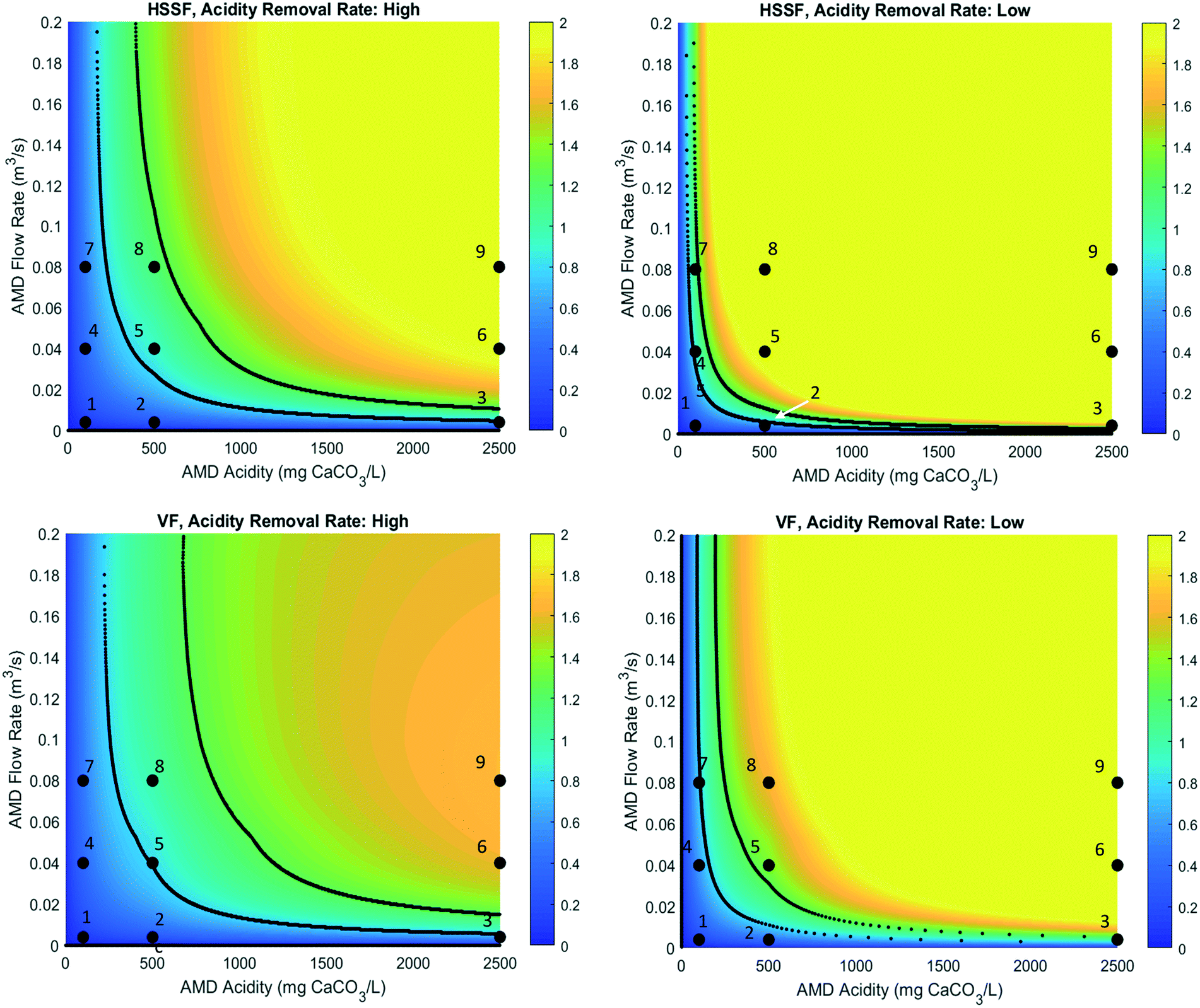Fig. 7 Ratio of wetland remediation costs to conventional remediation costs of low-pH AMD, for HSSF and VF designs with high and low acidity removal rates. The 9 numbered points plotted are scenarios 1–9, as described in Table 2. The area to the left of the black lines represents the economically favourable zone, the middle area between the lines represents the economically competitive zone, and the area to the right of the black lines represents the economically unfavourable zone.

Table 2 Simulated low-pH AMD scenarios. Cells highlighted in green represent cases where wetland remediation is economically favourable, orange for economically competitive, and red for economically unfavourable. High rate and low rate refer to the assumed acidity removal rate

---

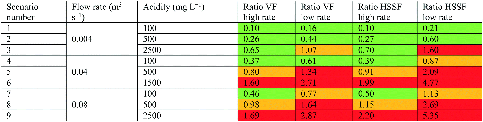
Fig. 7 shows there is a range of conditions under which wetland remediation of AMD appears to be economically competitive or favourable relative to chemical remediation. This is particularly true at low flow rates and/or acidities, where the capital costs of building a chemical plant become prohibitive. However, this may also be partly due to the zero-order removal rate assumption, which may become less accurate at low acidity inputs. For cases with flow rates under around 0.02 m³ s⁻¹ and acidities under around 300 mg L⁻¹, wetland remediation is economically competitive regardless of acidity removal rate. However, results tend to be very sensitive to the assumed acidity removal rate, which varies significantly in literature. When a high acidity removal rate is assumed, wetland remediation is found to be economically competitive for a range of input acidities up to around 500 mg L⁻¹ above 0.04 m³ s⁻¹. However, in the case of a low removal rate, only acidities up to around 180 mg L⁻¹ are competitive for such flows. Additionally, as acidities increase to high levels (above around 1500 mg L⁻¹), the cost effectiveness of wetland remediation is very sensitive to the flow rate. As such, careful design and preparatory studies would be required for wetland remediation at these conditions.

As the economically favourable conditions are at low flows and/or acidities, the associated areas tend to be of moderate size. For HSSF designs, the required areas in these regions are under 26 ha and 22 ha for high and low acidity removal rates respectively. For VF designs, the required areas are under 9 ha for both assumed removal rates. As wetland remediation of AMD has yet to be implemented on a very large scale, the low areas required at the most economically viable conditions may encourage implementation of this technology. Should the technology thus establish itself, a subsequent decrease in capital costs may increase the range of economically viable conditions to eventually include large wetlands handling large and/or highly acidic flows.

The least economically viable are those with high flows and acidity: flows with acidity above 1000 mg L⁻¹ and flows above 0.06 m³ s⁻¹ are economically unviable in all scenarios. However, in the range of representative scenarios, the majority are not within this region, and are either within or closer to the economically viable zone:

• Scenarios 1 and 2 are always economically favourable, regardless of acidity removal rate or wetland design. These are the scenarios with the lowest flow rates and acidities under 500 mg L⁻¹.

• Scenario 3 is economically favourable for HSSF and VF designs with high removal rates, economically competitive for a low-rate VF design, and economically unfavourable for low-rate HSSF designs. This demonstrates that acidity can still be a determining factor in technology selection at low flow rates.

• Scenario 4 is economically favourable under all conditions except for an HSSF design with a low removal rate, for which it is still economically competitive.

• Scenario 7 is economically favourable under high removal rate and competitive for low removal rates.

• Scenarios 5 and 8 are economically competitive for high-rate designs, and economically unfavourable for low-rate designs.

• Only scenarios 6 and 9 are clearly economically unviable under all configurations.

Costs for VF and HSSF designs were compared for their maximum and minimum acidity removal rates, and mid-range rates. At minimum removal rates, HSSF designs were found to be around 17–48% more expensive for economically favourable and competitive cases. At maximum removal rates for economically competitive and favourable conditions, HSSF designs range from 10% cheaper at the lowest flow rates and acidities, to 22% more expensive than VF designs. Lastly, costs were compared for an HSSF design operating at maximum removal rate, and a VF design at mid-range removal rate. Under these assumptions, VF designs were found to be 2–35% more expensive, with this figure decreasing with acidity and flow rate. Due to the significant effect of varying the removal rate within the reported ranges, it would appear that neither design offers a clear advantage in terms of costs. The main advantage of a VF design over an HSSF design is thus the lower area requirement for a generally similar cost.

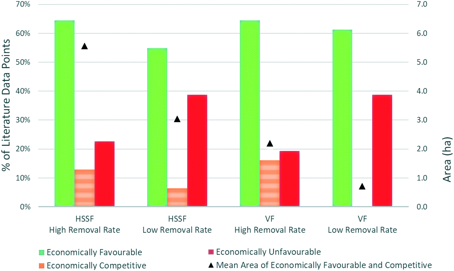
Overall-site low-pH AMD data was sourced from literature, in order to estimate the economic favourability and required size of remediation wetlands for reported AMD cases. Influent metal concentrations, pH, and flow rate were all required for wetland sizing. The former two parameters were relatively well-reported, but flow rates were less common. Furthermore, many of the studies reporting flow rates were for individual output streams at a given site, and not for overall sites. As a result, data was sourced from a relatively small number of studies,^89–92 with the vast majority of figures sourced from two studies: one on Pennsylvanian coal mines, and the other on mines in the Iberian Pyrite Belt.^93,94 Results are presented in Fig. 8.

Fig. 8 Simulated wetland performance for overall-site low-pH AMD, for case study data found in literature.

For all wetland designs and removal rates, over half (55–65%) of the simulated conditions were found to be economically favourable for wetland remediation, 0–16% were found to be economically competitive, and 19–9% were found to be economically unfavourable. When looking at the economically favourable and competitive conditions, the mean wetland area for HSSF designs is 3.05–5.57 ha for low and high removal rates respectively, with the corresponding ranges for VF wetlands being 0.71–2.20 ha. Wetlands with high removal rates have higher mean areas due to the higher areas required for more severe inputs, under which the low removal rate designs are not economically competitive. Thus, under this set of literature data, wetland remediation would appear to be able to play a significant role in remediation of AMD, without requiring impractically large areas. However, although 26 of the 31 data points had acidities within the range of the examples provided by Skousen,⁸⁸ only 8 had flow rates within that range (with most being below 0.004 m³ s⁻¹), and only 7 had both acidity and flow rates within the range of example conditions. This may be interpreted as either the sample size or the example conditions not being widely representative.

Circumneutral-pH drainage. Similarly, the costs of aerobic FWS wetland remediation relative to chemical remediation were calculated for circumneutral AMD, using input Fe concentration and flow rate as independent variables, for both maximum and minimum acidity removal rate. Results are displayed in Fig. 9. Overall trends are similar to those of low-pH AMD remediation: the most economically favourable conditions are those of low flow rate and/or input Fe. However, in this case all generated conditions were found to be economically favourable, for both high and low Fe removal rates and for higher flow rates. It should be noted that even for large required wetland areas (e.g. over 100 ha), costs are still significantly lower than those for conventional treatment, suggesting that practicality issues are likely to constrain wetland remediation of large flows and metal inputs rather than economic ones.

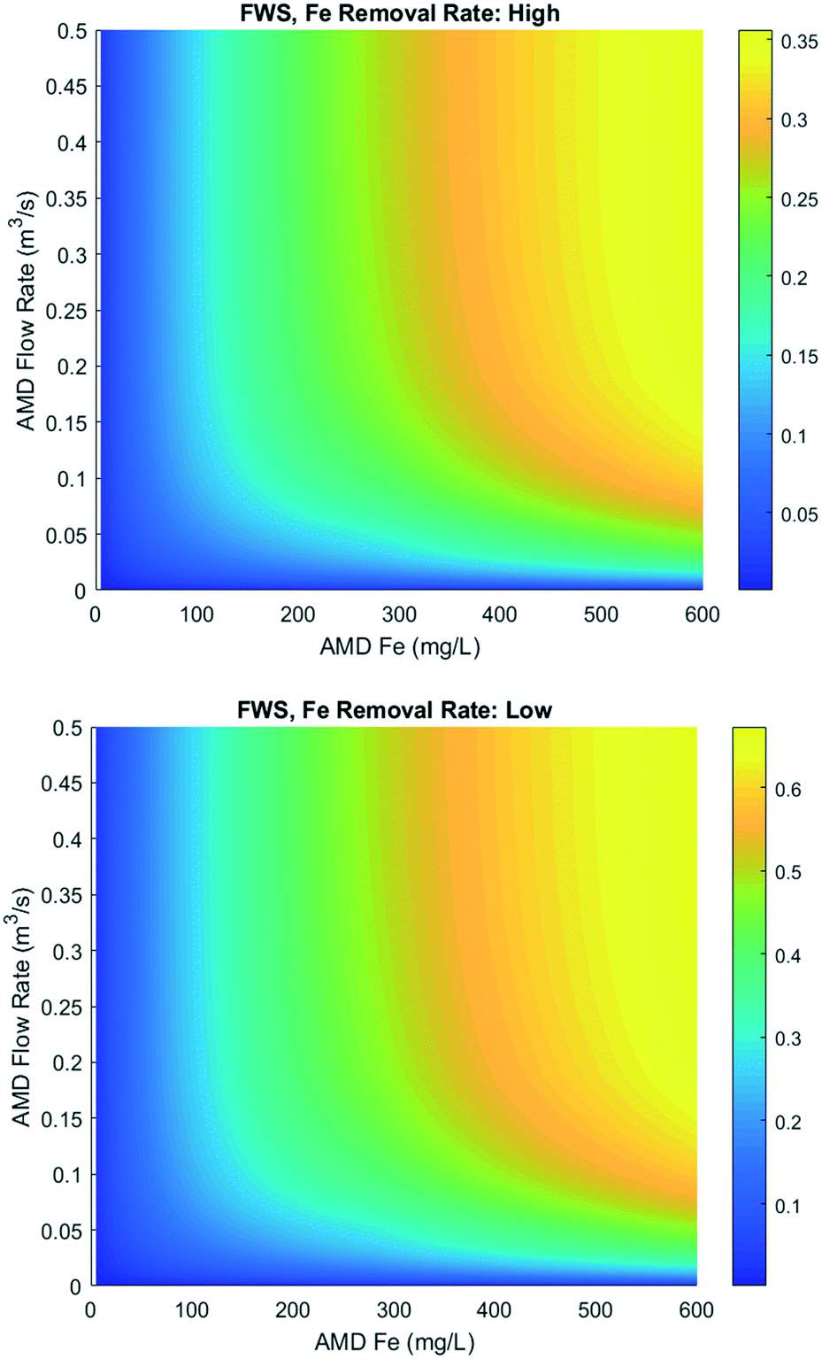Fig. 9 Ratio of wetland remediation costs to conventional remediation costs of circumneutral AMD, for FWS designs with high and low acidity removal rates.

Biomass valorisation

The economic impact of constructed wetland biomass was also investigated as part of this study. This was done by determining the required profit per tonne of biomass generated, under the previously stated assumption of 20 tonnes per ha y⁻¹. Wetlands treating low-pH and circumneutral AMD were investigated, as well as wetlands treating municipal wastewater to secondary and tertiary levels. This analysis was carried out for wetlands greater than 0.5 ha in size, as the required profit quickly escalates to infeasible quantities at low areas. Results are presented in Fig. 10, and are directly proportional to the assumed biomass yield per area.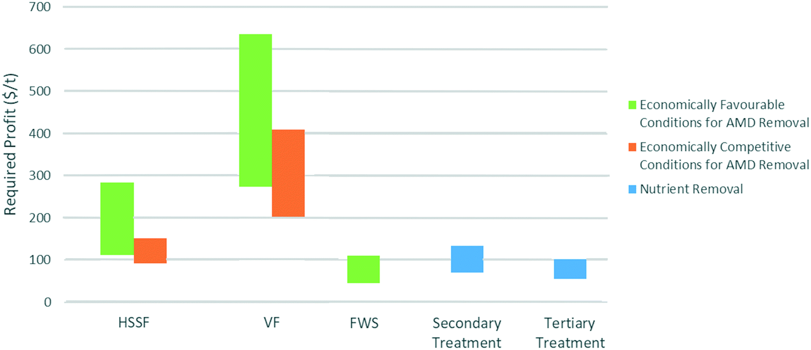

Fig. 10 Required profit per unit dry mass of harvested wetland biomass, in order to offset 10% of total treatment costs. HSSF and VF represent treatment of low-pH AMD using an HSSF and VF wetland design respectively. FWS represents treatment of circumneutral-pH AMD using a FWS wetland design. Secondary treatment and tertiary treatment represent treatment of domestic wastewater using a FWS wetland design.

There is significant variation between required profits depending on the wastewater type, for a 10% reduction in overall costs. Wetlands treating circumneutral-pH AMD and municipal wastewater require profits of the order of $50–100 per tonne of dry biomass. HSSF wetlands treating low-pH AMD require around $110–280 per tonne, while VF wetlands treating low-pH AMD require around $270–630 per tonne. The significantly lower costs for a given flow rate explain the lower required profits for FWS wetlands treating circumneutral-pH AMD and municipal wastewater. For wetlands treating low-pH AMD, VF wetlands require a lower area, which may explain the significantly higher required profits relative to HSSF designs. The similarity between low-removal-rate and high-removal-rate wetlands can be explained: those with low removal rates have higher costs to offset, but this is counterbalanced by the larger areas from which to harvest. However, for all wastewater types, the lowest required profits were for the largest wetlands, which may already be considered to have technical limitations due to their size.

Four possible revenue sources have been considered for comparative purposes: directly selling reeds ($70 per t),^95,96 biorefinery for bioethanol production ($420–1000 per t),^96,97 biorefinery for cellulose pulp production ($450–900 per t),^96,98 and production of reed pellets for fuel use ($140 per t).^95,99 All revenue options are heavily dependent on the achievable profit margin, which will vary with the scale of operation. As a result, thorough analysis into the process economics of each route and market size is required, which has been considered beyond the scope of this study. However, some preliminary analysis on the feasibility of several options has been carried out by Croon in a 2014 study, which considers the utilisation of reed biomass purchased at $70 per t.⁹⁶ While technologically feasible, the major obstacles to reed utilisation are identified as the costs of harvest and transport to processing plants, and the large scales needed for economical production. Integration of wetland remediation with reed processing may allow harvest and transport costs to be essentially absorbed into wetland O&M costs: Croon's study concerns harvesting of natural reed beds which have no such costs. Furthermore, harvest and transport costs are reported to be in the range of $600 per ha, corresponding to 9% of the O&M costs assumed in this study, and significantly smaller than the uncertainty in O&M costs based on review of literature.¹⁰⁰

The major practical drawback would thus appear to be required areas for minimum economic production. Croon gives minimum economic productions of 50 000 t y⁻¹, 150 000 t y⁻¹, and 60 000 t y⁻¹ for bioethanol, pulp, and pellets respectively. However, in 2016 26.2% of pulp mills in Europe operated at under 100 000 t y⁻¹, and 5.9% under 25 t y⁻¹, with this latter figure instead being used as the minimum economic production.¹⁰¹ The required areas for bioethanol, pulp, and pellet production are thus calculated to be 19 400 ha, 3600 ha, and 3000 ha. It should be noted that these figures assume 35% cellulose content, no cellulose degradation, 80% sugar release yield, and 90% ethanol yield, and are therefore different to those calculated by Croon. Required areas are clearly substantial, and would need to be distributed among a number of large wetland sites, which tend to be least economically favourable. Therefore, this is only likely to be feasible if wetland remediation were to become more established.

In the case of bioethanol production, it may be possible to blend wetland biomass with different feedstocks in a general pretreatment process. In the NREL's technoeconomic analysis of a lignocellulosic bioethanol plant producing 218 000 t y⁻¹ of bioethanol from corn stover, feedstock costs (including handling) were found to account for 34% of total bioethanol production costs.¹⁰² Therefore, the blending of wetland biomass could still allow substantial cost reductions while reducing the required wetland area. Additionally, the magnitude of possible savings could reduce the required minimum economic production capacity of smaller bioethanol plants using only wetland biomass, thus reducing area requirements.

Anaerobic digestion (AD) to produce biogas may represent a more appropriate option for smaller-scale, more disaggregated implementation of constructed wetlands. Development of small-scale anaerobic digesters for localised biogas production has been considered a promising route for energy and fertiliser provision in small communities in developing countries.^103,104 In addition to wetland biomass, a range of feedstocks can be used in AD such as other types of biomass or animal waste.¹⁰⁵ Small-scale AD may thus allow the combination of wetland remediation of agricultural and domestic wastewater with localised energy production. Although digestion on a small scale for local use may not significantly affect overall economics of wetland remediation, its advantages could prove particularly attractive to small communities in developing countries, and thus help instigate more widespread adoption of CWs.

The effect of possible metal recovery was also investigated for wetlands treating AMD, possible for instance through ionic liquid pretreatment of metal-contaminated feedstocks.¹⁰⁶ The theoretical maximum metal recovery was found to be extremely low, even with the optimistic assumed biomass metal uptake: around 2 kg ha⁻¹ y⁻¹ of Fe and Al, 1 kg ha⁻¹ y⁻¹ of Mn and 100 g ha⁻¹ y⁻¹ of trace metals, providing negligible economic impact. Uncertainty in the values for biomass growth rate and metal uptake are very unlikely to affect this conclusion. The reason for such low uptake is that the main metal removal mechanisms in wetlands involve immobilisation in the sediment. Additionally, the wetland species typically used are metal-tolerant or moderately metal-accumulating rather than hyper-accumulating. While hyper-accumulating species may allow more significant metal recovery, growth rates of such species tend to be low, and their accumulating capacities tend to only apply to a small number of metals per species. However, despite the lack of economic benefit, the possibility of utilising metal-contaminated wetland biomass would solve the disposal issue from AMD wetlands.^107,108 Additionally, should metal concentrations in wetland sediment reach high levels that require end-of-life disposal, the feasibility of treating the generated metal-concentrated sludge for metal recovery may be investigated.

Conclusions

This study has demonstrated that constructed wetlands offer an economically viable method for remediation of wastewater under a wide range of conditions, for both nutrient removal and remediation of low-pH and circumneutral acid mine drainage. The P-k-C* model was used to size FWS wetlands for removal of BOD, phosphorus, and nitrogen, which incorporates a first-order areal removal model with a background concentration. A wide range of input contaminant concentrations and flow rates were simulated, and the costs calculated for remediation to various effluent standards. These costs were found by using a construction cost function from literature, to which provisions for land costs and indirect costs were explicitly added, and mid-range O&M costs based on examination of literature.

Wetlands used for nutrient removal were found to have an optimum number of cells, at which decreased area requirements from improved hydraulic performance counterbalance the increased cost of each smaller cell. By optimising cell number, economic savings of up to 86% and 42% were found for BOD and P removal over the ranges investigated. When compared to literature values, wetland remediation was found to be most suitable for secondary treatment of municipal wastewater, both at low and high flow rates. When considering tertiary treatment of wastewater, wetland remediation was found to be economically competitive for integrated secondary and tertiary to stringent standards (around 0.5 mg L⁻¹ phosphorus and 1 mg L⁻¹ ammonia nitrogen), also particularly at low flow rates but remaining competitive above 10 000 m³ d⁻¹. For tertiary treatment of post-secondary treatment wastewater, wetland remediation were significantly more expensive than conventional treatment methods. The uncertainty of the sizing and costing estimates were investigated using two separate Monte Carlo simulations. The first found a strong correlation (r > 0.9, p < 0.01) between the wetland size and the reciprocal of the contaminant removal rate, for the “bottleneck” contaminant, with no significant correlation for precipitation and evapotranspiration rates. The second found costs to be most sensitive to variations in capital costs for small wetlands, and to O&M costs with increasing size. Land costs were found to have little impact on overall costs.

Wetland remediation of circumneutral AMD was found to be economically favourable relative to chemical dosing under all conditions investigated, and particularly at low flow rates and Fe concentrations. For low-pH AMD, wetland remediation was found to be economically competitive at a fairly limited range of flow rates and acidities, with this range particularly sensitive to the assumed acidity removal rate. However, a significant proportion of simulated realistic AMD conditions were found to fall within the economically favourable and competitive zones, as well as a majority of overall-site literature data. No clear economic advantage which could be ascertained between VF and HSSF designs due to the large ranges of removal rates from literature. However, the VF design tended to require a lower area requirement for similar costs.

The possibility of utilising the wetland biomass to offset costs was explored, for direct biomass sale, production of pellets, digestion to biogas, and biorefinery to bioethanol, and pulp. While it was not possible to quantitatively determine the most suitable product, practicality barriers were identified, particularly regarding the required wetland area. A biorefinery with metal recovery was found to have a negligible economic impact but did, however, present a method to utilise contaminated biomass which may otherwise be regarded as a waste product of wetland AMD remediation.

There remains several areas for future work with regards to high-level modelling of wetland remediation. The first, as highlighted by the Monte Carlo analysis, is increased removal rate data, with an aim to reduce the uncertainty introduced by the wide range of removal rate estimates or to gain a better understanding of high-level parameters affecting the removal rate. Additionally, there remains scope for development of high-level wetland remediation models. The P-k-C* model has been shown to be the most suitable for SSF wetlands in a review by Rousseau et al., and represents an improvement upon the first-order k-C* model.¹⁰⁹ However, several of the limitations of the first-order k-C* model outlined by Kadlec may still be improved upon.¹¹⁰ Multiple studies have tested a first-order removal rate model for certain metals, but the use of such a model for general wetland design would require additional studies with well-reported design properties in order to more confidently estimate the relevant removal rates, background concentrations and P_TIS values.^27,111,112 While sophisticated packages do exist for constructed wetland performance, they are intended for detailed design of individual wetlands, and may thus be considered too detailed for this type of high-level estimate. Such models are included in Meyer et al.'s review into the modelling of constructed wetlands, who also emphasise the need for increased data collection and availability.¹¹³

Conflicts of interest

There are no conflicts to declare.

Acknowledgements

The authors would like to thank the Engineering and Physical Sciences Research Council (EPSRC) for a Doctoral Training Programme studentship for AF and additional funding through the Supergen Bioenergy Hub (EP/S000771/1).

Notes and references

1. U. Nations, Three pillars of UNESCO activities on water, 2015, http://unesdoc.unesco.org/images/0024/002436/243651e.pdf.
2. R. Johnston, Arsenic and the 2030 Agenda for Sustainable Development, 2016, pp. 12–14,  DOI:10.1201/b20466-7.
3. E. Corcoran, C. Nellemann, E. Baker, R. Bos, D. Osborn and H. Savelli, Sick Water? The Central Role of Wastewater Management in Sustainable Development. A Rapid Response Assessment, United Nations Environment Programme, UN-HABITAT, GRID-Arendal, 2010,  DOI:10.1007/s10230-011-0140-x.
4. M. Goutard and UNESCO Project, Int. J. Early Child., 1990, 22(2), 1–4.
5. FAO and IWMI, More People, More Food, Worse Water? A Global Review of Water Pollution from Agriculture, 2018, http://www.fao.org/policy-support/resources/resources-details/en/c/1144303/%0Ahttp://www.fao.org/3/ca0146en/CA0146EN.pdf.
6. R. P. Schwarzenbach, T. Egli, T. B. Hofstetter, U. von Gunten and B. Wehrli, Global Water Pollution and Human Health, Annu. Rev. Environ. Resour., 2010, 35(1), 109–136,  DOI:10.1146/annurev-environ-100809-125342.
7. Reducing Inequalities in Water Supply, Sanitation, and Hygiene in the Era of the Sustainable Development Goals, Reducing Inequalities Water Supply, Sanit Hyg Era Sustain Dev Goals, 2017,  DOI:10.1596/27831.
8. OECD (Organisation for Economic Co-operation and Development), Environmental Outlook to 2050: Key Findings on Water, 2012;(March).
9. UNDP, WWDR 2015: Water for a Sustainable World, 2015,  DOI:10.1016/S1366-7017(02)00004-1.
10. T. A. Larsen, M. Maurer, K. M. Udert and J. Lienert, Nutrient cycles and resource management: Implications for the choice of wastewater treatment technology, Water Sci. Technol., 2007, 56(5), 229–237,  DOI:10.2166/wst.2007.576.
11. V. H. Smith, Eutrophication of Freshwater and Coastal Marine Ecosystems - A Global Problem, Environ. Sci. Pollut. Res., 2003, 10(2), 126–139,  DOI:10.17660/ActaHortic.2017.1170.71.
12. M. F. Chislock, E. Doster, R. A. Zitomer and A. E. Wilson, Eutrophication: Causes, Consequences, and Controls in Aquatic Ecosystems, Nature Education Knowledge, 2013, 4(4), 10.
13. R. Howarth, F. Chan and D. J. Conley, et al. Coupled biogeochemical cycles: Eutrophication and hypoxia in temperate estuaries and coastal marine ecosystems, Front. Ecol. Environ., 2011, 9(1), 18–26,  DOI:10.1890/100008.
14. S. R. Carpenter, N. F. Caraco, D. L. Correll, R. W. Howarth, A. N. Sharpley and V. H. Smith, Nonpoint Pollution of Surface Waters With Phosphorus and Nitrogen, Ecol. Appl., 1998, 8(3), 559–568.
15. W. K. Dodds, W. W. Bouska and J. L. Eitzmann, et al. Policy Analysis Policy Analysis Eutrophication of U. S. Freshwaters: Damages, Environ. Sci. Technol., 2009, 43(1), 12–19,  DOI:10.1021/es801217q.
16. N. N. Rabalais, Nitrogen in Aquatic Ecosystems, Ambio, 2002, 31(2), 102–112,  DOI:10.1579/0044-7447-31.2.102.
17. S. Nixon, Coastal marine eutrophication: A definition, social causes, and future concerns, Ophelia., 1995, 45(1), 199–219.
18. E. M. Bennett, S. R. Carpenter and N. F. Caraco, Human Impact on Erodable Phosphorus and Eutrophication: A Global Perspective, Bioscience., 2006, 51(3), 227,  DOI:10.1641/0006-3568(2001)051[0227:hioepa]2.0.co;2.
19. P. Drechsel, M. Qadir and D. Wichelns, Wastewater: Economic asset in an urbanizing world, Wastewater Econ Asset an Urban World, 2015, pp. 1–282,  DOI:10.1007/978-94-017-9545-6.
20. J. Peirce, R. Weiner and P. Vesilind, Wastewater Treatment, Environ. Pollut. Control J., 1998, 105–123,  DOI:10.1016/B978-0-7506-9899-3.50009-2.
21. M. Samer, Biological and Chemical Wastewater Treatment Processes, vol. i, 2015.
22. F. Jiang, M. Beck, R. Cummings and K. Rowles Estimation of costs of phosphorus removal in wastewater treatment facilities: construction de novo, Water Policy Work Pap #2004-010, 2004,(June), pp. 1–28, http://www2.gsu.edu/~wwwenv/waterPDF/W2004010.pdf.
23. S. Yeoman, T. Stephenson, J. N. Lester and R. Perry, The removal of phosphorus during wastewater treatment: A review, Environ. Pollut., 1988, 49(3), 183–233,  DOI:10.1016/0269-7491(88)90209-6.
24. M. Libhaber, Appropriate Technologies for Wastewater Treatment and Effluent Reuse for Irrigation - http://siteresources.worldbank.org/EXTWAT/Resources/4602122-1213366294492/5106220-1234469721549/27.2_WWT_Carbon_Footprint.pdf.
25. A. S. Sheoran and V. Sheoran, Heavy metal removal mechanism of acid mine drainage in wetlands: A critical review, Miner. Eng., 2006, 19(2), 105–116,  DOI:10.1016/j.mineng.2005.08.006.
26. US Environmental Protection Agency, Acid Mine Drainage Prediction, Acid Mine Drain Predict EPA 530-R-94-036, 1994;(December), p. 52, EPA 530-R-94-036.
27. P. L. Younger, S. Banwart and R. S. Hedin, Mine Water: Hydrology, Pollution, Remediation, 2002.
28. Authority NR, Abandoned Mines A Report of the National Rivers Authority, 1994;(March).
29. EPA, Hardrock Mining Framework - Appendix A, 1997.
30. Mine Environment Neutral Drainage, Report of Results of a Workshop on Mine Reclamation, 1994;(August).
31. D. B. Johnson and K. B. Hallberg, Acid mine drainage remediation options: A review, Sci. Total Environ., 2005, 338(1–2), 3–14,  DOI:10.1016/j.scitotenv.2004.09.002.
32. M. S. Fennessy, W. J. Mitsch, M. S. Fennessy and W. J. Mitsch, Treating coal mine drainage with an artificial wetland, Res. J. Water Pollut. Control Fed., 1989, 61(11), 1691–1701.
33. B. Gazea, K. Adam and A. Kontopoulos, A review of passive systems for the treatment of acid mine drainage, Miner. Eng., 1996, 9(1), 23–42,  DOI:10.1016/0892-6875(95)00129-8.
34. R. H. Kadlec and S. D. Wallace, Treatment wetlands, Treat Wetl. 2009, p. 965, DOI:10.1002/1521-3773(20010316)40:6<9823::AID-ANIE9823>3.3.CO;2-C.
35. J. Vymazal, Constructed Wetlands for Wastewater Treatment, Water., 2010, 25(5), 353–369,  DOI:10.1016/B978-0-08-088504-9.00249-X.
36. H. Wu, J. Zhang and H. H. Ngo, et al. A review on the sustainability of constructed wetlands for wastewater treatment: Design and operation, Bioresour. Technol., 2015, 175, 594–601,  DOI:10.1016/j.biortech.2014.10.068.
37. J. Vymazal, Constructed wetlands for treatment of industrial wastewaters: A review, Ecol. Eng., 2014, 73, 724–751,  DOI:10.1016/j.ecoleng.2014.09.034.
38. J. Vymazal and T. Březinová, The use of constructed wetlands for removal of pesticides from agricultural runoff and drainage: A review, Environ. Int., 2015, 75, 11–20,  DOI:10.1016/j.envint.2014.10.026.
39. J. Vymazal, The use constructed wetlands with horizontal sub-surface flow for various types of wastewater, Ecol. Eng., 2009, 35(1), 1–17,  DOI:10.1016/j.ecoleng.2008.08.016.
40. P. Cooper, The Constructed Wetland Association's Database of Constructed Wetland Systems in the UK, in: Wastewater Treatment, Plant Dynamics and Management in Constructed and Natural Wetlands, 2008.
41. South Florida Water Management District, Stormwater Treatment Area 2 Operation Plan, 2011;(September).
42. L. Osmanaj, A. Haxhikadrija, P.-H. Dodane and A. Vokshi, Potential of Constructed Wetland for Wastewater Treatment in Rural Areas in Kosovo, J. Hydrol. Eng., 2015, 1, 27–34,  DOI:10.17265/2332-8215/2015.01.003.
43. A. S. Juwarkar, B. Oke, A. Juwarkar and S. M. Patnaik, Domestic wastewater treatment through constructed wetland in India, Water Sci. Technol., 1995, 32(3), 291–294.
44. V. M. Lakay, An Analysis of the Performance of Constructed Wetlands in the Treatment of Domestic Wastewater in the Western Cape, South Africa, MSc, University of Cape Town, 2012.
45. O. Alagbe and G. M. Alalade, Implications of Constructed Wetlands Wastewater Treatment for Sustainable Planning in Developing World, 2013.
46. M. L. Solano, P. Soriano and M. P. Ciria, Constructed Wetlands as a Sustainable Solution for Wastewater Treatment in Small Villages, Biosyst. Eng., 2004, 87(1), 109–118,  DOI:10.1016/j.biosystemseng.2003.10.005.
47. A. K. Kivaisi, The potential for constructed wetlands for wastewater treatment and reuse in developing countries: A review, Ecol. Eng., 2001, 16(4), 545–560,  DOI:10.1016/S0925-8574(00)00113-0.
48. P. Denny, Implementation of constructed wetlands in developing countries, Water Sci. Technol., 1997, 35, 27–34,  DOI:10.1016/S0273-1223(97)00049-8.
49. D. Q. Zhang, K. B. S. N. Jinadasa, R. M. Gersberg, Y. Liu, W. J. Ng and S. K. Tan, Application of constructed wetlands for wastewater treatment in developing countries - A review of recent developments (2000-2013), J. Environ. Manage., 2014, 141, 116–131,  DOI:10.1016/j.jenvman.2014.03.015.
50. S. A. W. Diemont, Mosquito larvae density and pollutant removal in tropical wetland treatment systems in Honduras, Environ. Int., 2006, 32(3), 332–341,  DOI:10.1016/j.envint.2005.07.001.
51. T. Zhang, D. Xu, F. He, Y. Zhang and Z. Wu, Application of constructed wetland for water pollution control in China during 1990-2010, Ecol. Eng., 2012, 47, 189–197,  DOI:10.1016/j.ecoleng.2012.06.022.
52. J. L. Faulwetter, V. Gagnon and C. Sundberg, et al. Microbial processes influencing performance of treatment wetlands: A review, Ecol. Eng., 2009, 35(6), 987–1004,  DOI:10.1016/j.ecoleng.2008.12.030.
53. A. M. Nahlik and W. J. Mitsch, Tropical treatment wetlands dominated by free-floating macrophytes for water quality improvement in Costa Rica, Ecol. Eng., 2006, 28(3), 246–257,  DOI:10.1016/j.ecoleng.2006.07.006.
54. B. Gopal, Natural and constructed wetlands for wastewater treatment: Potentials and problems, Water Sci. Technol., 1999, 40, 27–35,  DOI:10.1016/S0273-1223(99)00468-0.
55. D. Liu, Y. Ge and J. Chang, et al. Constructed wetlands in China: Recent developments and future challenges, Front. Ecol. Environ., 2009, 7(5), 261–268,  DOI:10.1890/070110.
56. D. Zhang, R. M. Gersberg and T. S. Keat, Constructed wetlands in China, Ecol. Eng., 2009, 35(10), 1367–1378,  DOI:10.1016/j.ecoleng.2009.07.007.
57. G. McNamara, Economic and Environmental Cost Assessment of Wastewater Treatment Systems A Life Cycle Perspective, PhD, Dublin City University, 2018.
58. L. Cardoch, J. W. Day, J. M. Rybczyk and G. P. Kemp, An economic analysis of using wetlands for treatmnt of shrimp processing wastewater - a case study in Dulac, LA, Ecol. Econ., 2000, 33, 93–101.
59. I. Mannino, D. Franco and E. Piccioni, et al., A Cost-Effectiveness Analysis of Seminatural Wetlands and Activated Sludge Wastewater-Treatment Systems, Environ. Manage., 2008, 41, 118–129,  DOI:10.1007/s00267-007-9001-6.
60. G. R. Watzlaf, K. T. Schroeder, R. L. P. Kleinmann, C. L. Kairies, R. W. Nairn and W. B. Street, The Passive Treatment of Coal Mine Drainage, 2004, pp. 1–72.
61. C. A. Cravotta III and C. S. Kirby, Acidity and Alkalinity in Mine Drainage: Practical Considerations, J. Am. Soc. Min. Reclam., 2004, 2004(1), 334–365,  DOI:10.21000/JASMR04010334.
62. R. Hedin, R. Narin and R. Kleinmann, Passive Treatment of Coal Mine Drainage, 1994.
63. K. L. Ford, Passive Treatment Systems for Acid Mine Drainage, 2003.
64. J. Skousen and P. Ziemkiewicz, Performance of 116 Passive Treatment Systems for Acid Mine Drainage, J Am Soc Min Reclam., 2005, 2005(1), 1100–1133,  DOI:10.21000/JASMR05011100.
65. D. A. Kepler, Wetland Sizing, Design, and Treatment Effectiveness for Coal Mine Drainage, Min Reclam Conf Exhib Charleston, West Virginia April 23-26, 1990.
66. J. Demchak, T. Morrow and J. Skousen, Treatment of acid mine drainage by four vertical flow wetlands in Pennsylvania, Geochem.: Explor., Environ., Anal., 2001, 1(1), 71–80,  DOI:10.1144/geochem.1.1.71.
67. C. Zipper, J. Skousen and C. Jage, Passive Treatment of Acid-Mine Drainage with. Reclam Guidel Surf MINED L. 2011,  DOI:10.2134/jeq1994.00472425002300060030x.
68. H. Brix, R. H. Kadlec, R. L. Knight, J. Vymazal, P. Cooper and R. Haberl, Constructed wetlands for pollution control: process, performance, design and operation, 2000, p. 156, https://es.scribd.com/doc/208541250/Constructed-Wetlands-for-Pollution-Control-Processes-Performance-Design-and-Operation-by-IWA.
69. https://amd.osmre.gov/ .
70. D. B. George, Development of Guidelines and Design Equations for Subsurface Flow Constructed Wetlands Treating Municipal Wastewater, 2000.
71. N. Mburu, Experimental and Modeling Studies of Horizontal Subsurface Flow Constructed Wetlands Treating Domestic Wastewater, 2013, vol. 128,  DOI:10.1017/CBO9781107415324.004.
72. T. Noack and Associates AP, Costs and Other Considerations for Constructed Wetlands Major Cost Categories & Drivers Costs for Example Projects Green Infrastructure Case Study “ Ownership ” of the Project, 2018.
73. J. Vymazal and L. Kropfelova, Wastewater Treatment in Constructed Wetlands with Horizontal Sub-Surface Flow, 2008.
74. Agency USE protection, Wastewater Technology Fact Sheet Wetlands: Subsurface Flow, Environ Prot Agency, 2000, pp. 1–7, EPA 832-F-99-062.
75. United States Environmental Protection Agency, Wastewater Technology Fact Sheet Wetlands: Free Water Surface, Environ Prot Agency, 2000, pp. 1–8, EPA 832-F-00-024.
76. US Department of Agriculture National Agricultural Statistics Service, Land Values 2017 Summary, 2017, (August), pp. 1–22, http://usda.mannlib.cornell.edu/usda/current/AgriLandVa/AgriLandVa-08-03-2017.pdf.
77. Mine Environment Neutral Drainage Program and Canadian Centre for Mineral and Energy Technology, ACID MINE DRAINAGE - STATUS OF CHEMICAL TREATMENT AND SLUDGE MANAGEMENT PRACTICES, 1994.
78. R. Bashar, K. Gungor, K. G. Karthikeyan and P. Barak, Cost effectiveness of phosphorus removal processes in municipal wastewater treatment, Chemosphere, 2018, 197, 280–290,  DOI:10.1016/j.chemosphere.2017.12.169.
79. US EPA, Biological Nutrient Removal Processes and Costs, 2007.
80. B. Papadopoulos, K. P. Tsagarakis and A. YannopoulosCost and Land Functions for Wastewater Treatment Projects : Typical Simple Cost and Land Functions for Wastewater Treatment Projects : Typical Simple Linear Regression versus, 2007, 9372(Setember 2017), pp. p1–7,  DOI:10.1061/(ASCE)0733-9372(2007)133.
81. S. Jafarinejad, Cost estimation and economical evaluation of three configurations of activated sludge process for a wastewater treatment plant (WWTP) using simulation, Appl. Water Sci., 2017, 7(5), 2513–2521,  DOI:10.1007/s13201-016-0446-8.
82. E. Friedler and E. Pisanty, Effects of design flow and treatment level on construction and operation costs of municipal wastewater treatment plants and their implications on policy making, Water Res., 2006, 40(20), 3751–3758,  DOI:10.1016/j.watres.2006.08.015.
83. T. Dogot, Y. Xanthoulis, N. Fonder and D. Xanthoulis, Estimating the costs of collective treatment of wastewater: The case of Walloon Region (Belgium), Water Sci. Technol., 2010, 62(3), 640–648,  DOI:10.2166/wst.2010.322.
84. R. Nogueira, A. G. Brito and A. P. Machado, et al., Economic and environmental assessment of small and decentralized wastewater treatment systems, Desalin Water Treat., 2009, 4(1-3), 16–21,  DOI:10.5004/dwt.2009.349.
85. M. Molinos-Senante, F. Hernández-Sancho, M. Mocholí-Arce and R. Sala-Garrido, Economic and environmental performance of wastewater treatment plants: Potential reductions in greenhouse gases emissions, Resour. Energy Econ., 2014, 38, 125–140,  DOI:10.1016/j.reseneeco.2014.07.001.
86. Inc B& M, Ultra-Low Phosphorus Removal Pilot Study City of Mankato, Minnesota, 2016.
87. US Environmental Protection Agency, Economic Analysis of Final Water Quality Standards for Nutrients for Lakes and Flowing Waters in Florida, 2010, (November).
88. J. Skousen, Overview of Acid Mine Drainage Treatment with Chemicals, Acid Mine Drainage, Rock Drainage, Acid Sulfate Soils Causes, Assessment, Predict Prev Remediat, 2014, 9780470487, pp. 325–337,  DOI:10.1002/9781118749197.ch29.
89. H. Davies, P. Weber, P. Lindsay, D. Craw and J. Pope, Characterisation of acid mine drainage in a high rainfall mountain environment, New Zealand, Sci. Total Environ., 2011, 409(15), 2971–2980,  DOI:10.1016/j.scitotenv.2011.04.034.
90. N. F. Gray, Acid mine drainage composition and the implications for its impact on lotic systems, Water Res., 1998, 32(7), 2122–2134,  DOI:10.1016/S0043-1354(97)00449-1.
91. M. Olías, J. M. Nieto, A. M. Sarmiento, J. C. Cerón and C. R. Cánovas, Seasonal water quality variations in a river affected by acid mine drainage: The Odiel River (South West Spain), Sci. Total Environ., 2004, 333(1-3), 267–281,  DOI:10.1016/j.scitotenv.2004.05.012.
92. C. A. Johnson and I. Thornton, Hydrological and chemical factors controlling the concentrations of Fe, Cu, Zn and As in a river system contaminated by acid mine drainage, Water Res., 1987, 21(3), 359–365,  DOI:10.1016/0043-1354(87)90216-8.
93. J. S. España, E. L. Pamo, E. Santofimia, O. Aduvire, J. Reyes and D. Barettino, Acid mine drainage in the Iberian Pyrite Belt (Odiel river watershed, Huelva, SW Spain), Geochemistry, mineralogy and environmental implications, Appl. Geochem., 2005, 20(7), 1320–1356,  DOI:10.1016/j.apgeochem.2005.01.011.
94. Pensylvania Department of Environmental Protection, Coal Mine Drainage Prediction and Pollution Prevention in Pennsylvania, 1998.
95. P. Icka, R. Damo and E. Icka, Reed Biomass, a Possibility of Cultivation and Protection of “Wetland” in Korça Field in Albania, Annals “Valahia” University of Targoviste – Agriculture, 2017, 11(1), 1–5,  DOI:10.1515/agr-2017-0001.
96. F. W. Croon, Saving reed lands by giving economic value to reed, Mires Peat., 2014, 13, 1–13.
97. https://markets.ft.com/data/commodities/tearsheet/summary?c=Ethanol .
98. https://www.indexmundi.com/commodities/?commodity=wood-pulp&months=360 .
99. D. McNeil and M. RaymentInnovation for reed bed biomass fuel and biodiversity by FIELDFARE – ANALYSIS OF THE OPPORTUNITY, 2015;(Setember), pp. 1–10.
100. UK Department for Energy and Climate Change, Wetland Biomass to Bioenergy Gasification and anaerobic digestion of sustainably - sourced wetland biomass Phase 1 report, 2013;(March).
101. Confederation of European Paper Industries (CEPI), CEPI Key Statistics 2016, CEPI Total Pulp Prod by Ctry 2016, 2017, p. 8https://goo.gl/aFb65d.
102. D. Humbird, R. Davis and L. Tao, et al.Process Design and Economics for Biochemical Conversion of Lignocellulosic Biomass to Ethanol: Dilute-Acid Pretreatment and Enzymatic Hydrolysis of Corn Stover, 2002, http://www.osti.gov/bridge. Accessed May 31, 2020.
103. J. U. Smith, K. Yongabi and H. Black, et al.The Potential of Small-Scale Biogas Digesters to Alleviate Poverty and Improve Long Term Sustainability of Ecosystem Services in Sub-Saharan Africa, Heifer International, 2011.
104. J. Mwirigi, B. B. Balana and J. Mugisha, et al., Socio-economic hurdles to widespread adoption of small-scale biogas digesters in Sub-Saharan Africa: A review, Biomass Bioenergy, 2014, 70, 17–25,  DOI:10.1016/j.biombioe.2014.02.018.
105. S. Roj-Rojewski, A. Wysocka-Czubaszek, R. Czubaszek, A. Kamocki and P. Banaszuk, Anaerobic digestion of wetland biomass from conservation management for biogas production, Biomass Bioenergy, 2019, 122, 126–132,  DOI:10.1016/j.biombioe.2019.01.038.
106. F. Gschwend, J. P. Hallett and P. P. S. Fennell, Towards an Economical Ionic Liquid Based Biorefinery, PhD Thesis, Imperial College London, 2017.
107. P. K. Rai, Heavy metal pollution in aquatic ecosystems and its phytoremediation using wetland plants: An ecosustainable approach, Int. J. Phytorem., 2008, 10(2), 133–160,  DOI:10.1080/15226510801913918.
108. M. Ghosh and S. P. Singh, A Review on Phytoremediation of Heavy Metals and Utilization of It's by Products, As. J. Energy Env., 2005, 6(04), 214–231,  DOI:10.15666/aeer/0301_001018.
109. D. P. L. Rousseau, P. A. Vanrolleghem and N. De Pauw, Model-based design of horizontal subsurface flow constructed treatment wetlands: A review, Water Res., 2004, 38(6), 1484–1493,  DOI:10.1016/j.watres.2003.12.013.
110. R. H. Kadlec, The inadequacy of first-order treatment wetland models, Ecol. Eng., 2000, 15, 105–119 , https://ac.els-cdn.com/S0925857499000397/1-s2.0-S0925857499000397-main.pdf?_tid=a8ab7664-05ff-11e8-a39f-00000aacb35f&acdnat=1517345804_950c9c1e5b78c1e8cabd4035c84aceb1.
111. R. R. Goulet, F. R. Pick and R. L. Droste, Test of the first-order removal model for metal retention in a young constructed wetland, Ecol. Eng., 2001, 17(4), 357–371,  DOI:10.1016/S0925-8574(00)00137-3.
112. W. J. Tarutis, L. R. Stark and F. M. Williams, Sizing and performance estimation of coal mine drainage wetlands, Ecol. Eng., 1999, 12(3–4), 353–372,  DOI:10.1016/S0925-8574(98)00114-1.
113. D. Meyer, F. Chazarenc and D. Claveau-Mallet, et al., Modelling constructed wetlands: Scopes and aims - a comparative review, Ecol. Eng., 2015, 80, 205–213,  DOI:10.1016/j.ecoleng.2014.10.031.

---

Footnote

† Electronic supplementary information (ESI) available. See DOI: 10.1039/d0ew00324g

---