
 Open Access Article
 This Open Access Article is licensed under a Creative Commons Attribution-Non Commercial 3.0 Unported Licence
Evaluating the accuracy of two in situ optical sensors to estimate DOC concentrations for drinking water production†
S.
Hoffmeister
 *ab,
K. R.
Murphy
c,
C.
Cascone
a,
J. L. J.
Ledesma
ad and
S. J.
Köhler
a
*ab,
K. R.
Murphy
c,
C.
Cascone
a,
J. L. J.
Ledesma
ad and
S. J.
Köhler
a
aDepartment of Aquatic Sciences and Assessment, Swedish University of Agricultural Sciences (SLU), Lennart Hjelms väg 9, 75007 Uppsala, Sweden
bKarlsruhe Institute of Technology (KIT), Institute of Water and River Basin Management, Chair of Hydrology, Kaiserstraße 12, 76131 Karlsruhe, Germany. E-mail: svenja.hoffmeister@kit.edu
cChalmers University of Technology, Architecture and Civil Engineering, Water Environment Technology, Sven Hultins Gata 6, 41296 Gothenburg, Sweden
dCentre for Advanced Studies of Blanes, Spanish National Research Council (CEAB-CSIC), Accés a la Cala Sant Francesc 14, 17300 Blanes, Spain
First published on 2nd September 2020
Abstract
Two in situ optical sensors, a single-excitation fluorescence-based sensor (fDOM) mounted on a multi-parameter EXO2 sonde (YSI), and a stand-alone, multispectral absorbance-based instrument (spectro::lyser, scan Messtechnik GmbH), were evaluated for their capability to (i) estimate river dissolved organic carbon (DOC) concentrations and (ii) provide oversight of drinking water production. The sensors were deployed between March and November 2017 in the river Fyris, which drains a mixed forested and agricultural 2003 km2 catchment and serves as a drinking water source by managed aquifer recharge. Grab samples were collected every 2 to 3 weeks and compared with logged sensor data collected at 15 minute intervals. The fDOM probe signal was used to estimate DOC concentrations in the range of 10.4 to 24.4 mg L−1 using linear regression (R2 = 0.71, RMSE = 2.5 mg L−1), after correction for temperature, turbidity and inner-filter effects. Temporal changes in DOC character associated with the mixed land use landscape, as indicated by optical indices, reduced this sensor accuracy for estimating DOC concentration. Nevertheless, humic substance concentrations, the fraction of DOC that is preferentially removed during artificial infiltration, were well captured. The spectrolyser signal was used to establish a 2-component partial least square model that captured DOC fluctuations from 10.2 to 29.4 mg L−1 (R2 = 0.92; RMSE = 1.3 mg L−1). This multiple-wavelength model (220 to 720 nm) effectively handled the changes in DOC composition while accurately estimating DOC concentrations. This study explores the advantages and limitations of optical sensors for their use in managed aquifer recharge and drinking water production in relation to DOC levels.
Water impactTracking fast and unpredictable changes in source water quality is crucial for optimized drinking water production. Current increased development of in situ water quality sensors can help anticipate those changes, but their implementation is still constrained by uncertainties. Studies comparing different sensor techniques are often conducted in the laboratory. Here we examine the application of two different sensors under field conditions. |
1. Introduction
Northern Europe experienced an extremely dry summer in 2018, which highlighted the vulnerability of drinking water supplies and the challenges of suppliers in the face of a changing climate.1 Expected changes in meteorological conditions (e.g. heat waves, sudden heavy precipitation events) will lead to greater variation in the quantity and quality of surface waters, which are used by 50% of Nordic drinking water producers.2 Due to this, and decreased acid deposition, surface waters are experiencing “browning” which manifests as increased dissolved organic carbon (DOC) concentrations and associated yellow to brown colour.3–5 DOC is of concern to drinking water producers as it is linked to unwanted colour, taste, odour and risk of (i) bacterial growth in the distribution network, (ii) membrane fouling, and (iii) disinfection by-products posing potential health threats.6–9 In combination with greater water demand due to a growing population and expanding cities, browner water requires more costly treatment, potentially including higher coagulant doses,10 retrofitted treatment steps,11 and improved pre-treatment.In Sweden and other Scandinavian countries, artificial infiltration of surface water through managed aquifer recharge (MAR) is often employed as an efficient pre-treatment process12 that can help to smooth out fluctuations in raw water quality and quantity. Additional benefits include low and stable temperature and natural removal of colour, pathogens, nutrients and metals, reducing the need for posterior treatment inside drinking water facilities. However, large fluctuations in infiltration water quality can threaten proper MAR functionality. High DOC concentrations in the source water could exceed the natural removal capacity and lead to clogging issues, disrupting the process and reducing overall water quality.13 Hence, monitoring of DOC concentrations becomes necessary to adjust infiltration fluxes accordingly and to minimize risks and costs.
Fluorescence and absorbance spectroscopy have been used in a large number of studies to track water quality changes, mainly related to changes in DOC character.14–19 Analysing fluorescence excitation-emission matrices (EEM) is a very powerful tool to quantify subtle changes in DOC character15,20–22 that may correlate to macroscopic parameters such as molecular weight,23 but EEMs are data-intensive. Optical indices can also be useful tools to understand DOC dynamics24 and some can be rapidly obtained with online sensors that measure only restricted wavelengths. Specific ultra violet absorbance (SUVA) is widely used in the drinking water sector to predict the presence of hydrophobic substances.19 Humic substances (HS), detected by e.g. liquid chromatography-organic carbon detection LC-OCD,25 are a fraction of DOC that are well-removed during coagulation treatment.19,26–29 SUVA and HS/DOC are reportedly good indicators of treatability.27
DOC concentrations and character vary on a range of timescales, including seasonal, daily, and sub-daily through changing source areas and in-stream processes.30 High-frequency sensors can record rapid changes in water quality that might be missed by a program involving only intermittent (grab) sampling. Collecting real-time high-frequency measurements based on absorbance or fluorescence of the ingoing raw water will increase the efficiency of MAR management processes by allowing an immediate response to peaks in turbidity and DOC concentrations, which includes shutting down the MAR to protect the aquifer much earlier than what is the case today.
Due to differences in technical functioning and sensitivity, it is presently unclear whether fluorescence- and absorbance-based sensors provide comparable water quality information, and whether they are worth incorporating into a MAR management scheme. Optical measurements are influenced by the sample matrix, and corrections for temperature quenching, turbidity and inner-filter effects (IFE) need to be performed prior to analysis of the data.31–36 In this study, we evaluated whether two optical sensors (one fluorescence-based and one absorbance-based) can provide accurate DOC concentration estimates and beneficial additional information for drinking water production compared to intermittent grab samples. Specifically, we aimed to answer two questions: 1) how accurate are the two different optical sensors in estimating DOC concentrations, and 2) how useful is their application for drinking water production. Additionally, we investigated DOC and catchment dynamic-related processes from the knowledge gained during the measurement period from the combination of sensors and grab samples.
2. Material and methods
2.1. Site description
The river Fyris, hereafter Fyrisån, is the main raw water source for two drinking water treatment plants servicing the population of Uppsala, Sweden. It flows along 80 km from North to South (Fig. 1) and discharges into lake Ekoln, which is part of lake Mälaren (Sweden's third largest lake with 1090 km2), draining into the Baltic sea. The annual specific discharge is 204 ± 63 mm per year (1995–2010).37 Fyrisån is typically dominated by low runoff during summer and high runoff during autumn (a consequence of autumn rainfalls and reduced evapotranspiration) and spring (a consequence of snowmelt).38 It is one of the largest contributors of DOC per unit of area of all Mälaren tributaries, with an average load of 3.3 ± 1.3 g C m−2 per year (1995 to 2010).37The Fyrisån catchment covers 2003 km2 with elevations ranging from 15 to 115 m37,39 and is mostly covered by forest (63%, mostly coniferous trees), followed by agricultural lands (32%). Urban areas make up about 3% and wetlands/lakes add up to about 2%. Precipitation is on average 557 ± 87 mm per year (1981–2010) and the mean annual temperature is 6.1 ± 1.0 °C (1981–2010). When the river water level falls below a threshold, water from the adjacent lake Tämnaren and river Vendelån (each contributing with about 0.6–0.7 m3 s−1) is pumped into the river to maintain a minimum water level. The main study site, Storvad, is located ca. 12 km upstream of the city Uppsala, and about 19 km from the river outlet (Fig. 1). At this location the river water is most representative for the raw water inside the drinking water treatment plant.
 | ||
| Fig. 1 Map of the Fyrisån catchment in Southeast Sweden (a). The inset (b) shows the locations of the sampling sites as well as weather and water level stations. | ||
2.2. Grab sampling and laboratory measurements
In total, 19 grab samples were collected at the Storvad site between March and November 2017 with an interval of 2 to 3 weeks. Filtered samples (pre-burned GFF, nominally 0.7 μm) were analysed for absorbance, fluorescence and DOC concentration in the laboratory. Measurements of absorbance spectra and fluorescence EEMs were performed with an Aqualog (Horiba Jobin Yvon) and a 1 cm quartz cuvette (excitation wavelength range: 250 to 450 nm, emission 212 to 620 nm, at 2 nm intervals).40 The EEMs were corrected within the associated Aqualog® software FluorEscence™ for IFE of the EEMs using the EEM of Milli-Q and Rayleigh masking to remove primary and secondary Rayleigh peaks. Intensities were converted to Raman units (RU) by dividing the measured fluorescence by the Raman peak area of pure water.41 In the following, the term “corrected” EEMs refers to the EEMs treated following this procedure. For comparison of laboratory data with in situ measurements, the RU units were converted to QSU by simple linear regression. DOC concentration was measured using a Shimadzu TOC-VCPH carbon analyser by catalytic combustion with a precision of about 0.2 mg L−1. For quality assurance, standards and Milli-Q water were measured with each batch of samples (absorbance: K-phthalate (10 mg L−1), DOC: EDTA 10 ± 0.15 mg L−1).2.3. In situ measurements (fluorescence and absorbance sensors)
A fluorescence-based sensor tracking fluorescent dissolved organic matter, fDOM on EXO2 (YSI),42 and an absorbance-based sensor, s::can spectro::lyser (scan Messtechnik GmbH),43 were programmed to record data at 15 min intervals. The sensors were deployed inside the pumping station at Storvad which provided electricity and protection from external threats (e.g. weathering, vandalism). River water, pumped into the pumping station, passed through the measuring path of the spectrolyser before draining into an overflow bucket, into which the EXO2 was immersed (Fig. A1, ESI†).2.4. Calibration datasets
Field experiments were undertaken for in situ calibration of turbidity, absorbance and temperature effects on fDOM prior to deployment. To acquire correction functions valid for a wide range of measurements, data of higher and lower concentrations than the expected measured time series had to be generated. Both sensors were placed into a shallower part of the river (ca. 30 cm) around 19 km downstream of the main study site at a nearly-constant temperature of about 10 °C. After a five minute period for adaptation and recording of stable data, turbidity was increased by manually stirring the water and thereby dispersing the sediment near the sensor. The stirring was stopped after five minutes and data logging continued until turbidity decreased to approximately pre-experiment conditions. As the calibration data set was recorded in less than an hour under calm weather conditions, DOC concentrations were assumed to be stable (11.4 ± 0.1 mg L−1) and all observed changes of fDOMmeas were assigned to the introduced variations of turbidity from manual stirring thus facilitating the calibration procedure. During these experiments, data were recorded every 30 seconds by the EXO2 and every minute by the spectrolyser. A grab sample was taken adjacent to the sensors for laboratory analyses of filtered aliquots for DOC, absorbance and fluorescence using the Aqualog. The EXO2 device was exposed to the same water sample after overnight storage in a cooling room (6 °C) for measurements at low temperatures. The lab experiments for calibrating the temperature dependency of the optical sensors were undertaken at a fixed DOC concentration (11.4 mg L−1).Dilution experiments were used to investigate concentration-related biases in the in situ fDOM signal and to develop a correction function for the field measurements. For this, a river sample with known DOC concentration (26 mg L−1) was diluted five times in series to obtain samples with the same organic matter composition but with different DOC concentrations and absorbance. For each dilution, fDOM was measured with the sensor attached to the EXO2 and absorbance and DOC were analysed in the laboratory.
2.5. Supplementary catchment data
One site within the Fyrisån catchment (Klastorp, Fig. 1) has been sampled monthly as part of the long-term Swedish environmental monitoring program.44 Due to its relatively close positioning to the Storvad study site (ca. 7 km downstream), Klastorp data were used to complement the study dataset. Analogously to the samples from Storvad, samples from Klastorp were analysed in the laboratory for absorbance, fluorescence and DOC concentration, and additionally as a routine of the monitoring program among others for silica and filtered iron concentrations and absorbance at 420 nm (Abs420) (Fig. A2, ESI†). Furthermore, data from another EXO2 sensor 9 km downstream of Storvad (Bärbyleden, Fig. 1) were available for comparison for part of the study period, producing overlapping sensor data series (data not shown). Water level data were obtained from Uppsala University from a pressure transducer installed in the city centre, approximately 14 km downstream of the study site. Hourly discharge was calculated based on an existing rating curve for this river section.2.6. Data treatment
![[thin space (1/6-em)]](https://www.rsc.org/images/entities/char_2009.gif) :α).47 Definitions and interpretations of these indices are presented in Table 1. Additionally, intensities of T and C peaks were located in the EEMs and the resultant ratio of T/C calculated.48 The T/C peak region is sensitive to changes in the DOC character and can thus provide important information for understanding both the DOC quality and the sensor's response.
:α).47 Definitions and interpretations of these indices are presented in Table 1. Additionally, intensities of T and C peaks were located in the EEMs and the resultant ratio of T/C calculated.48 The T/C peak region is sensitive to changes in the DOC character and can thus provide important information for understanding both the DOC quality and the sensor's response.
| Index | Definition [No. in nm (if not other indicated)] | Interpretation |
|---|---|---|
| HIX | Em: A(345 − 480)/[A(300 − 345) + A(435 − 480)] | Degree of humification; high HIX = more humified material |
| Ex: 254 | ||
| FI | Em: 470/520 | Source; gradient from higher FI (more microbial) to smaller FI (more terrestrial) |
| Ex: 370 | ||
|
β:α |
Em: 380/max(420–435) | Age; higher β:α = larger contribution of more freshly produced DOC |
| Ex: 310 | ||
| Peak T | Em: 275 | Tryptophan-like peak |
| Ex: 340 | ||
| Peak C | Em: 450 | Humic-like peak |
| Ex: 350 | ||
| T/C | Intensity (peak T)/intensity (peak C) | Ratio indicating shift from tryptophan-like to humic-like DOC |
| SUVA | Absorbance at 254 nm/DOC | DOC quality as indicator of carbon aromaticity |
| HS = 1.1 + 19.2 Abs254 | (1) |
Instrument-specific functions for the correction of turbidity and IFE were obtained by using the calibration dataset (Table A1, Fig. A3, ESI†). Eqn (2a) and (b) describe the underlying terms involved for calculating corrected values (fDOMcorr) from fDOMmeas in two steps.
 | (2a) |
 | (2b) |
The correction function for turbidity is based on the relationship between turbidity and fluorescence observations at fixed temperature and DOC concentration (calibration dataset).
In this study, the IFE correction factor rd (eqn (2a) and (b)) was obtained by following an absorbance-based approach50 described in detail in Kothawala et al.51 This method is advantageous as no further measurements are necessary. The correction is based on available data (dilution experiments, calibration dataset) using the absorbance at the same wavelength pair as excitation and emission of the fDOM sensor. Thus, correction for IFE was performed according to Kothawala et al.:51
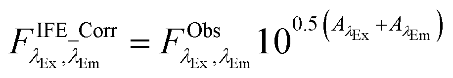 | (3) |
Subsequently, for both rd and rp, the fluorescence data were translated into fDOM attenuation [%] (i.e. percentage difference between pre- and post-correction fDOM is reported) and expressed as a function of Abs254 or turbidity (rd, rp in eqn (2a) and (b)). For instance, an attenuation of 20% translates into a rd of 0.8, i.e. no attenuation is expressed by a rd of 1. The fDOMcorr was calculated according to eqn (2b).
Finally, a DOC model was obtained by linear regression between fDOMcorr and observed DOC concentrations. The DOC concentrations estimated from the fDOMcorr measurements are referred to as DOCfDOM.
The significance of trends of fluorescence indices based on a significance level of 0.05 was evaluated using the Mann–Kendall test,54 which is a non-parametric test known for giving robust results for evaluating temporal trends in water quality-related parameters.55,56
3. Results
3.1. DOC concentrations and character measured in the laboratory
Dry conditions were present for most of the study period, with 304 mm of precipitation from May to September producing an average flow of 1.6 m3 s−1. The precedent snow melt episode led to a maximum discharge of 11.6 m3 s−1 on March 23rd, whereas a rain storm at the end of October (28th) produced a maximum discharge of 16.1 m3 s−1 (Fig. 2). These values are comparably small in relation to long-term average flow data of 13.8 m3 s−1. DOC concentrations followed the discharge pattern (Fig. 2) with highest concentrations in October (up to 26.5 mg L−1) and stable conditions during the summer period (at around 13.5 mg L−1).Optical indices derived from laboratory measurements are presented in Table 2. HIX was the first to reach near-maximum values towards the end of the discharge snow melt peak, directly followed by FI and SUVA. Simultaneously, the T/C ratio and β:α decreased to (near-) minimum values as they are inversely correlated to the aforementioned indices. During the low-flow and low-precipitation months of May to September, significant negative trends (Mann–Kendall test at α = 0.05) were observed for SUVA (p = 0.0163, slope = −0.004 d−1) and HIX (p = 0.0069, slope = −0.0001 d−1) and a positive trend for β:α (p = 0.0027, slope = 0.0006 d−1). During the storm in mid-October, HIX, FI, SUVA and T/C peak changed concurrently to the DOC concentration and reached extreme values (either maximum or minimum depending on the index).
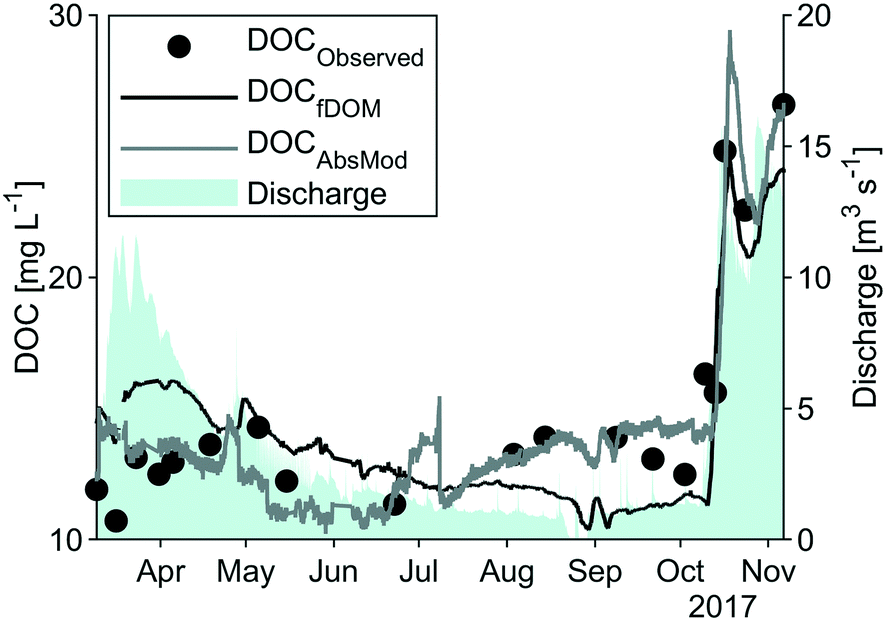 | ||
| Fig. 2 Time series (March to November 2017) of discharge measurements, DOC concentrations of grab samples analysed in the laboratory (DOCObserved) and estimated DOC concentrations based on the fDOM and spectrolyser measurements in the Fyris river. | ||
:α) were calculated from laboratory fluorescence measurements of grab samples from Storvad, as well as the specific ultraviolet absorbance (SUVA) from laboratory absorbance and DOC concentration measurements. All data, except for the corrected fDOM (fDOMcorr EXO2), estimated DOC concentrations from the fDOM model (DOCfDOM) and estimated DOC concentrations from the spectrolyser model (DOCAbsMod), come from offline grab samples analysed in the laboratory
| Date | HIX | FI |
β:α |
SUVA | DOC [mg L−1] | HSa [mg L−1] | HS/DOC | T/C | fDOM lab [QSU] | fDOMcorr EXO2 [QSU] |
|---|---|---|---|---|---|---|---|---|---|---|
| a Calculated from eqn (1). | ||||||||||
| Mar 09 | 0.94 | 1.50 | 0.57 | 3.34 | 11.9 | 8.7 | 0.73 | 0.26 | 169 | 146 |
| Mar 16 | 0.92 | 1.51 | 0.56 | 3.35 | 10.7 | 8.0 | 0.75 | 0.28 | 156 | 136 |
| Mar 23 | 0.94 | 1.48 | 0.54 | 3.35 | 13.1 | 9.9 | 0.76 | 0.21 | 185 | 170 |
| Mar 31 | 0.93 | 1.47 | 0.54 | 3.85 | 12.5 | 10.3 | 0.82 | 0.22 | 183 | 171 |
| Apr 05 | 0.94 | 1.48 | 0.55 | 3.58 | 13.0 | 10.0 | 0.78 | 0.22 | 180 | 171 |
| Apr 18 | 0.94 | 1.45 | 0.56 | 3.16 | 13.6 | 9.4 | 0.69 | 0.27 | 160 | 147 |
| May 05 | 0.93 | 1.46 | 0.55 | 3.24 | 14.3 | 9.5 | 0.66 | 0.26 | 157 | 147 |
| May 15 | 0.93 | 1.45 | 0.56 | 3.14 | 12.2 | 8.5 | 0.70 | 0.30 | 141 | 132 |
| Jun 22 | 0.91 | 1.06 | 0.59 | 2.96 | 11.4 | 7.6 | 0.67 | 0.41 | 125 | 116 |
| Aug 03 | 0.91 | 1.47 | 0.61 | 2.78 | 13.2 | 8.2 | 0.62 | 0.45 | 126 | 109 |
| Aug 14 | 0.91 | 1.50 | 0.61 | 2.52 | 13.9 | 7.8 | 0.56 | 0.53 | 109 | 106 |
| Sep 08 | 0.90 | 1.50 | 0.64 | 2.28 | 13.9 | 7.2 | 0.52 | 0.46 | 111 | 93 |
| Sep 21 | 0.89 | 1.48 | 0.64 | 2.60 | 13.1 | 7.6 | 0.58 | 0.48 | 112 | 97 |
| Oct 02 | 0.90 | 1.48 | 0.63 | 2.70 | 12.5 | 7.6 | 0.61 | 0.43 | 118 | 104 |
| Oct 09 | 0.90 | 1.50 | 0.63 | 2.09 | 16.3 | 7.6 | 0.47 | 0.46 | 117 | 100 |
| Oct 13 | 0.93 | 1.54 | 0.59 | 3.23 | 15.6 | 10.8 | 0.69 | 0.25 | 187 | 181 |
| Oct 16 | 0.94 | 1.50 | 0.54 | 3.35 | 24.8 | 17.1 | 0.69 | 0.22 | 301 | 272 |
| Oct 23 | 0.94 | 1.50 | 0.53 | 3.39 | 22.6 | 15.8 | 0.70 | 0.21 | 246 | 248 |
| Nov 06 | 0.95 | 1.51 | 0.51 | 3.34 | 26.6 | 18.2 | 0.68 | 0.18 | 289 | 293 |
| R 2 DOCfDOM | 0.69 | 0.05 | 0.65 | 0.41 | 0.71 | 0.96 | 0.24 | 0.63 | 0.98 | 1.0 |
| R 2 DOCAbsMod | 0.22 | 0.08 | 0.22 | 0.05 | 0.92 | 0.86 | 0.00 | 0.18 | 0.71 | 0.74 |
Calculated HS concentrations ranged from 6.7 to 18.2 mg L−1 with a mean of 9.2 mg L−1. The relative proportion of HS to DOC decreased from ca. 80% during the spring flood period to ca. 50% in September, and then rapidly increased following the autumn discharge peak to ca. 70%.
3.2. Comparisons of observed and estimated DOC concentrations from in situ measurements
High-frequency measurements were collected from March to November with only short interruptions. Power outages and technical problems (e.g. software issues) led to gaps in the spectrolyser time series during March and April. Generally, weather conditions were reflected by the high-frequency measurements with stable observations of turbidity, conductivity and temperature in the months May to September and extreme values of turbidity and fDOMmeas in March and October. Systematic shifts in the data due to periodical manual cleaning were not apparent.As visible in Fig. A4, ESI†, fDOMcorr compares to the pattern of laboratory DOC in spring and autumn, but in contrast to the stable DOC observations from May to September, it decreased steadily (from 160 QSU to 83 QSU) leading to deviations between the two signals. Correlation between measured DOC and the fDOMcorr resulted in a R2 of 0.71 and a RMSE of 2.5 mg L−1 (Fig. 3 and Table 2).
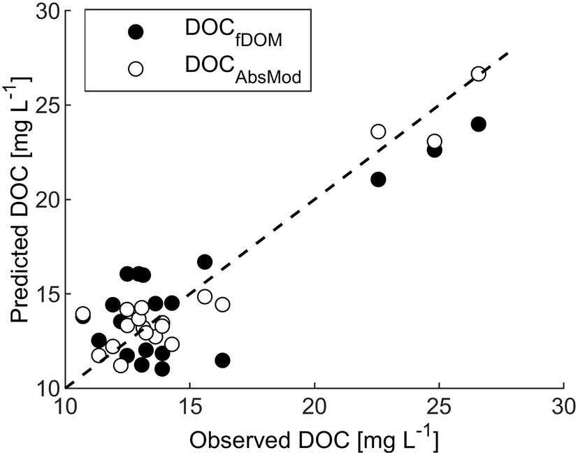 | ||
| Fig. 3 Predicted versus measured DOC for the fDOM and spectrolyser. Dashed line represents the 1:1 line. | ||
Despite the observed trends for the summer period in HIX, SUVA and β:α, none of the indices described well the overall variation in the fDOMcorr signal. HIX (R2 = 0.69) and β:α (R2 = 0.65) correlated better with fDOMcorr than SUVA (R2 = 0.41) and FI (R2 ≤ 0.1). The fDOMcorr deviations were best-explained by the HS concentrations (R2 = 0.96).
:α and SUVA) during the sampling events (all R2 < 0.25, p > 0.01, Table 2), but a significant correlation with HS was apparent (R2 = 0.86, p < 0.001).
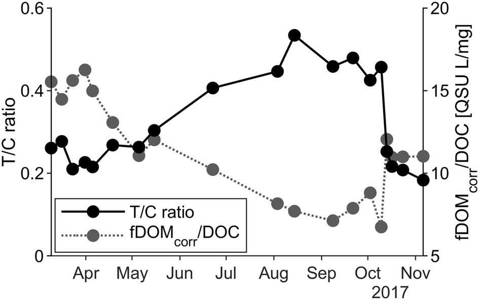 | ||
| Fig. 4 Time series (March to November 2017) of the ratio between the peaks T and C and fDOMcorr/DOC ratio. | ||
4. Discussion
4.1. Sensor evaluation – comparison of DOC estimations
pt?>Both sensors delivered estimates of DOC concentration in the form of high-frequency time series, however, their success at predicting laboratory-based DOC measurement differed. Although both instruments required data post-processing, this was most onerous for the fDOM sensor, which required compensation for temperature, turbidity and IFE, including dedicated experiments to establish sensor- and site-specific corrections. Under the conditions of our study, the spectrolyser resulted in better estimates of DOC concentration than the fDOM sensor. The RMSE for the fDOM sensor estimation (2.5 mg L−1) was greater than that for the spectrolyser (1.3 mg L−1). The absorbance-based DOC model was satisfactory, confirming the suitability of the modelling approach and the stability of the spectrolyser over time. PLS regression from absorbance data has successfully been used previously for calculating DOC concentrations.57,58 On the other hand, in contrast to earlier studies that reported online fDOM to be a reliable proxy for DOC concentration (e.g. R2 = 0.79,59R2 = 0.96,60R2 = 0.93 and 0.8517), we observed a period of relatively poor prediction between May and September.Ruling out errors in setup and data treatment is essential before attempting to explain the differences between observed and estimated DOC by natural processes. Differences between the predictions by the two sensors cannot be explained by instrument setup since flow cell construction and installation were similar for both sensors (Fig. A1, ESI†). Another fDOM sensor installed 9 km downstream at Bärbyleden (Fig. 1), recorded similar fDOM as the one analysed in depth here, as demonstrated by linear correlation with a R2 of 0.99 between the fDOMmeas datasets of the two sensors (data not shown). The fDOM data corrections employed here included a combination of instrument- and site-specific factors, which complicates direct comparisons with other studies that used slightly different approaches in settings with different specific characteristics. However, molecular fluorescence of humic-like organic matter usually drops about 1% °C−1 increase in temperature31,61 and our site-specific temperature correction factor of −0.009 °C−1 matches this and other published values.34,62 Downing et al.32 reported that about 10 to 19% of the fDOM signal was attenuated at a turbidity level of 50 FNU. Our results similarly showed an attenuation of 15% at 50 FNU. Downing et al.32 also reported that correction of the IFE at an absorbance of 0.5 at 254 nm led to about 14 to 28% attenuation. Our correction resulted in an attenuation of 14% at this absorbance. Finally, comparing the field fDOMcorr signal with laboratory fDOM measurements (fDOM lab) from grab samples revealed that, after normalization, the observed dynamics in these two signals were almost identical (R2 = 0.95).
Our results do indicate that the fDOMcorr signal was influenced by changes in DOC character in Fyrisån between March and September. As DOC quantity was stable during long periods of the late spring and summer, we are confident that the measured spectroscopic properties reflected changes in DOC character. The observed trends of HIX, SUVA and β:α from April to September indicate a shift in the DOC quality. During low-flow summer conditions, riverine DOC is composed of less-humified material with a larger contribution of more freshly produced DOC (lower HIX, higher β:α) compared to high-flow conditions. The aromaticity (SUVA) decreased simultaneously and a shift occurred from humic-like (peak C) to protein-like (peak T) organic matter. Underlying reasons are a combination of several processes taking place in both the soil and the water column. On the one hand, during the summer months, low discharge and longer residence times trigger microbial in-stream processes that can lead to the production of microbially-derived DOC. Elevated temperatures enhance microbial activity and the photosynthetic activity of diatoms; evidence of the latter is seen in the decreasing silica concentrations in nearby Klastorp (Fig. A2, ESI†). Similar in-stream processes affecting DOC are typically observed in Mediterranean catchments where dry summer conditions occur frequently.63 On the other hand, a change of the DOC source from the catchment can be considered likely. Our records from the monitoring station at Klastorp indicate that during high discharge, and thus during periods with elevated groundwater tables, absorbance, filtered iron and, consequently, SUVA are increased (Fig. A2 and A6, ESI†), which can be explained by the mobilization of water from shallow riparian soil levels. This is in accordance with the dominant source layer concept.64 At low discharge, groundwater tables are low leading to lateral water inputs from deeper, mineral-like soil layers, which inherit DOC that is less aromatic, more microbially derived, and more recently produced than that from shallow organic riparian layers.20 At deeper soil layers, the character of DOC changes due to the selective removal of terrestrial carbon during soil passage, whereby DOC attaches to mineral surfaces or flocculates with iron or aluminium hydroxides.51
From March to September, we observed lower concentrations of HS and fresher DOC (Table 2), probably due to release of degraded organic matter of the riparian vegetation and from high in-stream processing of fresh organic matter. Changes in the ratio of fDOMcorr per DOC can be a consequence of these processes (Fig. 4). Furthermore, the pattern of the T/C ratio supported the DOC compositional variations. As the signal decreased during the summer months, a shift from the humic-like to the tryptophan-like peak occurred, indicating a shift from allochthonous terrestrial organic matter to autochthonous material, hence greater degree of microbial activity. Monitoring data from the Klastorp site support this conclusion, highlighting the typical annual pattern of high flow, high silica under cold periods and low flow, warm temperature and biological in-stream processing of silica in summer (Fig. A2, ESI†).
We hypothesize that earlier observed good fits between fDOM and DOC were established in surface waters with a smaller fraction of agricultural land use and/or less temporally-variable DOC character, e.g. in lakes32,60,65 that represent more stable environments than our river water. As such, care needs to be taken when using a fDOM sensor for estimating DOC concentrations in lotic waters.
4.2. Application in drinking water treatment
Next to practicalities such as acquisition cost, maintenance and power requirements, the best choice of sensor depends on the monitoring aim and the catchment under investigation. The required accuracy of DOC concentration estimations differs depending on the application of the sensors. For illustration, if during the drinking water production process 3 to 4 mg L−1 were removed, then a DOC estimation error of 1.5 mg L−1 would not be satisfactory. However, for deciding on temporary interruptions of the water intake due to a high concentration event, it might still fulfil its purpose. For drinking water applications, the fDOM sensor might suffice if the main objective is to adjust chemical dose for coagulation processes. The HS, representing the organic matter fraction that can be removed by flocculation,66 showed here a very good correlation with the fDOMcorr (R2 = 0.96). However, complex site- and instrument-specific corrections need to be applied to the data recorded by the fDOM sensor.Grab sampling is also needed in order to maintain the sensors as well as to improve the correction functions. If measurement of several parameters is intended, it might be justified to invest in a full-spectrum sensor and to calibrate it to parameters of interest (e.g. HS fraction, DOC, turbidity). The spectrolyser would be a more reliable choice for predicting DOC, especially in flashy catchments. This study indicates that greater precision in DOC concentration estimates can be achieved if information from a broad range of wavelengths is available as compared to a single excitation sensor.
Sensors offer well-known advantages over intermittent samples, especially the possibility of reacting immediately to changes in the raw water quality, allowing for real-time adjustment of processes such as MAR. Grab samples are prone to miss certain events leading to false assumptions about DOC dynamics, as exemplified here by comparing linearly interpolating DOC concentrations of the grab samples with the estimated DOC concentrations from the spectrolyser, where systematic differences of up to ±4 mg L−1 are present at several periods of days (Fig. A7, ESI†). At drinking water facilities, tracking and responding to changes in DOC character can reduce costs of chemicals and increase membrane lifetimes by reducing backwashing frequency. Once reliable routines for treating sensor data are developed, personnel costs will diminish due to a reduced need for grab samples and laboratory analyses.
5. Conclusions
In this study, a fluorescence- and an absorbance-based sensor were evaluated in relation to their accuracy for estimating DOC concentrations and in their applicability for drinking water production. Both sensors were found to be suitable supportive tools for MAR depending on the water quality parameters of greatest interest at the treatment plant.Optical indices derived from grab samples indicated temporal changes in the DOC character throughout the measuring period in this mixed forested and agricultural landscape. These changes impacted the accuracy of the compared sensors differently. The EXO2 fDOM sensor provided periodically inaccurate predictions of DOC; however, if the objective is to monitor the easily-removed DOC fraction (i.e. HS), then the fDOM sensor is a suitable solution assuming that a convenient post-processing data pipeline can be developed. Further confirmation of the stability of the fDOM–HS relationship is needed. In contrast, the multiple-wavelength model based on spectrolyser absorbance spectra reliably compensated for changes in DOC composition. Expanding the dataset to measure more data under extreme conditions will improve the prediction of the full range of DOC concentrations.
Conflicts of interest
There are no conflicts to declare.Acknowledgements
This work was part of two projects supported by VINNOVA (2017-03729) and SVU (SVU 16-103). KRM was supported by the Swedish Research Council for Environment, Agricultural Sciences and Spatial Planning (FORMAS grant 2013-1214). JLJL was supported by the Swedish Research Council (FORMAS grant 2015-1518) and the Spanish Government through a Juan de la Cierva grant (FJCI-2017-32111). We thank the Department of Earth Sciences at Uppsala University for providing water level measurements and the respective discharge curve and Don Pierson for loaning one of the instruments. We thank Uppsala Vatten for providing access to the site and constructive feedback.References
- B. Bates, Z. W. Kundzewicz, S. Wu and J. Palutikof, Climate Change and Water. Technical Paper of the Intergovernmental Panel on Climate Change, IPCC Secr., Geneva, 2008, p. 210 Search PubMed.
- SOU 2007:60, Final report from the Swedish Commission on Climate and Vulnerability, in Sweden facing climate change – threats and opportunities, Swedish Government Official Reports, Stockholm, 2007 Search PubMed.
- H. A. De Wit, S. Valinia, G. A. Weyhenmeyer, M. N. Futter, P. Kortelainen, K. Austnes, D. O. Hessen, A. Räike, H. Laudon and J. Vuorenmaa, Current Browning of Surface Waters Will Be Further Promoted by Wetter Climate, Environ. Sci. Technol. Lett., 2016, 3, 430–435, DOI:10.1021/acs.estlett.6b00396.
- C. D. Evans, T. G. Jones, A. Burden, N. Ostle, P. Zieliński, M. D. A. Cooper, M. Peacock, J. M. Clark, F. Oulehle, D. Cooper and C. Freeman, Acidity controls on dissolved organic carbon mobility in organic soils, Glob. Change Biol., 2012, 18, 3317–3331, DOI:10.1111/j.1365-2486.2012.02794.x.
- N. Roulet and T. R. Moore, Browning the waters, Nature, 2006, 444, 283–284, DOI:10.1038/444283a.
- N. Her, G. Amy, J. Chung, J. Yoon and Y. Yoon, Characterizing dissolved organic matter and evaluating associated nanofiltration membrane fouling, Chemosphere, 2008, 70, 495–502, DOI:10.1016/j.chemosphere.2007.06.025.
- M.-G. Kang, Y.-H. Ku, Y.-K. Cho and M.-J. Yu, Variation of dissolved organic matter and microbial regrowth potential through drinking water treatment processes, Water Sci. Technol.: Water Supply, 2006, 6, 57–66, DOI:10.2166/ws.2006.904.
- M. J. Nieuwenhuijsen, J. Grellier, R. Smith, N. Iszatt, J. Bennett, N. Best and M. Toledano, The epidemiology and possible mechanisms of disinfection by-products in drinking water, Philos. Trans. R. Soc., A, 2009, 367, 4043–4076, DOI:10.1098/rsta.2009.0116.
- S. Richardson, M. Plewa, E. Wagner, R. Schoeny and D. Demarini, Occurrence, genotoxicity, and carcinogenicity of regulated and emerging disinfection by-products in drinking water: A review and roadmap for research, Mutat. Res., 2007, 636, 178–242, DOI:10.1016/j.mrrev.2007.09.001.
- L. E. Anderson, W. H. Krkošek, A. K. Stoddart, B. F. Trueman and G. A. Gagnon, Lake Recovery Through Reduced Sulfate Deposition: A New Paradigm for Drinking Water Treatment, Environ. Sci. Technol., 2017, 51, 1414–1422, DOI:10.1021/acs.est.6b04889.
- A. Keucken, G. Heinicke, K. Persson and S. Köhler, Combined Coagulation and Ultrafiltration Process to Counteract Increasing NOM in Brown Surface Water, Water, 2017, 9, 697, DOI:10.3390/w9090697.
- N. M. Kortelainen and J. A. Karhu, Tracing the decomposition of dissolved organic carbon in artificial groundwater recharge using carbon isotope ratios, Appl. Geochem., 2006, 21, 547–562, DOI:10.1016/j.apgeochem.2006.01.004.
- P. Baveye, P. Vandevivere, B. L. Hoyle, P. C. DeLeo and D. Sanchez De Lozada, Environmental impact and mechanisms of the biological clogging of saturated soils and aquifer materials, Crit. Rev. Environ. Sci. Technol., 1998, 28, 123–191, DOI:10.1080/10643389891254197.
- K. H. Knorr, DOC-dynamics in a small headwater catchment as driven by redox fluctuations and hydrological flow paths – Are DOC exports mediated by iron reduction/oxidation cycles?, Biogeosciences, 2013, 10, 891–904, DOI:10.5194/bg-10-891-2013.
- E. E. Lavonen, D. N. Kothawala, L. J. Tranvik, M. Gonsior, P. Schmitt-Kopplin and S. J. Köhler, Tracking changes in the optical properties and molecular composition of dissolved organic matter during drinking water production, Water Res., 2015, 85, 286–294, DOI:10.1016/j.watres.2015.08.024.
- D. M. McKnight, E. W. Boyer, P. K. Westerhoff, P. T. Doran, T. Kulbe and D. T. Andersen, Spectrofluorometric characterization of dissolved organic matter for indication of precursor organic material and aromaticity, Limnol. Oceanogr., 2001, 46, 38–48, DOI:10.4319/lo.2001.46.1.0038.
- Y. Shutova, A. Baker, J. Bridgemann and R. K. Henderson, On-line monitoring of organic matter concentrations and character in drinking water treatment systems using fluorescence spectroscoy, Environ. Sci.: Water Res. Technol., 2016, 2, 749–760 RSC.
- J. Wasswa, N. Mladenov and W. Pearce, Assessing the potential of fluorescence spectroscopy to monitor contaminants in source waters and water reuse systems, Environ. Sci.: Water Res. Technol., 2019, 5(2), 370–382 RSC.
- J. L. Weishaar, G. R. Aiken, B. A. Bergamaschi, M. S. Fram, R. Fujii and K. Mopper, Evaluation of specific ultraviolet absorbance as an indicator of the chemical composition and reactivity of dissolved organic carbon, Environ. Sci. Technol., 2003, 37, 4702–4708, DOI:10.1021/es030360x.
- J. L. J. Ledesma, D. N. Kothawala, P. Bastviken, S. Maehder, T. Grabs and M. N. Futter, Stream Dissolved Organic Matter Composition Reflects the Riparian Zone, Not Upslope Soils in Boreal Forest Headwaters, Water Resour. Res., 2018, 54, 3896–3912, DOI:10.1029/2017WR021793.
- K. R. Murphy, C. A. Stedmon, T. D. Waite and G. M. Ruiz, Distinguishing between terrestrial and autochthonous organic matter sources in marine environments using fluorescence spectroscopy, Mar. Chem., 2008, 108, 40–58, DOI:10.1016/j.marchem.2007.10.003.
- C. A. Stedmon, S. Markager and R. Bro, Tracing dissolved organic matter in aquatic environments using a new approach to fluorescence spectroscopy, Mar. Chem., 2003, 82, 239–254, DOI:10.1016/S0304-4203(03)00072-0.
- A. Stubbins, J. F. Lapierre, M. Berggren, Y. T. Prairie, T. Dittmar and P. A. Del Giorgio, What's in an EEM? Molecular signatures associated with dissolved organic fluorescence in boreal Canada, Environ. Sci. Technol., 2014, 48, 10598–10606, DOI:10.1021/es502086e.
- P. J. Hernes, B. A. Bergamaschi, R. S. Eckard and R. G. M. Spencer, Fluorescence-based proxies for lignin in freshwater dissolved organic matter, J. Geophys. Res.: Space Phys., 2009, 114, G00F03, DOI:10.1029/2009JG000938.
- S. A. Huber, A. Balz, M. Abert and W. Pronk, Characterisation of aquatic humic and non-humic matter with size-exclusion chromatography – organic carbon detection – organic nitrogen detection (LC-OCD-OND), Water Res., 2011, 45, 879–885, DOI:10.1016/j.watres.2010.09.023.
- P. Bose and D. A. Reckhow, The effect of ozonation on natural organic matter removal by alum coagulation, Water Res., 2007, 41, 1516–1524, DOI:10.1016/j.watres.2006.12.027.
- M. Edwards, Predicting DOC removal during enhanced coagulation, J. - Am. Water Works Assoc., 1997, 89, 78–89, DOI:10.1002/j.1551-8833.1997.tb08229.x.
- S. J. Köhler, E. Lavonen, A. Keucken, P. Schmitt-Kopplin, T. Spanjer and K. Persson, Upgrading coagulation with hollow-fibre nanofiltration for improved organic matter removal during surface water treatment, Water Res., 2016, 89, 232–240, DOI:10.1016/j.watres.2015.11.048.
- C. R. O'Melia, W. C. Becker and K. K. Au, Removal of humic substances by coagulation, Water Sci. Technol., 1999, 40, 47–54, DOI:10.1016/S0273-1223(99)00639-3.
- H. Laudon, M. Berggren, A. Ågren, I. Buffam, K. Bishop, T. Grabs, M. Jansson and S. J. Köhler, Patterns and Dynamics of Dissolved Organic Carbon (DOC) in Boreal Streams: The Role of Processes, Connectivity, and Scaling, Ecosystems, 2011, 14, 880–893, DOI:10.1007/s10021-011-9452-8.
- A. Baker, Thermal fluorescence quenching properties of dissolved organic matter, Water Res., 2005, 39, 4405–4412, DOI:10.1016/j.watres.2005.08.023.
- B. D. Downing, B. A. Pellerin, B. A. Bergamaschi, J. F. Saraceno and T. E. C. Kraus, Seeing the light: The effects of particles, dissolved materials, and temperature on in situ measurements of DOM fluorescence in rivers and streams, Limnol. Oceanogr.: Methods, 2012, 10, 767–775, DOI:10.4319/lom.2012.10.767.
- J. F. Saraceno, J. B. Shanley, B. D. Downing and B. A. Pellerin, Clearing the waters : Evaluating the need for site-specific field fluorescence corrections based on turbidity measurements, Limnol. Oceanogr.: Methods, 2017, 15, 408–416, DOI:10.1002/lom3.10175.
- C. J. Watras, P. C. Hanson, T. L. Stacy, K. M. Morrison, J. Mather, Y.-H. Hu and P. Milewski, A temperature compensation method for CDOM fluorescence sensors in freshwater, Limnol. Oceanogr.: Methods, 2011, 9, 296–301, DOI:10.4319/lom.2011.9.296.
- K. Khamis, J. P. R. Sorensen, C. Bradley, D. M. Hannah, D. J. Lapworth and R. Stevens, In situ tryptophan-like fluorometers: assessing turbidity and temperature effects for freshwater applications, Environ. Sci.: Processes Impacts, 2015, 17, 740–752, 10.1039/c5em00030k.
- G. de Oliveira, E. Bertone, R. Stewart, J. Awad, A. Holland, K. O'Halloran and S. Bird, Multi-Parameter Compensation Method for Accurate In Situ Fluorescent Dissolved Organic Matter Monitoring and Properties Characterization, Water, 2018, 10, 1146, DOI:10.3390/w10091146.
- J. L. J. Ledesma, S. J. Köhler and M. N. Futter, Long-term dynamics of dissolved organic carbon: Implications for drinking water supply, Sci. Total Environ., 2012, 432, 1–11, DOI:10.1016/j.scitotenv.2012.05.071.
- L. Gottschalk, J. L. Jensen, D. Lundquist, R. Solantie and A. Tollan, Hydrologic Regions in the Nordic Countries, Hydrol. Res., 1979, 10, 273–286 CrossRef.
- J. F. Exbrayat, N. R. Viney, J. Seibert, S. Wrede, H. G. Frede and L. Breuer, Ensemble modelling of nitrogen fluxes: Data fusion for a Swedish meso-scale catchment, Hydrol. Earth Syst. Sci., 2010, 14, 2383–2397, DOI:10.5194/hess-14-2383-2010.
- HORIBA Instruments Incorporated, AquaLog Operational Manual., Rev. B, 2012 Search PubMed.
- A. J. Lawaetz and C. A. Stedmon, Fluorescence Intensity Calibration Using the Raman Scatter Peak of Water, Appl. Spectrosc., 2009, 63, 936–940, DOI:10.1366/000370209788964548.
- YSI Incorporated, a Xylem brand, EXO2: EXO User Manual ADVANCED WATER QUALITY MONITORING PLATFORM, 2017 Search PubMed.
- s::can Messtechnik GmbH, S::can spectrometer probe: Manual s::can spectrometer probe, 2007 Search PubMed.
- J. Fölster, R. K. Johnson, M. N. Futter and A. Wilander, The Swedish monitoring of surface waters: 50 years of adaptive monitoring, Ambio, 2014, 43, 3–18, DOI:10.1007/s13280-014-0558-z.
- T. Ohno, Fluorescence inner-filtering correction for determining the humification index of dissolved organic matter, Environ. Sci. Technol., 2002, 36, 742–746, DOI:10.1021/es0155276.
- R. M. Cory and D. M. McKnight, Fluorescence Spectroscopy Reveals Ubiquitous Presence of Oxidized and Reduced Quinones in Dissolved Organic Matter, Environ. Sci. Technol., 2005, 39, 8142–8149, DOI:10.1021/es0506962.
- E. Parlanti, K. Wörz, L. Geoffroy and M. Lamotte, Dissolved organic matter fluorescence spectroscopy as a tool to estimate biological activity in a coastal zone submitted to anthropogenic inputs, Org. Geochem., 2000, 31, 1765–1781, DOI:10.1016/S0146-6380(00)00124-8.
- P. G. Coble, Characterization of marine and terrestrial DOM in seawater using excitation-emission matrix spectroscopy, Mar. Chem., 1996, 51, 325–346, DOI:10.1016/0304-4203(95)00062-3.
- Grundvattengruppen for Uppsala Vatten, Uppsala Vatten report, in Funktionanalys Uppsalaåsen, Uppsala, 2017 Search PubMed.
- J. R. Lakowicz, in Principles of Fluorescence Spectroscopy, ed. J. R. Lakowicz, Springer US, Boston, MA, 3rd edn, 2006, DOI:10.1007/978-0-387-46312-4.
- D. N. Kothawala, K. R. Murphy, C. A. Stedmon, G. A. Weyhenmeyer and L. J. Tranvik, Inner filter correction of dissolved organic matter fluorescence, Limnol. Oceanogr.: Methods, 2013, 11, 616–630, DOI:10.4319/lom.2013.11.616.
- L. Eriksson, E. Johansson and S. Wold, Introduction to Multi- and Megavariate Data Analysis Using Projection Methods (PCA & PLS), Umetrics AB, 1999 Search PubMed.
- L. M. Carrascal, I. Galván and O. Gordo, Partial least squares regression as an alternative to current regression methods used in ecology, Oikos, 2009, 118, 681–690, DOI:10.1111/j.1600-0706.2008.16881.x.
- H. B. Mann, Nonparametric Tests Against Trend, Econometrica, 1945, 13, 245–259, DOI:10.2307/1907187.
- C. D. Evans, D. T. Monteith and D. M. Cooper, Long-term increases in surface water dissolved organic carbon: Observations, possible causes and environmental impacts, Environ. Pollut., 2005, 137, 55–71, DOI:10.1016/j.envpol.2004.12.031.
- A. Prechtel, C. Alewell, M. Armbruster, J. Bittersohl, J. M. Cullen, C. D. Evans, R. Helliwell, J. Kopácek, A. Marchetto, E. Matzner, H. Meesenburg, F. Moldan, K. Moritz, J. Veselý and R. F. Wright, Response of sulphur dynamics in European catchments to decreasing sulphate deposition, Hydrol. Earth Syst. Sci., 2001, 5, 311–326, DOI:10.5194/hess-5-311-2001.
- J. R. Etheridge, F. Birgand, J. A. Osborne, C. L. Osburn, M. R. Burchell and J. Irving, Using in situ ultraviolet-visual spectroscopy to measure nitrogen, carbon, phosphorus, and suspended solids concentrations at a high frequency in a brackish tidal marsh, Limnol. Oceanogr.: Methods, 2014, 12, 10–22, DOI:10.4319/lom.2014.12.10.
- M. C. H. Vaughan, W. B. Bowden, J. B. Shanley, A. Vermilyea, R. Sleeper, A. J. Gold, S. M. Pradhanang, S. P. Inamdar, D. F. Levia, A. S. Andres, F. Birgand and A. W. Schroth, High-frequency dissolved organic carbon and nitrate measurements reveal differences in storm hysteresis and loading in relation to land cover and seasonality, Water Resour. Res., 2017, 53, 5345–5363, DOI:10.1002/2017WR020491.
- J. T. Crawford, L. C. Loken, N. J. Casson, C. Smith, A. G. Stone and L. A. Winslow, High-speed limnology: Using advanced sensors to investigate spatial variability in biogeochemistry and hydrology, Environ. Sci. Technol., 2015, 49, 442–450, DOI:10.1021/es504773x.
- J. F. Saraceno, B. A. Pellerin, B. D. Downing, E. Boss, P. A. M. Bachand and B. A. Bergamaschi, High-frequency in situ optical measurements during a storm event: Assessing relationships between dissolved organic matter, sediment concentrations, and hydrologic processes, J. Geophys. Res.: Biogeosci., 2009, 114, 1–11, DOI:10.1029/2009JG000989.
- A. Vodacek and W. D. Philpot, Environmental effects on laser-induced fluorescence spectra of natural waters, Remote Sens. Environ., 1987, 21, 83–95, DOI:10.1016/0034-4257(87)90008-3.
- K. Khamis, C. Bradley, R. Stevens and D. M. Hannah, Continuous field estimation of dissolved organic carbon concentration and biochemical oxygen demand using dual-wavelength fluorescence, turbidity and temperature, Hydrol. Processes, 2017, 540–555, DOI:10.1002/hyp.11040.
- S. Bernal, A. Lupon, N. Catalán, S. Castelar and E. Martí, Decoupling of dissolved organic matter patterns between stream and riparian groundwater in a headwater forested catchment, Hydrol. Earth Syst. Sci., 2018, 22, 1897–1910, DOI:10.5194/hess-22-1897-2018.
- J. L. J. Ledesma, M. N. Futter, M. Blackburn, F. Lidman, T. Grabs, R. A. Sponseller, H. Laudon, K. H. Bishop and S. J. Köhler, Towards an Improved Conceptualization of Riparian Zones in Boreal Forest Headwaters, Ecosystems, 2018, 21, 297–315, DOI:10.1007/s10021-017-0149-5.
- E. J. Lee, G. Y. Yoo, Y. Jeong, K. U. Kim, J. H. Park and N. H. Oh, Comparison of UV-VIS and FDOM sensors for in situ monitoring of stream DOC concentrations, Biogeosciences, 2015, 12, 3109–3118, DOI:10.5194/bg-12-3109-2015.
- E. L. Sharp, S. A. Parsons and B. Jefferson, The impact of seasonal variations in DOC arising from a moorland peat catchment on coagulation with iron and aluminium salts, Environ. Pollut., 2006, 140, 436–443, DOI:10.1016/j.envpol.2005.08.001.
Footnote |
| † Electronic supplementary information (ESI) available. See DOI: 10.1039/d0ew00150c |
| This journal is © The Royal Society of Chemistry 2020 |