
 Open Access Article
 This Open Access Article is licensed under a Creative Commons Attribution-Non Commercial 3.0 Unported Licence
Reduction of 1,2,3-trichloropropane (TCP): pathways and mechanisms from computational chemistry calculations†
Tifany L.
Torralba-Sanchez
 a,
Eric J.
Bylaska
b,
Alexandra J.
Salter-Blanc
c,
Douglas E.
Meisenheimer
a,
Molly A.
Lyon
a and
Paul G.
Tratnyek
*a
a,
Eric J.
Bylaska
b,
Alexandra J.
Salter-Blanc
c,
Douglas E.
Meisenheimer
a,
Molly A.
Lyon
a and
Paul G.
Tratnyek
*a
aOHSU-PSU School of Public Health, Oregon Health & Science University, 3181 SW Sam Jackson Park Road, Portland, OR 97239, USA. E-mail: tratnyek@ohsu.edu; Tel: +1-503-346-3431
bWilliam R. Wiley Environmental Molecular Sciences Laboratory, Pacific Northwest National Laboratory, P.O. Box 999, Richland, WA 99352, USA
cJacobs, 2020 SW 4th Avenue, Suite 300, Portland, OR 97201, USA
First published on 23rd January 2020
Abstract
The characteristic pathway for degradation of halogenated aliphatic compounds in groundwater or other environments with relatively anoxic and/or reducing conditions is reductive dechlorination. For 1,2-dihalocarbons, reductive dechlorination can include hydrogenolysis and dehydrohalogenation, the relative significance of which depends on various structural and energetic factors. To better understand how these factors influence the degradation rates and products of the lesser halogenated hydrocarbons (in contrast to the widely studied per-halogenated hydrocarbons, like trichloroethylene and carbon tetrachloride), density functional theory calculations were performed to compare all of the possible pathways for reduction and elimination of 1,2,3-trichloropropane (TCP). The results showed that free energies of each species and reaction step are similar for all levels of theory, although B3LYP differed from the others. In all cases, the reaction coordinate diagrams suggest that β-elimination of TCP to allyl chloride followed by hydrogenolysis to propene is the thermodynamically favored pathway. This result is consistent with experimental results obtained using TCP, 1,2-dichloropropane, and 1,3-dichloropropane in batch experiments with zerovalent zinc (Zn0, ZVI) as a reductant.
Environmental significanceAmong the many halocarbons of environmental concern, 1,2,3-trichloropropane (TCP) is an extreme case because of its very high toxicity and persistence. Recently intensified monitoring for TCP in California has identified low but concerning concentrations in groundwater used for drinking water supplies in agricultural regions where soil fumigants containing TCP were widely used. The current method for treating TCP contaminated water supplies is adsorption on carbon-based filters, but a treatment processes that degrades TCP would be more desirable. While TCP is recalcitrant to degradation by most pathways under most conditions, an energetically favorable pathway to complete dechlorination is available. |
1. Introduction
Most halogenated aliphatic chemicals (alkyl halides) of environmental concern are C1–C3 alkanes and alkenes. Some members of this class of contaminants have been studied extensively over many years—e.g., trichloroethylene (TCE)—while others are contaminants of emerging concern on which there has been relatively little study of their environmental fate or effects. A prominent example of the latter group is 1,2,3-trichloropropane (TCP), which was assigned a maximum contaminant level (MCL) of 5 ppt by the State of California in 2017.1 This extraordinarily low MCL was based on evidence that TCP is carcinogenic,2 and triggered by discovery of TCP contamination in wells that supply drinking water to multiple communities across California.3 Other states have also found TCP in their water and have established MCLs. TCP was identified in Hawaii as early as the 1980s (ref. 4) and the state established an MCL of 0.6 μg L−1 in 2005.5,6 New Jersey established an MCL of 0.03 ppb in 2018.7,8The risk posed by potential human exposure to such a toxic chemical is compounded by TCP's overall resistance to biotic and abiotic processes that contribute to natural attenuation of other alkyl halides in groundwater.9,10 Remediation or treatment of waters contaminated with TCP can be accomplished by sorption (e.g. to activated carbon),11 which is the method most often used for drinking water treatment,5,12,13 however, adsorption of TCP to GAC (granular activated carbon) is generally less favorable than other chlorinated solvents.14 Air stripping, air sparging, and soil vacuum extraction are also less effective compared to other VOCs (volatile organic compounds)15 because of TCP's relatively low Henry's Law constant.16 In general, degradation to benign products would be preferred, but efforts to demonstrate TCP degradation using treatment methods commonly used for other alkyl halides have found that TCP is exceptionally recalcitrant.9,15,17 This challenge has led to exploration of an increasingly diverse and innovative variety of treatment processes for TCP, including novel microbial isolates,18–21 engineered enzymes and microorganisms,10,22–25 chemical reduction using zerovalent zinc,9,26–28 vitamin B12 mediated reduction with zerovalent iron (ZVI),29 chemical oxidation with persulfate,28,30 and alkaline hydrolysis with ammonia.31
The generally low reactivity and high persistence of TCP—especially under anoxic or reducing conditions—is typical of alkyl halides with few halogens per carbon: i.e., “lesser halogenated hydrocarbons” (LHHCs). This is evident in recent work with the closest homologue to TCP, which is 1,2-dichloropropane (DCP).29,32,33 Other relevant LHHCs include 1,2-dichloroethane (ethylene dichloride, EDC), 1,2-dibromoethane (ethylene dibromide, EDB), 1-bromopropane (n-propyl bromide, nPB), 1,2-dibromo-3-chloropropane (DBCP), cis- and trans-1,2-dichloroethene (DCEs), and vinyl chloride (VC). Many of these LHHCs are characterized by single halogens on adjacent sp3 hybridized carbons. These moieties comprise all of the backbone of TCP, which makes it a potential model for the degradation of other LHHCs. While the focus of this study is on TCP, the scope was designed to include other related LHHCs in order to demonstrate similarities and differences in the reactivity of members of this class of chemicals.
In principle, dechlorination of TCP under reducing conditions can occur by any of the first four reactions summarized in Fig. 1.34–36 Two of these are non-redox reactions: nucleophilic substitution (NuS) by H2O/OH− (i.e., hydrolysis) or by sulfide species and dehydrohalogenation (DHX). The two redox reactions are hydrogenolysis (HGL) and reductive β-elimination (BRE). These reactions, together with hydrogenation (HDG) of the alkenes formed by BRE and DHX, should be sufficient to explain all of the products formed from TCP degradation under most groundwater conditions. Recent evidence suggests that oxidation of some alkyl halides is possible under groundwater conditions due to Fenton-like reactions37–39—and this would produce different products than are shown in Fig. 1—but this pathway was omitted from this study because there currently is no evidence that it is significant under fully anoxic conditions. Several of the overall reactions shown in Fig. 1 could occur by more than one mechanism (e.g., sequential vs. concerted transfer of electrons and protons) and some of these options are discussed later in the work.
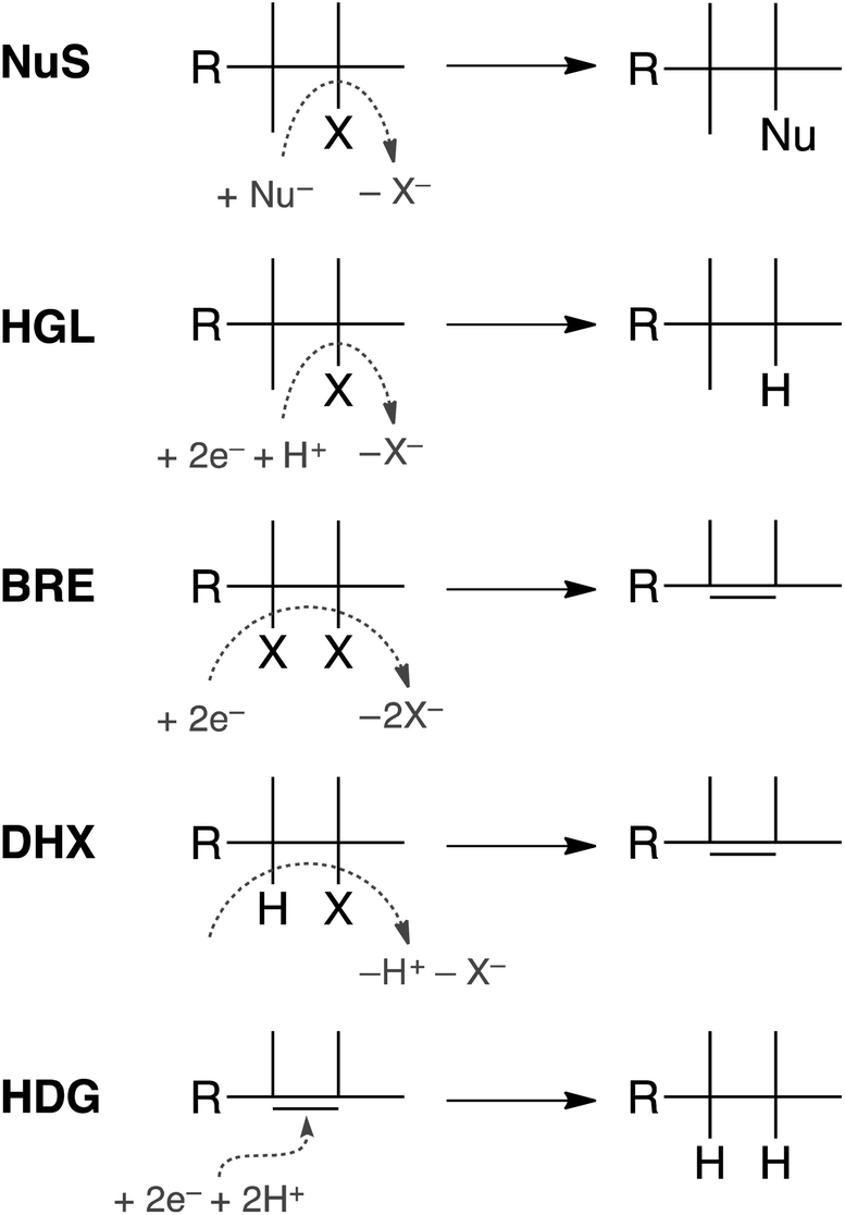 | ||
| Fig. 1 Summary of the main pathways of alkyl halide transformation under reducing conditions. Nu represents the nucleophiles from water or sulfide, X represents any halide including chlorine, e− represents electrons from any reductant, and R represents any alkyl substituent including −CClH3 for TCP. The abbreviations represent common pathway names for each pathway. NuS: nucleophilic substitution, HGL: hydrogenolysis, BRE: reductive β-elimination, DHX: dehydrohalogenation, and HDG: hydrogenation. | ||
In practice, the degradation of TCP under reducing conditions is likely to be controlled by a small subset of the possible reactions summarized in Fig. 1. The relative rates of these reactions will determine the concentrations of intermediate and final reaction products; and these rates will be controlled by properties of the contaminant-derived species, any environmental species involved in the reaction (e.g., reductants), and medium conditions such as pH and temperature. Furthermore, the environmental factors (reductant speciation and concentration, pH, etc.) often vary with space and time, and generally are not well know. Therefore, the only way to know the overall result of contaminant transformation is to directly measure it under realistic environmental conditions. Direct measurement has limitations, however, which include inaccuracies due to experimental error, inefficiencies due to the need for seperate experiments at each combination of conditions, datagaps involving species that are not directly measureable, and ambiguities in interpretation because experimental results can be influenced by factors that are not known or well-understood. These limitations become less significant as the number of experimental studies becomes large, but they are major concerns for less-well studied contaminants like TCP.
The main alternative to experimental measurement for characterization of alternative reaction pathways is to use computational chemistry methods to calculate reaction pathway energetics and kinetics from electronic structure theory.40–44 The advantages and disadvantages of the computational approach are complementary to those of the experimental approach, so they are best pursued in parallel. With respect to TCP degradation, the only previous study to take the computational approach45 used a variety of intermediate levels of theory and standard solvation models to show that the thermodynamically most favorable reaction at STP was reductive β-elimination, followed closely by hydrogenolysis, dehydrochlorination, and hydrolysis. However, this study was limited in that it only considered a small number of reactions without considering multi-step reaction pathway energetics and kinetics. Not surprisingly, conclusions from this previous study are not entirely consistent with experimental data that has since been reported, which show that reactivity of TCP is characterized by being slow and selective under mostly conditions. To reconcile these results, this paper applies higher levels of computational theory to determine the free energies of a wider range of reactions involving TCP and related LHHCs. The results are summarized as reaction coordinate diagrams using a method that efficiently plots the diagrams from tabulated reaction energy data. Comparing reaction coordinate diagrams obtained at different levels of theory shows that all of the higher-level theories predict the observed pathway of slow TCP reduction by BRE followed by rapid HGL to completely dechlorinated products.
2. Methods
2.1. Computational methods
In previous work,46,47 we compared the performance of several electronic structure methods (functionals, basis sets, and solvation models) for computation of one-electron oxidation potentials (E1,ox) for aromatic amines, phenols, and anilines, and a selection of those methods was used in this study. Electronic structure methods were used here for the computation of gas and aqueous phase reaction energies for three major transformation pathways of TCP, viz. HGL, DHX, and BRE + HDG. All of the necessary electronic structure calculations were performed using the NWChem program suite (Version 6.8)48 through Arrows, a new open access scientific service that facilitates running molecular modeling codes at EMSL (Environmental Molecular Science Laboratory, Richland, WA) via a Web API (Application Programing Interface).49 The calculations were performed using both density functional theory (DFT)50,51 and the prefered WFT-based (wave function theory) method52 CCSD(T), coupled cluster single-double (triple).53,54 Previous studies have also benchmarked results between DFT and high-level WFT-based methods for the reactivity of other substances of environmental concern including alkyl halides and aromatic compounds.55,56 For small molecules, CCSD(T) and its variants is considered the most accurate many-body quantum chemistry method in use today.57–60 The basis set we used here was 6-311++G(2d,2p),57,61 and the exchange-correlation functionals (xcFncs) used for DFT were B3LYP,58,62 PBE0,63 PBE96,64 and M06-2X.65 Aqueous phase solvation energies were estimated using the self-consistent reaction field theory of Klamt and Schüürmann (COSMO, COnductor-like Screening MOdel).66 Additional details regarding the computation methods are given in ESI.†3. Results and discussion
3.1. Preliminary assessment of relevant reaction network
To direct the modeling performed in this study, a systematic reaction network was developed of all the most likely steps in degradation of TCP under reducing conditions. This scheme (Fig. 2) was based on (i) the general pathways of alkyl halide transformation that are summarized in Fig. 1 and (ii) the three reaction pathway schemes specifically for TCP that have been reported previously. The most relevent of the published reaction schemes for TCP is the one developed by Sarathy et al.9—and since adopted in multiple places (e.g.,15)—which presents oxidation, reduction, and elimination reactions arranged according to the “square scheme” conventions for redox reactions of organics.67 The scheme in Bylaska et al.45 is also adapted from the one by Sarathy et al., but is more mechanistically complete because it shows the role of the dichloroallyl radicals as possible intermediates in both hydrogenolysis and reductive elimination pathways. Fig. 2 includes these species (INT1 and INT2) as well as the other analogous intermediates that could play a role in the other reduction and elimination pathways for TCP and its less chlorinated congeners. For each of these intermediates, only the doublet radical is included in Fig. 2, because it always was lower in energy (by about 8 kcal mol−1) than the corresponding triplet radical. Another possibility would be intermediates from anchimeric cyclization (such as proposed for vicinal dibromides68), but these radicals for TCP were found to be unstable in solution (modeling not shown).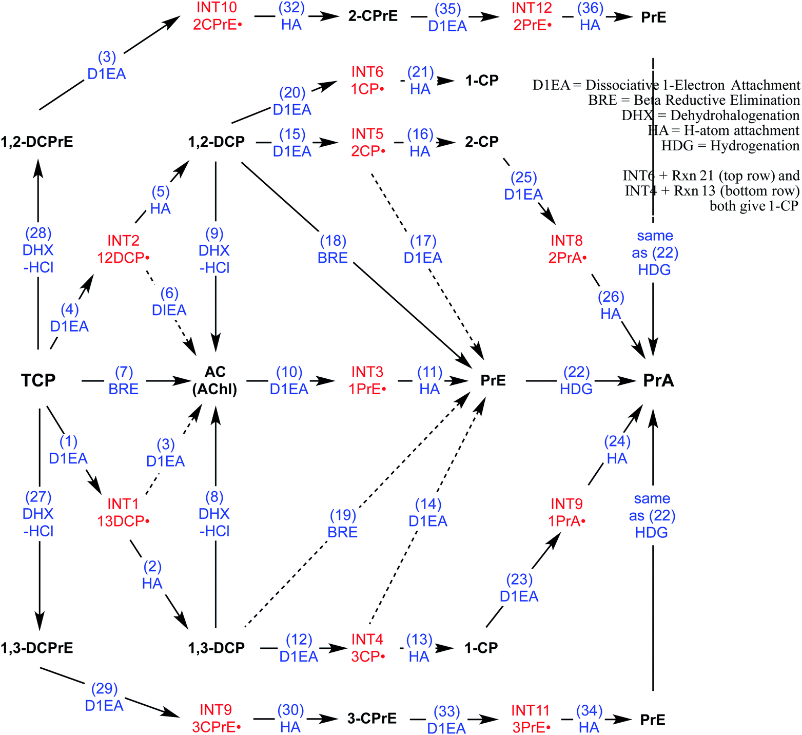 | ||
| Fig. 2 Network of likely reactions for TCP under reducing conditions. Stable reactants and products (bold black text) and radical intermediates (red text) are labelled with abbreviations that are defined in Table S1.† Reaction labels are given by name and number (blue text) defined in Table S1.† Dashed arrows indicate reactions of uncertain likelihood. | ||
Only two major classes of contaminant transformation pathways that might be significant for TCP under some conditions are not included in Fig. 2. One of these classes is nucleophilic substitution (NuS), which is shown only generically in Fig. 1 to allow for replacement of chloride by either O-nucleophiles (hydrolysis) or S-nucleophiles (mainly sulfide species). Some modeling and discussion of hydrolysis reactions was presented in our previous work on TCP.45 NuS reactions involving S-nucleophiles were excluded entirely from the scope of this study—even though products from these reactions have been reported in one study on TCP biodegradation using sulfidic culture media20—because all of our data are from non-sulfidic conditions. The other class not shown involves bridge-stabilized radicals because they were found to be unstable (as noted above).
3.2. Calculation of free energies of reaction steps
The change in standard state Gibbs free energy (ΔG0rxn) provides a quantitative estimate of the thermodynamic feasibility of a reaction. Comparison of ΔG0rxn values among reactions can be used to determine the most energetically favorable transformation pathways. This thermodynamic quantity can be calculated from measured free energy of formation data, but is more efficiently obtained using electronic structure computational methods. Here, these methods were used to perform molecular geometry optimizations followed by electronic energy, frequency, and aqueous phase solvation calculations. The output of these computations for the total electronic energy, entropy, (thermal correction to) enthalpy, and standard state solvation Gibbs free energy for each reaction component were used to calculate the ΔG0rxn values in the aqueous phase, ΔG0rxn(aq), using eqn (1) through (3).| ΔG0rxn(aq) = ΔG0rxn(g) + ΔG0solv | (1) |
 | (2) |
| G0corr = H0corr − TS0tot | (3) |
3.3. Free energies of reaction from different theory levels
A well-known source of differences in calculated ΔG0rxn values for a single reaction is the choice of theory levels (e.g., DFT vs. CCSD(T)) and xcFncs (e.g., B3LYP vs. M06-2X), as they both determine the details by which E0 is computed.69,70 Here, four different functionals were used and compared to calculate the exchange-correlation energies with DFT. The DFT results were also compared against CCSD(T). A comparison of the results obtained with the four different DFT xcFncs is shown in Fig. 3, which contains calculated ΔG0rxn values for selected examples of the TCP transformation pathways presented in Fig. 2. Most of the ΔG0rxn values for individual reactions in Fig. 3 (i.e., columns in each panel) plot as overlapping markers, indicating that differences across xcFncs (and CCSD(T)) are not significant relative to the variability among reactions and, hence, pathways.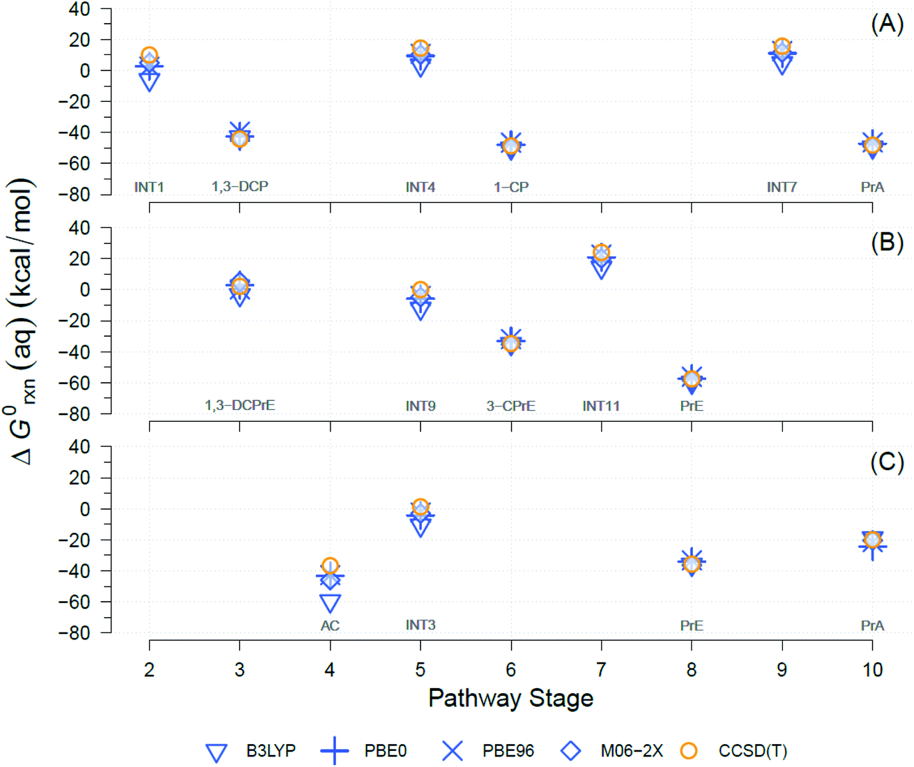 | ||
| Fig. 3 Comparison between theory levels for computationally derived aqueous phase Gibbs free energies (ΔG0rxn(aq), kcal mol−1) of individual reactions for selected TCP transformation pathways shown in Fig. 2. Theory levels: DFT, in blue, and CCSD(T), in yellow. Exchange-correlation functionals for DFT: B3LYP, PBE0, PBE96, and M06-2X. (A) Pathway (1): HGL (trans-branch), (B) pathway (2): DHX (trans-branch), and (C) pathway (3): BRE + HDG. Pathway stage numbers indicate progression of the transformation route and specifically refer to the reaction coordinate (RC) assigned to the main reaction products (see Sections 3.4 and 3.5 for details). RCs and abbreviations listed and defined in Table S1.† H-atom model used: hydron (H+) (see Section 3.3 for details). | ||
Fig. 3 shows that the ΔG0rxn values for individual reactions across all the methods differ little compared with differences among reaction types, with the exception of DFT with B3LYP (e.g., Fig. 3(C) pathway stage (4)). Statistical calculations support these conclusions because the differences in ΔG0rxn across individual reactions have standard deviations ≤±4 kcal mol−1 (standard errors ≤±2 kcal mol−1) and ranges never wider than 9 kcal mol−1. These variabilities are insignificant compared with the 120 kcal mol−1 range (y-axis in Fig. 3) in ΔG0rxn values among the different reactions. These small discrepancies are also within the range seen in our previous work with TCP45 and general comparisons across computational methods.71,72
DFT with the B3LYP exchange-correlation functional is the only method that gives ΔG0rxn values that differ noticeably from the other methods, so including them in statistical calculations would increase standard deviations, standard errors, and ranges mentioned to ≤±8, ≤±4, and 23 kcal mol−1, respectively. In addition, there has been extensive discussion about the difficulties with using B3LYP to model atomic anions (e.g., Cl−) and radicals in proton-coupled electron transfers,73,74 both of which are involved in the majority of the reactions in Fig. 2.
All the DFT methods are in agreement with the presumably more accurate CCSD(T) method, which is the most robust WFT type method currently available.75,76 WFT methods provide a higher level of description of the electronic structure as they render a numerical value for each electron for each point in space, in contrast to DFT methods, which calculate the electronic energy based on the electron density at each point in space. CCSD(T) uses WFT to model the interactions of electrons within small clusters (mostly sets of two) and among those clusters, an approach that has shown to be more computationally intensive than DFT, but with greater performance results.59,77,78 However, DFT continues to be used more frequently than CCSD(T) because, in addition to the lower computational cost, DFT has a significantly more favorable scaling behavior with respect to system size, which is N4vs. N7 for CCSD(T), where N is a relative measure of the number of electrons and atomic orbitals basis functions.44,79 Given the manageable system sizes of the molecules in the proposed TCP transformation network, the similarities in our results between CCSD(T) and most of the DFT functionals, and the superior fundamental accuracy of CCSD(T), we chose to present the following discussion based only on the computations performed with CCSD(T).
In addition to using an experimental value for the solvation energy of hydron (ΔG0solv(H+) ≈ −264 kcal mol−1 (ref. 80)) in the calculation of ΔG0rxn for the H-atom attachment (HA) reactions, we tested a COSMO computed value, i.e., the solvation energy of hydronium with the specified xcFnc (ΔG0solv(H3O+) ≈ −97 kcal mol−1). The trends in ΔG0rxn across the HA reactions were the same regardless of the H-atom solvation energy used, but the experimental H+ yielded less negative (larger) ΔG0rxn for all the reactions (by 10–15 kcal mol−1) as shown in Fig. S1 and Table S3.† We chose to present the following discussion based only on the calculations obtained with the experimental ΔG0solv(H+).
3.4. Calculation of reaction coordinate diagrams
The individual reactions described in the previous section can be arranged in various combinations to represent the possible mechanisms and overall reaction pathways for degradation of TCP. Plotting the sequence of stages on the abcissa (reaction coordinate, RC) vs. the cumulative energy at each stage on the ordinate gives a quantitative reaction coordinate diagram (RCD), which can be a powerful tool for characterization and comparison of reaction pathways. RCDs that only include the free energies of stable species are useful for comparing the energetics of reaction pathways, but they can also include transition states, which then provide insight into reaction barriers and therefore kinetics. Recent examples of RCD interpretation in the literature on contaminant fate include determination of the main decomposition pathways for diverse substances of pressing environmental concern such as insensitive munition compounds81 and PFAS (per- and polyfluoroalkyl substances).82In general, almost all published RCDs appear to be drawings based on qualitative considerations of the relative energies or graphs that are manually compiled. Here, we have developed and applied a code in R software for statistical computing83 that automates the process of translating computationally derived ΔG0rxn values for large and complex networks of transformation pathways to graphed RCDs. This R script along with the corresponding instructions, input, and output files is available for open-access at the Zenodo website.84 Briefly, the R routine reads an input file containing the calculated ΔG0rxn values, which is formatted with five column identifiers per row (viz., identification number (ID), name of the major/main reaction product, RC, RC for the preceding product, and ID for the preceding RC in cases where a single product exists in more than one pathway) with the rows corresponding to the RC assigned to each major reaction product in the transformation pathway. Once this input file is scanned, the R routine maps each of the reactions according to the RCs in ascending order and accumulates the corresponding ΔG0rxn values incrementally at each stage. Once the cumulative ΔG0rxn value at a stage is calculated, it is plotted at the corresponding RC. This process continues along the progress of the pathway and is repeated across all the transformation pathways listed in the input file via a loop in the R routine. The resulting output is a quantitatively accurate graph of an RCD.
3.5. Quantitative comparison of pathways using reaction coordinate diagrams
Using the R routine described above, we built the RCDs for each of the pathways shown in Fig. 2 and overlaid them to accurately determine pathways with the minimum reaction energy requirements as well as to identify intermediates and/or products that demand higher energy inputs. Fig. 4 contains the RCDs for the TCP transformation pathways in Fig. 2, with each of the main reaction mechanisms (i.e., HDG, DHX, and BRE + HDG) as one of the horizontal panels. Fig. 4 only shows ΔG0rxn values derived from CCSD(T) computations; the equivalent RCD comparisons derived from DFT methods are included in the ESI.† While specific ΔG0rxn values varied among methods, energy profiles were very similar and, hence, led to the same conclusions about comparative thermodynamic favorability for the different pathways.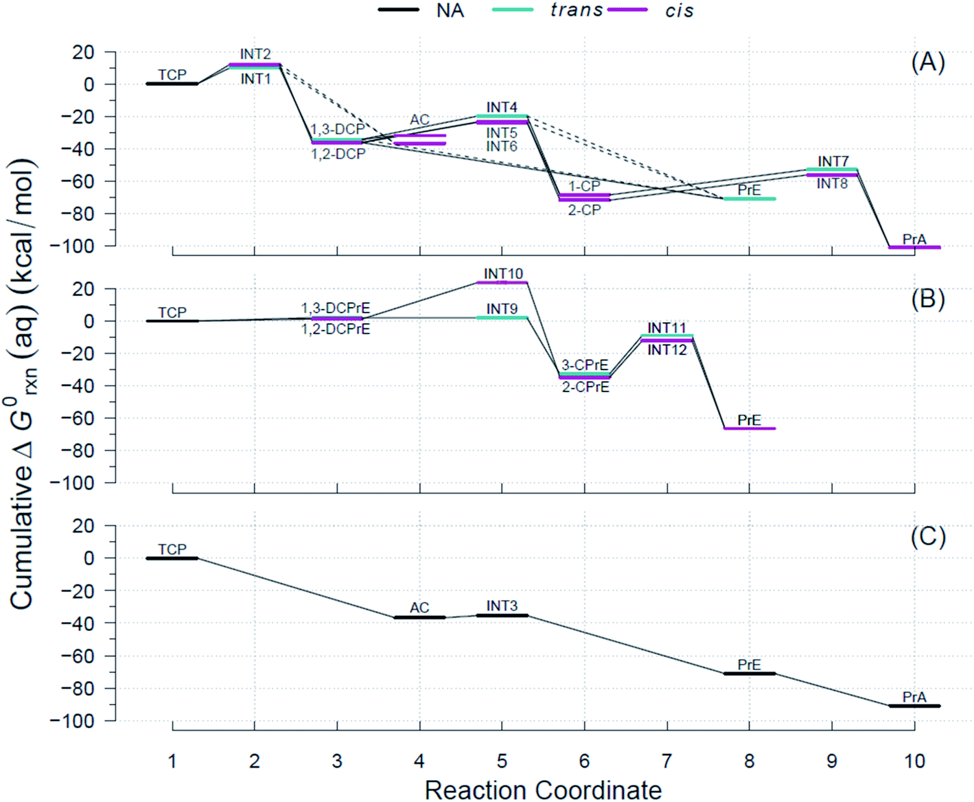 | ||
| Fig. 4 Example Reaction Coordinate Diagrams (RCDs) with energies computed using CCSD(T) for all the reactions shown in Fig. 2. RCDs using DFT methods in ESI (Fig. S2–S5†). (A) Pathway (1): HGL, (B) pathway (2): DHX, and (C) pathway (3): BRE + HDG. Reaction coordinate (RC): compound specific, assigned to main reaction products, and incremental with pathway progression (see RCDs sections for details). RCs and abbreviations listed and defined in Table S1.† Aqueous phase Gibbs free energies (ΔG0rxn(aq), kcal mol−1): cumulative at each RC yielding a pathway energy profile, i.e., a RCD. Colored lines at RC indicate relative molecular structure position of two Cl atoms. Dashed connecting lines indicate reactions of uncertain likelihood. H-atom model used: hydron (H+) (see Section 3.3 for details). | ||
The energy requirements for a particular reaction to proceed are indicated by the slope of the lines connecting the two corresponding RCs in Fig. 4, with smaller and/or negative slopes pointing to more energetically favorable reactions. Large drops in the RCDs, therefore, signal reactions that are more favorable thermodynamically. The reactions that have an intermediate (INT#) as a product are the only ones that result in ascending slopes, because the energies of the radicals are at a higher level than those of their preceding ground states. Comparison of the RCDs among the three main pathways considered shows that the BRE + HDG pathway (panel (C) in Fig. 4) is the only one with shallow slopes for intermediate species (AC → INT3 in Fig. 4(C)), while the other pathways demand significantly higher ΔG0rxn(aq) values for reactions involving radical species.
The energy profiles shown in Fig. 4 suggest that the BRE + HDG pathway (panel (C)) is more thermodynamically favorable for the transformation of TCP than either HGL (panel (A)) or DHX (panel (B)). This is due to two contributing factors, (i) deep descents in all RCs involving ground state species and (ii) absence of large positive slopes at any RC. The BRE + HDG pathway has a sharp decrease (∼37 kcal mol−1 units) for the first RC (i.e., Rxn # 7 to AC) while DHX results in positive slopes (from an increase of 1 to 2 kcal mol−1) for its corresponding first stable products (i.e., DCPrE isomers) making the latter pathway comparatively very energetically unfavorable.
Relative to the HGL pathway, the BRE + HDG has less intermediate species (only INT3) in its route to the final product (PrA), in contrast to the three RC intermediates in HGL. The energy profile involving INT3 has a shallow positive slope (increase of 1 kcal mol−1) in comparison with the significant energy requirements (20 to 30 kcal mol−1 units) in the HGL for RCs involving radicals as products. Instead of compensating for these larger energy demands with large energy drops, and even without taking intermediate species into consideration, HGL results in only similar descents for the first completely dechlorinated product (i.e., Rxn # 18, DCP → PrE), common to all three pathways, relative to that in BRE + HDG (both ≈35 kcal mol−1 units).
These lower energy requirements for radical intermediates and higher energy drops for stable products throughout the transformation route, make BRE + HDG a more energetically favorable pathway than either HGL or DHX. The differences in energies between trans- and cis-isomer routes are very small in all pathways (≤3.6 kcal mol−1) as seen by the overlapping colored lines in Fig. 4, with the exception of INT9 and INT10 in the DHX pathway.
3.6. Validation against data
To provide preliminary validation of the modeling results described above, a limited number of batch experiments were performed using zerovalent zinc (ZVZ) as the reductant and methods similar to those described in previous work.9,27 ZVZ is a very strong reductant thermodynamically (−0.76 V vs. SHE; cf. −0.44 for Fe0 (ref. 85)), although rates of reduction by ZVZ vary greatly with conditions at the metal surface (i.e., type and degree of passivation).27 ZVZ has been used for pilot- and field-scale remediation of TCP contaminated groundwater,15,26 but its utility in this study also stems from its potential to drive any of the possible reaction types in Fig. 1. In contrast, the available experimental data for TCP reduction by zerovalent iron (ZVI) suggests that system would give very limited reaction of TCP under most batch experimental conditions.9,28,29Batch experiments were performed by measuring the concentration of parent compound and products, starting with TCP or one of the three intermediates shown in Fig. 2: 1,2-dichloropropane, 1,3-dichloropropane, and allyl chloride. These intermediates were selected to constrain the kinetics of the thermodynamically favored reaction sequence determined from the modeling described above. Other possible intermediates, such as the chloropropenes shown in Fig. 2, were not investigated because they are not very favorable thermodynamically and no evidence for them had been seen in previous experimental work with ZVZ.9,27 The new data (Fig. S6†) show disappearance of each starting material is mainly accompanied by appearance of propene, with little or no detection of chlorinated intermediates. Mole balances calculated from parent compound disappearance and propene appearance were roughly 100% in all cases. Control experiments with the parent compound and without ZVZ showed negligable loss in all cases. The disappearance data fit well to a pseudo first-order model, as shown in Fig. S8.† The fitting coefficients are given as pseudo first-order rates constants (kobs) in Table 1, together with one standard deviations around the fit, which show that the kobs are reliable in all cases.
| Compound | k obs (h−1) | k SA (L g−1 m−2) |
|---|---|---|
| a k obs: pseudo first-order rate constant; kSA: first-order rate constant normalized to reactive surface area of reductant. | ||
| TCP | (1.36 ± 0.14) × 10−1 | (5.44 ± 0.56) × 10−4 |
| 1,2-DCP | (1.165 ± 0.078) × 10−2 | (4.66 ± 0.32) × 10−5 |
| 1,3-DCP | (8.1 ± 3.4) × 10−4 | (3.24 ± 1.4) × 10−6 |
| Allyl chloride | (7.29 ± 0.47) | (2.92 ± 0.19) × 10−2 |
When TCP was the starting material, the only chlorinated intermediate detected was allyl chloride, which was detected at trace concentrations only when the initial concentration of TCP was relatively high compared to previous work9,27 (Fig. S7†), suggesting allyl chloride is a short-lived intermediate. This is consistent with the data presented in Fig. S6 and S8† and summarized in Table 1, which show that the kobs for allyl chloride disappearance is an order of magnitude faster that the kobs for TCP disappearance under similar conditions. Conversely, the kobs for 1,2-dichloropropene and 1,3-dichloropropene disappearance are 1 and 3 orders-of-magnitude slower than the kobs for TCP appearance, respectively, suggesting that they would have accumulated within the batch reactor (and been detected) if they were formed to an appreciable degree. A sequential, pseudo first-order kinetic model for the reduction of TCP to allyl chloride to propene is described in the ESI (eqn (S2)–(S4)†) and was used to predict the kinetics of allyl chloride appearance/disappearance and propene appearance in experiments were TCP is the starting material. When the kinetic model was parameterized with the TCP and allyl chloride kobs presented in Table 1, it accurately predicted the experimental observations of allyl chloride appearance/disappearance and propene appearance in experiments were TCP was the starting material (Fig. S8†). This result further supports a reaction pathway in which TCP is reduced to allyl chloride through BRE followed by HGL to form propene without significant formation of other intermediates. This is consistent with the computed reaction coordinate analysis (e.g., Fig. 4), which suggest BRE of TCP is the most favorable reduction pathway.
4. Conclusions
The even distribution of chlorines along a propane backbone makes TCP a potential model for the degradation of other LHHCs. Under anaerobic conditions, TCP can undergo a combination of reduction, substitution, and elimination reactions that creates a network of reaction steps with intermediates that involves related LHHCs of environmental interest. These intermediates include other chlorinated propanes (e.g., 1,2-DCP) and propenes (e.g., 1,3-DCPrE) that are found in soil fumigant formulations, industrial feedstocks for polymers, etc.3 The theoretical and experimental results reported here show that hydrogenolysis is unfavorable to start, but if β-reductive elimination forms allyl chloride, then further hydrogenolysis of the remaining chlorine is rapid. The combination of steps results in complete dechlorination without the accumulation of persistant halogenated byproducts such as the dichloroethenes from trichloroethylene or chloroform from carbon tetrachloride. Other contaminants with analogous chemical structures to TCP range from 1,2-dichloroethane (1,2-DCA)32,86 to hexachlorocyclohexane (HCH, including lindane),87,88 so further analysis of their environmental fate might benefit from application of the computational methods and analysis developed here for TCP.Conflicts of interest
There are no conflicts to declare.Acknowledgements
This work was supported by the Strategic Environmental Research and Development Program (SERDP), mainly through Project ER-1458, and secondarily by ER-2620 and -2621. The modeling portion of this research was performed using the Institutional Computing facility (PIC) at the Pacific Northwest National Laboratory (PNNL) and the Chinook, Barracuda, and Cascade computing resources at the Environmental Molecular Sciences Laboratory (EMSL). PNNL is operated by Battelle Memorial Institute for the U.S. Department of Energy (DOE). EMSL is a National Scientific User Facility, located at PNNL, and sponsored by the DOE's Office of Biological and Environmental Research (DE-AC06-76RLO 1830). We also acknowledge EMSL for supporting the development of NWChem. This report has not been subject to review by any of the sponsors and therefore does not necessarily reflect their views and no official endorsement should be inferred.References
- California State Water Resources Control Board, Adopting the Proposed Regulations for a 1,2,3-Trichloropropane (1,2,3-TCP) maximum Contaminant Level (MCL) of 5 Parts Per Trillion, https://www.waterboards.ca.gov/drinking_water/certlic/drinkingwater/documents/123-tcp/sbddw17_001/tab12/rs2017_0042.pdf, 2017 Search PubMed.
- OEHHA, Public Health Goals for 1,2,3-Trichloropropane in Drinking Water, Office of Environmental Health and Hazard Assesment (OEHHA), California Environmental Protection Agency, 2009, https://www.waterboards.ca.gov/drinking_water/certlic/drinkingwater/documents/123-tcp/sbddw17_001/doc.pdf Search PubMed.
- K. R. Burow, W. D. Floyd and M. K. Landon, Factors affecting 1,2,3-trichloropropane contamination in groundwater in California, Sci. Total Environ., 2019, 672, 324–334, DOI:10.1016/j.scitotenv.2019.03.420.
- D. S. Oki and T. W. Giambelluca, DBCP, EDB, and TCP contamination of ground water in Hawaii, Ground Water, 1987, 25, 693–702, DOI:10.1111/j.1745-6584.1987.tb02210.x.
- E. P. Hooker, K. G. Fulcher and H. J. Gibb, Report to the Hawaii Department of Health, Safe Drinking Water Branch, Regarding the Human Health Risks of 1,2,3-Trichloropropane in Tap Water, Tetra Tech, Arlington, VA, 2012, https://eha-web.doh.hawaii.gov/eha-cma/documents/fd65a6d2-73d1-4d5c-88c6-97a47ba36650 Search PubMed.
- Hawaii Department of Health, Hawaii Administrative Rules, Title 11, Department of Health, Chapter 20, Rules Relating to Public Water Systems, 2018, https://health.hawaii.gov/opppd/files/2018/02/11-20.pdf Search PubMed.
- New Jersey Drinking Water Quality Institute, Maximum Contaminant Level Recommendations for 1,2,3-Trichloropropane in Drinking Water, Trenton, NJ, 2016, https://www.nj.gov/dep/watersupply/pdf/123-tcp-recommend.pdf Search PubMed.
- New Jersey Department of Environmental Protection, Drinking Water Standards by Constituent, 2018, https://www.nj.gov/dep/standards/drinking.water.pdf Search PubMed.
- V. Sarathy, P. G. Tratnyek, A. J. Salter, J. T. Nurmi, R. L. Johnson and G. O'Brien Johnson, Degradation of 1,2,3-trichloropropane (TCP): hydrolysis, elimination, and reduction by iron and zinc, Environ. Sci. Technol., 2010, 44, 787–793, DOI:10.1021/es902595j.
- G. Samin and D. B. Janssen, Transformation and biodegradation of 1,2,3-trichloropropane (TCP), Environ. Sci. Pollut. Res., 2012, 19, 3067–3078, DOI:10.1007/s11356-012-0859-3.
- R. W. Babcock, B. K. Harada, K. M. Lamichhane and K. T. Tsubota, Adsorption of 1,2,3-trichloropropane (TCP) to meet a MCL of 5 ppt, Environ. Pollut., 2018, 233, 910–915, DOI:10.1016/j.envpol.2017.09.085.
- California State Water Resources Control Board, 1,2,3-Trichloropropane (TCP), Division of Water Quality, GAMA Program, 2017, https://www.waterboards.ca.gov/gama/docs/coc_tcp123.pdf Search PubMed.
- K. Ozekin, 1,2,3-Trichloropropane State of the Science, Water Research Foundation, 2016, https://www.enviro.wiki/images/d/d2/1%2C2%2C3-Trichloropropane_state_of_science.pdf Search PubMed.
- V. L. Snoeyink and R. S. Summers, Adsorption of organic compounds, in Water Quality and Treatment: A Handbook of Community Water Supplies, ed. R. D. Letterman, American Water Works Association, 5th edn, 1999, ch. 13, pp. 13.11–13.83 Search PubMed.
- J. P. Merrill, E. J. Suchomel, S. Varadhan, M. Asher, L. Z. Kane, E. L. Hawley and R. A. Deeb, Development and validation of technologies for remediation of 1,2,3-trichloropropane in groundwater, Curr. Pollut. Rep., 2019, 5(4), 228–237, DOI:10.1007/s40726-019-00122-7.
- D. R. U. Knappe, R. S. Ingham, J. J. Moreno-Barbosa, M. Sun, R. S. Summers and T. Dougherty, Evaluation of Henry's Law Constants and Freundlich Adsorption Constants for VOCs, Water Research Foundation, Denver, CO, 2017, 4462_FinalReport_Published.pdf Search PubMed.
- C. H. Bell, M. Gentile, E. Kalve, I. Ross, J. Horst and S. Suthersan, Emerging Contaminants Handbook, CRC Press, 2019 Search PubMed.
- B. Wang and K.-H. Chu, Cometabolic biodegradation of 1,2,3-trichloropropane by propane-oxidizing bacteria, Chemosphere, 2017, 168, 1494–1497, DOI:10.1016/j.chemosphere.2016.12.007.
- M. Schmitt, S. Varadhan, S. Dworatzek, J. Webb and E. Suchomel, Optimization and validation of enhanced biological reduction of 1,2,3-trichloropropane in groundwater, Biorem. J., 2017, 28, 17–25, DOI:10.1002/rem.21539.
- J. Yan, B. A. Rash, F. A. Rainey and W. M. Moe, Isolation of novel bacteria within the Chloroflexi capable of reductive dechlorination of 1,2,3-trichloropropane, Environ. Microbiol., 2009, 11, 833–843, DOI:10.1111/j.1462-2920.2008.01804.x.
- K. Mukherjee, K. S. Bowman, F. A. Rainey, S. Siddaramappa, J. F. Challacombe and W. M. Moe, Dehalogenimonas lykanthroporepellens BL-DC-9T simultaneously transcribes many rdhA genes during organohalide respiration with 1,2-DCA, 1,2-DCP, and 1,2,3-TCP as electron acceptors, FEMS Microbiol. Lett., 2014, 354, 111–118, DOI:10.1111/1574-6968.12434.
- M. Lahoda, J. R. Mesters, A. Stsiapanava, R. Chaloupkova, M. Kuty, J. Damborsky and I. Kuta Smatanova, Crystallographic analysis of 1,2,3-trichloropropane biodegradation by the haloalkane dehalogenase DhaA31, Acta Crystallogr., Sect. D: Biol. Crystallogr., 2014, 70, 209–217, DOI:10.1107/s1399004713026254.
- M. Lahoda, R. Chaloupkova, A. Stsiapanava, J. Damborsky and S. I. Kuta, Crystallization and crystallographic analysis of the Rhodococcus rhodochrous NCIMB 13064 DhaA mutant DhaA31 and its complex with 1,2,3-trichloropropane, Acta Crystallogr., Sect. F: Struct. Biol. Cryst. Commun., 2011, 67, 397–400, DOI:10.1107/s1744309111001254.
- P. Dvorak, S. Bidmanova, J. Damborsky and Z. Prokop, Immobilized synthetic pathway for biodegradation of toxic recalcitrant pollutant 1,2,3-trichloropropane, Environ. Sci. Technol., 2014, 48, 6859–6866, DOI:10.1021/es500396r.
- T. Bosma, J. Damborsky, G. Stucki and D. B. Janssen, Biodegradation of 1,2,3-trichloropropane through directed evolution and heterologous expression of a haloalkane dehalogenase gene, Appl. Environ. Microbiol., 2002, 68, 3582–3587, DOI:10.1128/aem.68.7.3582-3587.2002.
- A. J. Salter-Blanc, E. J. Suchomel, J. H. Fortuna, J. T. Nurmi, C. Walker, T. Krug, S. O'Hara, N. Ruiz, T. Morley and P. G. Tratnyek, Evaluation of zerovalent zinc for treatment of 1,2,3-trichloropropane contaminated groundwater: laboratory and field assessment, Groundwater Monit. Rem., 2012, 32, 42–52, DOI:10.1111/j.1745-6592.2012.01402.x.
- A. J. Salter-Blanc and P. G. Tratnyek, Effects of solution chemistry on the dechlorination of 1,2,3-trichloropropane by zero-valent zinc, Environ. Sci. Technol., 2011, 45, 4073–4079, DOI:10.1021/es104081p.
- H. Li, Z.-T. Han, C.-X. Ma and J.-Y. Gui, Comparison of 1,2,3-trichloropropane reduction and oxidation by nanoscale zero-valent iron, zinc and activated persulfate, J. Groundw. Sci. Eng., 2015, 3, 156–163 Search PubMed.
- N. Lapeyrouse, M. Liu, S. Zou, G. Booth and C. L. Yestrebsky, Remediation of chlorinated alkanes by vitamin B12 and zero-valent iron, J. Chem., 2019, 2019, 8, DOI:10.1155/2019/7565464.
- H. Li, Z. Han, Y. Qian, X. Kong and P. Wang, In situ persulfate oxidation of 1,2,3-trichloropropane in groundwater of North China Plain, Int. J. Environ. Res. Public Health, 2019, 16, 2752, DOI:10.3390/ijerph16152752.
- C. G. Coyle, S. A. Waisner, V. F. Medina and C. S. Griggs, Use of dilute ammonia gas for treatment of 1,2,3-trichloropropane and explosives-contaminated soils, J. Environ. Manage., 2017, 204, 775–782, DOI:10.1016/j.jenvman.2017.03.098.
- P. Peng, U. Schneidewind, P. J. Haest, T. N. P. Bosma, A. S. Danko, H. Smidt and S. Atashgahi, Reductive dechlorination of 1,2-dichloroethane in the presence of chloroethenes and 1,2-dichloropropane as co-contaminants, Appl. Microbiol. Biotechnol., 2019, 103, 6837–6849, DOI:10.1007/s00253-019-09985-8.
- A. D. Maness, K. S. Bowman, J. Yan, F. A. Rainey and W. M. Moe, Dehalogenimonas spp. can reductively dehalogenate high concentrations of 1,2-dichloroethane, 1,2-dichloropropane and 1,1,2-trichloroethane, AMB Express, 2012, 2(54), 57, DOI:10.1186/2191-0855-2-54.
- A. L. Roberts, P. M. Jeffers, N. L. Wolfe and P. M. Gschwend, Structure-reactivity relationships in dehydrohalogenation reactions of polychlorinated and polybrominated alkanes, Crit. Rev. Environ. Sci. Technol., 1993, 23, 1–39, DOI:10.1080/10643389309388440.
- R. A. Larson and E. J. Weber, Reaction Mechanisms in Environmental Organic Chemistry, Lewis, Chelsea, MI, 1994 Search PubMed.
- M. Elsner and T. B. Hofstetter, Current perspectives on the mechanisms of chlorohydrocarbon degradation in subsurface environments: insight from kinetics, product formation, probe molecules and isotope fractionation, in Aquatic Redox Chemistry, ed. P. G. Tratnyek, T. J. Grundl and S. B. Haderlein, American Chemical Society, Washington, DC, 2011, vol. 1071, ch. 19, pp. 407–439, DOI:10.1021/bk-2011-1071.ch019.
- C. E. Schaefer, P. Ho, E. Berns and C. Werth, Mechanisms for abiotic dechlorination of trichloroethene by ferrous minerals under oxic and anoxic conditions in natural sediments, Environ. Sci. Technol., 2018, 52, 13747–13755, DOI:10.1021/acs.est.8b04108.
- X. Liu, S. Yuan, M. Tong and D. Liu, Oxidation of trichloroethylene by the hydroxyl radicals produced from oxygenation of reduced nontronite, Water Res., 2017, 113, 72–79, DOI:10.1016/j.watres.2017.02.012.
- H. T. Pham, M. Kitsuneduka, J. Hara, K. Suto and C. Inoue, Trichloroethylene transformation by natural mineral pyrite: the deciding role of oxygen, Environ. Sci. Technol., 2008, 42, 7470–7475, DOI:10.1021/es801310y.
- P. G. Tratnyek, E. Bylaska and E. J. Weber, In silico environmental chemical science: properties and processes from statistical and computational modelling, Environ. Sci.: Processes Impacts, 2017, 19, 188–202, 10.1039/c7em00053g.
- E. J. Bylaska, Estimating the thermodynamics and kinetics of chlorinated hydrocarbon degradation, Theor. Chem. Acc., 2006, 116, 281–296, DOI:10.1007/s00214-005-0042-8.
- L. Sviatenko, O. Isayev, L. Gorb, F. Hill and J. Leszczynski, Toward robust computational electrochemical predicting the environmental fate of organic pollutants, J. Comput. Chem., 2011, 32, 2195–2203, DOI:10.1002/jcc.21803.
- N. Sizochenko, D. Majumdar, S. Roszak and J. Leszczynski, Application of quantum mechanics and molecular mechanics in chemoinformatics, in Handbook of Computational Chemistry, ed. J. Leszczynski, Springer Netherlands, Dordrecht, 2016, pp. 1–23, DOI:10.1007/978-94-007-6169-8_52-1.
- C. J. Cramer, Essentials of Computational Chemistry: Theories and Models, Wiley, Chichester, 2nd edn, 2013 Search PubMed.
- E. J. Bylaska, K. R. Glaesemann, A. R. Felmy, M. Vasiliu, D. A. Dixon and P. G. Tratnyek, Free energies for degradation reactions of 1,2,3-trichloropropane from ab initio electronic structure theory, J. Phys. Chem. A, 2010, 114, 12269–12282, DOI:10.1021/jp105726u.
- A. J. Salter-Blanc, E. J. Bylaska, M. A. Lyon, S. Ness and P. G. Tratnyek, Structure-activity relationships for rates of aromatic amine oxidation by manganese dioxide, Environ. Sci. Technol., 2016, 50, 5094–5102, DOI:10.1021/acs.est.6b00924.
- A. S. Pavitt, E. J. Bylaska and P. G. Tratnyek, Oxidation potentials of phenols and anilines: correlation analysis of electrochemical and theoretical values, Environ. Sci.: Processes Impacts, 2017, 19, 339–349, 10.1039/c6em00694a.
- M. Valiev, E. J. Bylaska, N. Govind, K. Kowalski, T. P. Straatsma, H. J. J. Van Dam, D. Wang, J. Nieplocha, E. Apra, T. L. Windus and W. A. de Jong, NWChem: a comprehensive and scalable open-source solution for large scale molecular simulations, Comput. Phys. Commun., 2010, 181, 1477–1489, DOI:10.1016/j.cpc.2010.04.018.
- E. J. Bylaska, EMSL Arrows, https://arrows.emsl.pnnl.gov/api/ Search PubMed.
- W. Kohn and L. J. Sham, Self-consistent equations including exchange and correlation effects, Phys. Rev., 1965, 140, 1133–1138, DOI:10.1103/physrev.140.a1133.
- R. G. Parr, Density functional theory of atoms and molecules, in Horizons of Quantum Chemistry, Springer, 1980, pp. 5–15 Search PubMed.
- S. Ghosh, P. Verma, C. J. Cramer, L. Gagliardi and D. G. Truhlar, Combining wave function methods with density functional theory for excited states, Chem. Rev., 2018, 118, 7249–7292, DOI:10.1021/acs.chemrev.8b00193.
- R. J. Bartlett and J. F. Stanton, Applications of post-Hartree—Fock methods: a tutorial, in Reviews in Computational Chemistry, ed. K. B. Lipkowitz and D. B. Boyd, Wiley, 1994, vol. 5, pp. 65–169, DOI:10.1002/9780470125823.ch2.
- R. J. Bartlett and M. Musiał, Coupled-cluster theory in quantum chemistry, Rev. Mod. Phys., 2007, 79, 291 CrossRef CAS.
- E. V. Patterson, C. J. Cramer and D. G. Truhlar, Reductive dechlorination of hexachloroethane in the environment: mechanistic studies via computational electrochemistry, J. Am. Chem. Soc., 2001, 123, 2025–2031, DOI:10.1021/ja0035349.
- S. Pari, I. Wang, H. Liu and B. Wong, Sulfate radical oxidation of aromatic contaminants: a detailed assessment of density functional theory and high-level quantum chemical methods, Environ. Sci.: Processes Impacts, 2017, 19, 395–404, 10.1039/c7em00009j.
- R. Krishnan, J. S. Binkley, R. Seeger and J. A. Pople, Self-consistent molecular orbital methods. XX. A basis set for correlated wave functions, J. Chem. Phys., 1980, 72, 650–654, DOI:10.1063/1.438955.
- A. D. Becke, Density-functional thermochemistry. III. The role of exact exchange, J. Chem. Phys., 1993, 98, 5648–5652, DOI:10.1063/1.464913.
- J. F. Stanton, Why CCSD (T) works: a different perspective, Chem. Phys. Lett., 1997, 281, 130–134, DOI:10.1016/S0009-2614(97)01144-5.
- A. G. Taube and R. J. Bartlett, Improving upon CCSD (T): Λ CCSD (T). I. Potential energy surfaces, J. Chem. Phys., 2008, 128, 044110, DOI:10.1063/1.2830236.
- T. Clark, J. Chandrasekhar, G. W. Spitznagel and P. v. R. Schleyer, Efficient diffuse function-augmented basis sets for anion calculations. III. The 3-21+G basis set for first-row elements, Li to F., J. Comput. Chem., 1983, 4, 294–301, DOI:10.1002/jcc.540040303.
- C. Lee, W. Yang and R. G. Parr, Development of the Colle-Salvetti correlation-energy formula into a functional of electron density, Phys. Rev. B: Condens. Matter Mater. Phys., 1988, 37, 785–789 CrossRef CAS PubMed.
- C. Adamo and V. Barone, Toward reliable density functional methods without adjustable parameters: the PBE0 model, J. Chem. Phys., 1999, 110, 6158 CrossRef CAS.
- J. P. Perdew, K. Burke and M. Ernzerhof, Generalized gradient approximation made simple, Phys. Rev. Lett., 1996, 77, 3865 CrossRef CAS PubMed.
- Y. Zhao and D. G. Truhlar, The M06 suite of density functionals for main group thermochemistry, thermochemical kinetics, noncovalent interactions, excited states, and transition elements: two new functionals and systematic testing of four M06-class functionals and 12 other functionals, Theor. Chem. Acc., 2008, 120, 215–241 Search PubMed.
- A. Klamt and G. Schüürmann, COSMO: a new approach to dielectric screening in solvents with explicit expressions for the screening energy and its gradient, J. Chem. Soc., Perkin Trans. 2, 1993, 799–803 RSC.
- D. H. Evans, Solution electron-transfer reactions in organic and organometallic electrochemistry, Chem. Rev., 1990, 90, 739–751 CrossRef CAS.
- L. A. Totten, U. Jans and A. L. Roberts, Alkyl bromides as mechanistic probes of reductive dehalogenation: reactions of vicinal dibromide stereoisomers with zerovalent metals, Environ. Sci. Technol., 2001, 35, 2268–2274, DOI:10.1021/es0010195.
- O. Isayev, L. Gorb and J. Leszczynski, Theoretical calculations: can Gibbs free energy for intermolecular complexes be predicted efficiently and accurately?, J. Comput. Chem., 2007, 28, 1598–1609, DOI:10.1002/jcc.20696.
- M. Li, X. Yang and Y. Xue, Comparison of DFT, MP2/CBS, and CCSD(T)/CBS methods for a dual-level QM/MM Monte Carlo simulation approach calculating the free energy of activation of reactions in solution and “on water”: a case study, Theor. Chem. Acc., 2017, 136, 69, DOI:10.1007/s00214-017-2103-1.
- N. Mardirossian and M. Head-Gordon, Thirty years of density functional theory in computational chemistry: an overview and extensive assessment of 200 density functionals, Mol. Phys., 2017, 115, 2315–2372, DOI:10.1080/00268976.2017.1333644.
- L. Goerigk and N. Mehta, A trip to the density functional theory zoo: warnings and recommendations for the user, Aust. J. Chem., 2019, 72, 563–573 CrossRef CAS.
- D. Lee and K. Burke, Finding electron affinities with approximate density functionals, Mol. Phys., 2010, 108, 2687–2701, DOI:10.1080/00268976.2010.521776.
- M. Lingwood, J. R. Hammond, D. A. Hrovat, J. M. Mayer and W. T. Borden, MPW1K performs much better than B3LYP in DFT calculations on reactions that proceed by proton-coupled electron transfer (PCET), J. Chem. Theory Comput., 2006, 2, 740–745, DOI:10.1021/ct050282z.
- G. Bistoni, Finding chemical concepts in the Hilbert space: coupled cluster analyses of noncovalent interactions, Wiley Interdisciplinary Reviews: Computational Molecular Science, 2019, p. e1442, DOI:10.1002/wcms.1442.
- C. Suellen, R. G. Freitas, P.-F. Loos and D. Jacquemin, Cross-comparisons between experiment, TD-DFT, CC, and ADC for transition energies, J. Chem. Theory Comput., 2019, 15, 4581–4590, DOI:10.1021/acs.jctc.9b00446.
- Y. He, Z. He and D. Cremer, Comparison of CCSDT-n methods with coupled-cluster theory with single and double excitations and coupled-cluster theory with single, double, and triple excitations in terms of many-body perturbation theory – what is the most effective triple-excitation method?, Theor. Chem. Acc., 2001, 105, 182–196, DOI:10.1007/s002140000196.
- I. Y. Zhang and A. Grüneis, Coupled cluster theory in materials science, Front. Mater., 2019, 6 DOI:10.3389/fmats.2019.00123.
- D. G. Liakos and F. Neese, Is it possible to obtain coupled cluster quality energies at near density functional theory cost? Domain-based local pair natural orbital coupled cluster vs. modern density functional theory, J. Chem. Theory Comput., 2015, 11, 4054–4063, DOI:10.1021/acs.jctc.5b00359.
- M. D. Tissandier, K. A. Cowen, W. Y. Feng, E. Gundlach, M. H. Cohen, A. D. Earhart, J. V. Coe and T. R. Tuttle, The proton's absolute aqueous enthalpy and Gibbs free energy of solvation from cluster-ion solvation data, J. Phys. Chem. A, 1998, 102, 7787–7794, DOI:10.1021/jp982638r.
- L. K. Sviatenko, L. Gorb, D. Leszczynska, S. I. Okovytyy, M. K. Shukla and J. Leszczynski, Role of singlet oxygen in the degradation of selected insensitive munitions compounds: a comprehensive, quantum chemical investigation, J. Phys. Chem. A, 2019, 123, 7597–7608, DOI:10.1021/acs.jpca.9b01772.
- M. Yasir Kahn, S. So and G. da Silva, Decomposition kinetics of perfluorinated sulfonic acids, Chemosphere, 2019, 238, 124615, DOI:10.1016/j.chemosphere.2019.124615.
- R. Development Core Team, R: A language and environment for statistical computing, R Foundation for Statistical Computing, Vienna, Austria, 3.2.0 edn., 2015 Search PubMed.
- T. L. Torralba-Sanchez and P. G. Tratnyek, R script for the automated generation of reaction coordinate diagrams (RCDs) of chemical reaction energies and transformation networks, Zenodo, 25 January 2020, DOI:10.5281/zenodo.3611472.
- M. Pourbaix, Atlas of Electrochemical Equilibria in Aqueous Solutions, National Association of Corrosion Engineers, Houston, TX, 1974 Search PubMed.
- A. Nunez Garcia, H. K. Boparai and D. M. O'Carroll, Enhanced dechlorination of 1,2-dichloroethane by coupled nano iron-dithionite treatment, Environ. Sci. Technol., 2016, 50, 5243–5251, DOI:10.1021/acs.est.6b00734.
- N. Zhang, S. Bashir, J. Qin, J. Schindelka, A. Fischer, I. Nijenhuis, H. Herrmann, L. Y. Wick and H. H. Richnow, Compound specific stable isotope analysis (CSIA) to characterize transformation mechanisms of α-hexachlorocyclohexane, J. Hazard. Mater., 2014, 280, 750–757, DOI:10.1016/j.jhazmat.2014.08.046.
- S. Wacławek, D. Silvestri, P. Hrabák, V. V. T. Padil, R. Torres-Mendieta, M. Wacławek, M. Černík and D. D. Dionysiou, Chemical oxidation and reduction of hexachlorocyclohexanes: a review, Water Res., 2019, 162, 302–319, DOI:10.1016/j.watres.2019.06.072.
Footnote |
| † Electronic supplementary information (ESI) available. See DOI: 10.1039/c9em00557a |
| This journal is © The Royal Society of Chemistry 2020 |