
Discrimination and geo-spatial mapping of atmospheric VOC sources using full scan direct mass spectral data collected from a moving vehicle†
L. C.
Richards
 ab,
N. G.
Davey
a,
C. G.
Gill
abcd and
E. T.
Krogh
*ab
ab,
N. G.
Davey
a,
C. G.
Gill
abcd and
E. T.
Krogh
*ab
aApplied Environmental Research Laboratories, Chemistry Department, Vancouver Island University, Nanaimo, British Columbia, Canada. E-mail: Erik.Krogh@viu.ca
bDepartment of Chemistry, University of Victoria, Victoria, British Columbia, Canada
cChemistry Department, Simon Fraser University, Burnaby, B.C., Canada
dDepartment of Environmental and Occupational Health Sciences, University of Washington, Seattle, WA, USA
First published on 29th November 2019
Abstract
Volatile and semi-volatile organic compounds (S/VOCs) are ubiquitous in the environment, come from a wide variety of anthropogenic and biogenic sources, and are important determinants of environmental and human health due to their impacts on air quality. They can be continuously measured by direct mass spectrometry techniques without chromatographic separation by membrane introduction mass spectrometry (MIMS) and proton-transfer reaction time-of-flight mass spectrometry (PTR-ToF-MS). We report the operation of these instruments in a moving vehicle, producing full scan mass spectral data to fingerprint ambient S/VOC mixtures with high temporal and spatial resolution. We describe two field campaigns in which chemometric techniques are applied to the full scan MIMS and PTR-ToF-MS data collected with a mobile mass spectrometry lab. Principal Component Analysis (PCA) has been successfully employed in a supervised analysis to discriminate VOC samples collected near known VOC sources including internal combustion engines, sawmill operations, composting facilities, and pulp mills. A Gaussian mixture model and a density-based spatial clustering of application with noise (DBSCAN) algorithm have been used to identify sample clusters within the full time series dataset collected and we present geospatial maps to visualize the distribution of VOC sources measured by PTR-ToF-MS.
Environmental significanceVolatile organic compounds (VOCs) are emitted from anthropogenic and biogenic sources and are present at trace levels in the atmosphere. They contribute to degraded air quality as precursors to ground level ozone and secondary organic aerosol formation. In addition, some VOCs are toxic and some are associated with nuisance odours. We describe direct mass spectrometry continuously operated in a moving vehicle to capture changes in VOC composition over time and space. Principal component analysis was employed to discriminate sources with the results visualized to map sources, distributions, and potential impacts. This work has applications to neighbourhood scale air quality mapping, and can be generalized to other sensor data. It is an important first step in real-time source tracking and apportionment. |
Introduction
Volatile and semi-volatile organic compounds (S/VOCs) are important determinants of both environmental1,2 and human health.3 In the atmosphere, they are precursors in the formation of ground-level ozone,4 contribute to particulate matter through the formation of secondary organic aerosols,5 and can also have direct health effects (e.g., benzene is carcinogenic).3,6 Atmospheric S/VOCs have numerous point and diffuse sources, with both anthropogenic and biogenic origins.7 Their distributions can vary widely over time and space depending on proximity to sources, meteorological conditions, topography, and atmospheric chemical processes.7 Traditional methods of atmospheric VOC sampling involve the collection of samples in evacuated cannisters8 or onto sorbent tubes9,10 which are subsequently measured in a laboratory setting by gas chromatography mass spectrometry (GC-MS) or related techniques.8 While these methods allow for comprehensive VOC analysis, they are time consuming and labour intensive, and provide data for one fixed location and sampling time or period. As such, these lab-based methods do not capture fine scale variations in VOC concentrations over time and/or space. More recently, mass spectrometers have been installed at strategic stationary monitoring sites for VOC analysis, using continuous direct mass spectrometry, typically proton-transfer reaction mass spectrometry,11–15 and fast GC-detector systems.16–18 The resulting datasets can be used to identify VOC sources by examining temporal trends in individual compounds, such as the differing diurnal emission patterns for biogenic VOCs and aromatic hydrocarbons,13 and by applying receptor models to the full suite of measured compounds.12More recently, the miniaturization and ruggedization of analytical instrumentation has facilitated their use in moving vehicles, allowing for geospatial chemical mapping. In particular, the miniaturization of direct mass spectrometry instrumentation allows for continuous, on-road,19–23 underwater,24,25 and airborne15,26,27 measurements to map spatial and temporal distributions of S/VOC concentrations. Further, techniques such as proton-transfer reaction time-of-flight mass spectrometry (PTR-ToF-MS) and membrane introduction mass spectrometry (MIMS) allow for the simultaneous analysis of the mixture of S/VOCs in an air sample without chromatographic separation.28
MIMS employs a semipermeable membrane as an interface between the sample and the mass spectrometer.29–31 Air samples are continuously passed over a polydimethylsiloxane membrane and S/VOCs pervaporate into a carrier gas, where they are transferred to the mass spectrometer as a mixture for analysis. Electron ionization (EI) typically employed by these systems results in the initial formation of [M+˙] ions and subsequent fragmentation. MIMS is well suited for the analysis of small, hydrophobic molecules present in an air sample. The resulting full scan mass spectra represent the superposition of all of the ions produced by the mixture of VOCs permeating the membrane.19
In PTR-ToF-MS analysis, VOCs in a continuously sampled air stream are reacted with H3O+ reagent ions in a drift tube with a uniform electric field, where ion-molecule collisions occur. If the proton affinity (PA) of the analyte (M) is higher than that of water, protonated molecular ions [MH+] are formed. PTR is a softer ionization method than EI resulting in considerably less fragmentation.32 PTR-ToF-MS is an excellent method for directly analyzing both polar and non-polar trace organic compounds in ambient air without chromatographic separation.15,33 When coupled with time-of-flight mass spectrometry, full scan mass spectra are obtained in microseconds.
Both MIMS and PTR-ToF-MS systems have been operated on a mobile platform for temporally and spatially resolved quantitative analysis of ambient VOCs in the parts-per-trillion by volume (pptv) to parts-per-billion by volume (ppbv) range. PTR-ToF-MS systems have been operated on aircraft campaigns to measure and quantify VOCs in an agricultural fire plume and urban environments,26 as well as over oil and gas producing regions,34 and have been used ‘on-road’ to measure emissions from vehicles.23 Several researchers have employed PTR with quadrupole mass spectrometers to assess BVOC emissions above forested areas.35 Portable MIMS systems have been operated from a moving vehicle for quantitative VOC analysis near oil and gas activites,19,20 to detect products and impurities from methamphetamine precursor production,21 and to measure VOCs associated with traffic and woodsmoke emissions.22 These field studies focused on the identification and quantitation of individual VOCs or isomer classes by analyzing the signal intensity at specific mass-to-charge ratios (m/z) or by using targeted methods, such as tandem mass spectrometry (MS/MS) and/or selected ion monitoring (SIM) scans. Alternatively, qualitative chemometric analysis taking advantage of the wealth of non-targeted information present in a full scan mass spectrum can be used to discriminate between samples containing different VOC mixtures, but has not yet been applied to data collected on a mobile platform.28
Principal component analysis (PCA) is a multivariate dimensional reduction technique that calculates new variables, Principal Components (PCs), that are linear combinations of the original variables (m/z), as shown in eqn (1):
| PC = a1m/z1 + a2m/z2 + … + anm/zn | (1) |
PCA has been applied to data collected from MIMS and PTR-MS systems for sample discrimination in environmental28,38–41 and food39,42–44 analysis. Alberici et al. analyzed the full scan MIMS spectra of the water soluble fraction of Brazilian commercial gasolines using PCA,41 and Ketola et al. have used a similar approach to distinguish commercial drink products based on the manufacturer.42 PCA has also been employed to differentiate and classify terpene photo-oxidation mechanisms in atmospheric simulation chambers using data collected with a PTR-ToF-MS system.38 We have recently employed full scan MIMS data to discriminate lab-based constructed air samples, VOCs produced in the combustion of different species of wood, and headspace samples influenced by aqueous hydrocarbon solutions.28 None of these studies have exploited the high temporal resolution capabilities of direct mass spectrometry in a moving vehicle to provide geospatial maps of air masses influenced by different VOC sources.
Here we present MIMS and PTR-ToF-MS data collected on-road in a mobile mass spectrometry laboratory during field campaigns on central Vancouver Island, British Columbia (BC), Canada. We use PCA to analyze the full scan mass spectra to discriminate VOC sources in ambient air samples impacted by a variety of activities including vehicle exhaust, pulp mills, sawmills, and composting facilities. We describe a supervised approach, where selected data from the field campaigns was analyzed based on known nearby point sources, as well as an unsupervised approach, where the entire data set was analyzed using PCA followed by a Gaussian mixture model and density-based spatial clustering of application with noise (DBSCAN) algorithm in order to identify clusters within the data set. Both approaches allow for the discrimination of real-world VOC sources and can be used in combination with spatial information to generate neighborhood-scale maps illustrating the distribution of sources.
Experimental
The data presented here was collected during field campaigns on eastern Vancouver Island, BC, Canada in August 2016 (4 days) and August 2017 (2 days), using instruments mounted in a research purposed cargo van (4 × 4 2500 Cargo 144 Sprinter, Mercedes-Benz, Nanaimo, BC, Canada). The study area includes residential, commercial, industrial, and rural/light agricultural uses. The surrounding area is dominated by mixed coniferous forest, and marine environments. Field notes identified suspected stationary VOC point sources (e.g., gas stations, industrial sites, composting facilities) as well as mobile VOC sources (e.g., vehicle exhaust, transport trucks) encountered while driving. It should be noted that it was not always possible to identify a single VOC source as some sources are co-located and the ambient air was influenced by more than one source. Details from the field campaigns are described below and in ESI.†Membrane introduction mass spectrometry
A modified Griffin 400 EI (70 eV) with a cylindrical quadruple ion trap (CIT) mass spectrometer (FLIR, West Lafayette, IN, USA) described previously was used for the MIMS analysis.19 A 10 cm long polydimethylsiloxane (PDMS) capillary hollow fibre membrane (Silastic® brand; DowCorning, Midland, MI, USA) with 0.47 mm outer radius and 0.26 mm inner radius was employed, heated to 50 °C, with 1 mL min−1 of helium carrier gas (99.999% purity, Air Liquide, Nanaimo, BC, Canada) continuously passing through the membrane's lumen. The mass spectrometer was operated with a base pressure of 5 × 10⁻⁵ Torr, with the ion trap at 150 °C, using a maximum ionization time of 150 ms for full scan data collection. The MIMS instrument was encased in 0.1 mm thick mu-metal (μ ≈ 50![[thin space (1/6-em)]](https://www.rsc.org/images/entities/char_2009.gif) 000, McMaster Carr, Elmhurst, IL, USA) in order to reduce the effect of the Earth's magnetic field on the measured signal intensity.45 The MIMS instrument described has low ppbv sensitivity for hydrocarbons such as the BTEX suite (benzene, toluene, ethylbenzene, xylenes) and a compound dependent response time of 15–30 seconds due to membrane transport.
000, McMaster Carr, Elmhurst, IL, USA) in order to reduce the effect of the Earth's magnetic field on the measured signal intensity.45 The MIMS instrument described has low ppbv sensitivity for hydrocarbons such as the BTEX suite (benzene, toluene, ethylbenzene, xylenes) and a compound dependent response time of 15–30 seconds due to membrane transport.
The MIMS system was operated from an independent 24 VDC power supply (4 × 6 VDC lead acid batteries, Model S6-275AGM, Surrette Battery Company Ltd, Springhill, NS, Canada) in the vehicle. Ambient air was continuously flowed over the membrane interface at 2 L min−1 using a 1/4 inch outer diameter and 3/16 inch inner diameter fluorinated ethylene propylene (FEP) sampling line (Cole-Parmer, Montreal, QC, Canada) that was passed through the passenger side window and attached to the front of the vehicle 40 cm above the windshield. Two in-line stainless steel frit filters at 15 and 5 μm (Swagelok, Solon, OH, USA) were used to remove particulate matter from the sampling stream.
Field data was collected with the MIMS instrument on August 4, 5, 9, and 10, 2016 in the Nanaimo area of Vancouver Island, BC, Canada. Meteorological data for this field campaign is found in the ESI and summarized in Table S1.† Full scan MIMS mass spectra were collected every 7 seconds on August 4, 9, and 10, and every 1 second on August 5. Air was sampled near fresh paving at two different locations (asphalt samples), vehicle exhaust samples were collected roadside as vehicles were unloading from a ferry, as well as from vehicles encountered when sampling, gasoline samples were collected at a gas station (fresh) and from a storage container (aged), and additional road works samples were collected in the vicinity of the paving activities.
In addition to collecting full scan mass spectra for non-targeted VOC fingerprinting, several targeted quantitative scans were also included for context. Details of the quantitative analysis are found in the ESI, with Table S2† detailing calibration information. Ambient VOC concentrations were generally observed to be in the low ppbv range, with less than 5% of the observations above our quantitation limits (typically 3–6 ppbv) as illustrated in the whisker plots shown in Fig. S1 (ESI†). Concentration excursions above these limits were associated with sampling in close proximity to known point sources with concentrations up to 18 ppbv for benzene, 91 ppbv for toluene, 88 ppbv for ethylbenzene, and 26 ppbv for α-pinene.
Proton-transfer reaction time-of-flight mass spectrometry
The proton-transfer reaction time-of-flight mass spectrometer (PTR-TOF1000, Ionicon Analytik Ges.m.b.H, Innsbruck, Austria) was attached to a vibration-damping mount, with six air cushion supports (Stabl-Level, SLM-1, McMaster Carr) pressurized to 50 PSI to dampen vibration while the vehicle was in motion. The PTR-ToF-MS was powered from a custom 4800 Ah lithium ion battery bank (Canadian Electric Vehicles, Parksville, CAN) and 2800 W AC/DC inverter/charger (Magnasine, MS2012 2800–12 V, Sensata Tech, St. Paul, MN, USA) that is continuously float charged from a dedicated 220 amp engine alternator. A perfluoroalkoxy (PFA) sample line (4 m long, OD 1/4′′, ID 3/16′′, Cole-Parmer, Montreal, QC, Canada) was mounted on an aluminum sampling arm extending 1 m above the roof at the front of the vehicle, with an in-line 1 um filter (Swagelok). The sampling line was not heated, and ambient temperatures ranged from 24–27 °C during sampling. H3O+ was used as the reagent ion, and the instrument was mass calibrated every 5 s during sampling using the signals at m/z 21.022, 29.999, and 59.049 (H318O+, NO+, C3H7O+). The instrument resolution was 1500–2000 at m/z 59. An E/N of 130 Td and drift pressure of 2.20 mbar was used during sampling. The pressure inside the ToF was 1.2 × 10⁻⁶ mbar. The air sampling flow rate was 250 sccm, with a mass spectrum collected every 1 s. The transit time between the sample inlet and the mass spectrometer was about 10 seconds. The instrument is sensitive to sub parts-per-billion levels.Field campaign data was collected on August 21 and 22, 2017 between Nanaimo and Crofton, BC. Winds were light (2–4 m s−1) on all sampling days. Additional meteorological data for this field campaign is found in the ESI and summarized in Table S3.† Samples were collected near two different pulp mills, two sawmills, a wood storage site, two composting facilities (commercial operator and a topsoil producer), a landfill, a gas station, an auto wrecking facility, and a ferry terminal. Some sources were sampled on both days (e.g., composting facility). Mass spectra were collected at 1 Hz using the PTR-ToF-MS system, and high resolution positional data was collected using a roof mounted antenna (Hemisphere A45, Scottsdale, AZ) and GPS receiver (Hemisphere R330, GNSS Receiver, Scottsdale, AZ, USA). While the focus of this work was on qualitative analysis, direct calibrations for benzene, toluene, ethylbenzene, dimethyl sulfide, and α-pinene were also performed using certified permeation tubes in a Dynacalibrator Gas Dilution System with concentrations ranging up to 150 ppbv. Details of this work is found in the ESI, with Table S4† detailing the calibration information. Observed VOC concentrations were generally below 1 ppbv, with elevated levels up to 150 ppbv of dimethyl sulfide (m/z 63.022) being measured in the vicinity of a pulp mill. BTEX concentrations up to 25 ppbv benzene (m/z 79.049), 50 ppbv toluene (m/z 93.061), and 60 ppbv ethylbenzene (m/z 107.076) were measured near an auto wrecking facility. Terpene concentrations up to 56 pbbv (as α-pinene, m/z 137.110) were measured near a wood chip truck and sawmills. Whisker plots for VOC concentrations over the sampling period are shown in Fig. S2 in the ESI.†
Data analysis
Post deployment, the data collected for each day of the field campaigns was combined into a single file for interrogation. Mass lists for the PTR-ToF-MS were made using the PTRViewer 3 software (Version 3.2.8 Ionicon). Mass calibration for each of the data files was verified in the software using 5 scan averaging and signals at m/z 21.022, 29.997, and 59.049. After mass calibration, the mass spectra in each data file were summed up and then used to identify all m/z peaks present in the data set. For overlapping peaks, the Gauss fit tool in the PTRViewer 3 software was used to calculate overlapping mass spectral peak areas. Peak areas were corrected to account for differences in ion transmission through the mass analyzer using the instrument's transmission curve. PTR-ToF-MS data was normalized to the reagent ion signal at m/z 21.022 (H318O+) to account for ionization differences. For each field campaign a time series signal chronogram of the total ion current (TIC) data (m/z 30–215 excluding the signal intensities of O2+, H3OH2O+, and H3OH218O+ for the PTR-ToF-MS data, m/z 50–250 for the MIMS data) was examined to identify periods with higher VOC concentrations. We noticed some carry-over in the PTR-ToF-MS data after sampling near a composting facility (particularly at m/z 61.029, associated with acetic acid). On both days, the compost samples were collected at the end of the run and data impacted by carry-over was removed from the analysis.Supervised data analysis
Data associated with high total VOC concentrations was cross checked with the field notes to identify potential VOC sources. If a source was identified, average mass spectra were calculated by averaging the measured signal intensities across a 10–15 s time window for subsequent use in PCA. Mass spectra were background subtracted using the mass spectrum of ambient clean air. A dataset for each field campaign was generated by creating a data matrix, where each row contained an average mass spectrum for an identified sample, with the columns for the data matrix containing the measured m/z. Each mass spectrum in the dataset was normalized to a unit vector in order to remove concentration effects as follows: | (2) |
![[x with combining circumflex]](https://www.rsc.org/images/entities/i_char_0078_0302.gif) is the full scan mass spectrum as a vector of unit length. Each column was mean-centered to give each variable (m/z) a mean of zero. PCA was applied to the normalized and mean centered datasets. Data analysis was done using Microsoft Excel (Microsoft Corporation, Redmond, WA, USA), MATLAB (Mathworks, Natick, NA, USA), MATLAB's Statistics and Machine Learning Toolbox, and the PLS_Toolbox (Eigenvector Research Inc, Manson, WA, USA).
is the full scan mass spectrum as a vector of unit length. Each column was mean-centered to give each variable (m/z) a mean of zero. PCA was applied to the normalized and mean centered datasets. Data analysis was done using Microsoft Excel (Microsoft Corporation, Redmond, WA, USA), MATLAB (Mathworks, Natick, NA, USA), MATLAB's Statistics and Machine Learning Toolbox, and the PLS_Toolbox (Eigenvector Research Inc, Manson, WA, USA).
Unsupervised data analysis
Unsupervised cluster analysis was conducted on a PCA model of the PTR-ToF-MS data set collected on August 21 and 22, 2017 using two algorithms: Gaussian mixture model (GMM) algorithm and a density-based spatial clustering of applications with noise (DBSCAN) algorithm. The GMM algorithm calculates clusters by assuming the data set is composed of a specified number of clusters with Gaussian distributions with unknown means and covariance matrices.46 DBSCAN identifies core points that have a certain number of neighbours within a given neighbourhood and extends the clusters outwards from these core points, resulting in clusters of high density data. The number of clusters does not need to be specified beforehand, and the clusters can have any shape.47 For the GMM algorithm, the model was run using a random initiation for 2–20 groups, with 100 replicates per number of clusters, and a maximum of 10000 algorithm iterations per replicate. Models were run with covariance matrices being shared among the groups, unshared among the groups, and with both full and diagonal covariance matrices using modified MATLAB code.48 Akaike information criterion (AIC), and Bayesian information criterion (BIC) values were calculated for each of the 19 clustering options. Additional AIC and BIC values were calculated for up to 40 groups using full, unshared covariance matrices. The results from these metrics were then compared to inform the number of groups within the dataset. The final number of groups used in the analysis was determined by producing geospatial maps with different colours used for each group. These maps were then interrogated, and compared with field notes to determine the optimum clustering model. For the DBSCAN algorithm, neighbourhood size and the number of neighbours needed to identify core points were varied until the algorithm would identify multiple clusters within the PCA model. Once again, the final number of clusters was determined using a combination of geospatial maps and field notes.
Geospatial maps
Geospatial maps of the August 2017 field campaign were generated to visualize the spatial distribution of VOC sources in Google Earth (Google Earth, Google LLC, Mountain View, CA, USA) by using MATLAB to produce keyhole markup language (kml) files. The Komoot Outdoor Google Earth overlay was used to aid data visualization.49 Data was collected at a frequency of 1 Hz resulting in a spatial resolution of 15–25 m with drive speeds between 50 and 100 km per hour. As the GPS data and mass spectral data were not collected at the exact same timestamps, a location for each mass spectrum was determined by using a linear interpolation between the two latitude and longitude measurements bracketing the sampling time of the mass spectrum. For the supervised PCA, 10–15 s of data was averaged for each sample and the average sample time was used for the spatial interpolation. The data was then coloured based on a group assignment determined by the field notes and sampling location. The data points plotted on the maps were size scaled in proportion to the total ion current from the mass spectrometer which is directly related to total VOC concentration. The bin size cut offs were the 40th, 60th, and 80th percentiles for the 298 samples in the supervised PCA analysis. For the unsupervised analysis, a location for each sample (1 per second) in the dataset was calculated. The colors were determined based on group memberships calculated by the clustering algorithms. Five user defined bins were used to size the data points based on total VOC concentration.Results and discussion
The data collected during the field campaigns described above was used to demonstrate the use of direct mass spectrometric analysis of ambient air for sample discrimination based on ambient VOC mixtures measured from a moving vehicle. The two mass spectrometers employed on the field campaigns measure different suites of compounds, capturing a wide range of sources. Tentative formula assignments for some of the measured m/z have been identified throughout this manuscript. While we are aware of modified PCA algorithms taking into account the error structure of the data set,50 classical PCA was chosen as the analysis technique for this preliminary study with the goal of establishing our ability to discriminate real-world samples based on their VOC composition. We have employed both a supervised approach, where only samples from known sources were analyzed by PCA, and an unsupervised approach using multivariate clustering algorithms to group samples with similar mass spectra in the complete data set. As the data is time and location stamped, the sources can be visualized on a geospatial map. Fig. 1 shows an example of data selection used in the supervised approach. The time series shown is the total ion current (TIC) from the PTR-ToF-MS data collected on August 21, 2017 with time of day on the x-axis. In cases where the concentration excursions are associated with identified point sources, the time series is shaded with different colours accordingly. Peaks from sources not identified in the field notes are shaded grey, and times with low VOC concentrations are unshaded. The red horizontal lines along the top of the time series indicate stationary monitoring with the engine turned off. The remaining data was collected while driving. | ||
| Fig. 1 Time series of the total ion current for PTR-ToF-MS data collected on August 21, 2017. The shaded regions indicate times when higher concentrations of VOCs were being measured. Measured signals with an identified source are coloured in red, green, and yellow and labeled. Signals with unknown source are shaded in grey. The red horizontal bars along the top of the time series represent times where the vehicle was parked with the engine off for stationary sampling. | ||
Membrane introduction mass spectrometry
The field campaign from August 2016 employed a MIMS instrument, which is well suited to measuring relatively small, hydrophobic VOCs such as the BTEX suite.19 On-road measurements showed elevated signals near known hydrocarbon sources such as commercial gasoline stations, fresh asphalt paving, and vehicle exhaust. Fig. 2 (panels A–C) show example full scan MIMS mass spectra collected during the course of these field observations. The mass spectrum in panel A is for fugitive hydrocarbon emissions from commercial gasoline. The base peak of this mass spectrum is m/z 91, the tropyllium ion (C7H7+), which forms when toluene and other alkylated aromatics are fragmented during electron ionization.51 Other major peaks in the mass spectrum of this sample are m/z 92 (C7H8+, the molecular ion for toluene); 105 and 106 (C8H9+ and C8H10+ fragment and molecular ion of ethylbenzene/xylenes, respectively); and 78 (C6H6+, the molecular ion for benzene). The mass spectrum in panel B was collected near fresh asphalt, and has significantly more ions at high relative signal intensity compared to the mass spectra for gasoline (panel A) and vehicle exhaust (panel C). The major ions present in this mass spectrum suggest the presence of a variety of hydrocarbons, and include m/z 67 (C5H7+), 69 (C5H9+), 71 (C5H11+), 81 (C6H9+), 83 (C6H11+), 91, 95 (C7H11+), 97 (C7H13+), and 105.52 Similar to the mass spectrum of VOCs near commercial gasoline, vehicle exhaust (panel C) is dominated by m/z 91 (base peak) with additional signals at m/z 92, 105, and 106.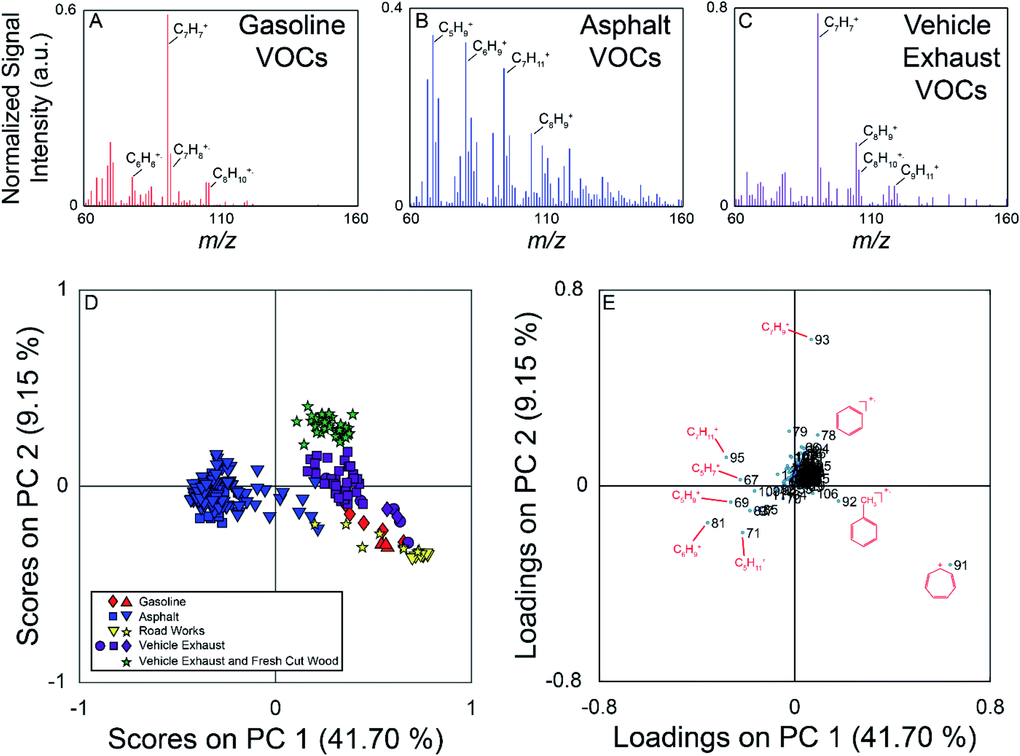 | ||
| Fig. 2 Top: Example full scan MIMS spectra collected near fresh gasoline (A), freshly laid asphalt (B), and vehicle exhaust (C). Some ions of interest have been labeled on each mass spectrum. (Panel D) PC 1 versus PC 2 scores plot of the full scan MIMS data. Samples (based on mass spectra averaged for 15 s) are coloured based on their source type (asphalt – blue, gasoline – red, vehicle exhaust – purple, vehicle exhaust mixed with sawmill emissions – green, other road works – yellow), and the shapes represent different events when the source was encountered. (Panel E) PC 1 versus PC 2 loadings plot for the MIMS analysis. The separation of asphalt samples in the scores plot is driven by the ions with negative loadings on PC 1. These ions were measured with higher relative abundance in the asphalt samples. | ||
The PCA for the MIMS data is shown in Fig. 2, with the scores plot shown in panel D, and the loadings plot in panel E. For this dataset, PC 1 describes 42% of the variance, PC 2 describes 9%, and PC 3 describes 6%. The variance captured by each of the PCs can be visualized using a Scree plot, in which the relative variances are plotted in descending order. The Scree plot for this analysis is shown in Fig. S3 in the ESI† indicating that the first 10 PCs account for 71% of the variance in the data. Samples in the scores plot are colour-coded based on nearby sources identified in the field notes, and samples from similar hydrocarbon sources are seen clustered together. PC 1 discriminates the asphalt samples from the other measured samples. The asphalt samples generally have negative scores on PC 1 and scores close to zero on PC 2. PC 2 allows for the discrimination of vehicle exhaust from fugitive emissions from gasoline and road works samples. Generally, the vehicle exhaust samples have more positive scores on PC 2. The aged gasoline samples (red diamonds) have more positive scores than the fresh gasoline samples (red triangles) on PC 1. Weathering of gasoline samples leads to the loss of the more volatile compounds which could account for the separation of the fresh and aged gasoline samples.53 The samples associated with other road works activities plot near the gasoline samples. We hypothesize that these samples could have been influenced by fugitive emissions from hydrocarbon cleaning mixtures or improperly sealed gasoline containers. For the vehicle exhaust samples, the samples with the highest positive scores on PC 2 were collected across the street from a sawmill as vehicles were unloading from a ferry. These samples are also impacted by emissions from the sawmill, discriminating them from samples impacted solely by vehicle exhaust observed elsewhere. It was not possible for us to sample air impacted only by the sawmill without the confounding influence of vehicle exhaust on this field campaign. The scores plot for PC 1 versus PC 3 is found in Fig. S4 (panel A) in the ESI.† In this projection, the asphalt samples remain well separated, with negative scores on PC 1, but there is more overlap between the other hydrocarbon samples.
The loadings plot identifies which m/z lead to sample discrimination in the scores plot. Many of the measured m/z that are more dominant in the asphalt mass spectrum have negative loadings on PC 1, while m/z 91 demonstrates a high positive loading on PC 1, and was the base peak in most of the mass spectra from other sources. Ions due to the presence of α-pinene or other monoterpenes (m/z 93 (C7H9+) and 136 (C10H16+)) from fresh cut forest products have positive loadings on PC 2 allowing the vehicle exhaust samples collected near a sawmill to be discriminated from those collected elsewhere in the region. The loadings plot for PC 1 versus PC 3 is found in Fig. S4† (panel B), and indicates that it is once again the asphalt samples that are differentiated from the others due to a greater number of observed compounds. Overall, this analysis demonstrates that full scan MIMS data of ambient, volatile organic hydrocarbons collected while driving can be used to discriminate samples arising from different sources.
Proton-transfer reaction time-of-flight mass spectrometry
PTR-ToF-MS is more sensitive to a wider range of polar and non-polar VOCs than MIMS as well as being more selective due to the significantly greater mass resolution. Consequently, more compounds were observed during the August 2017 field campaign. Samples were collected from both stationary (e.g., industrial sites, transportation infrastructure) and moving sources (wood chip truck, farm vehicles).A total of 290 peaks were identified between m/z 30–215 in the full scan data. Table S5 in the ESI† provides a peak list of the major ions detected in the field campaign, with our measured m/z, possible chemical formula, calculated exact mass for the formula, potential compound identities, and observed sources. The range of compounds detected included hydrocarbons (e.g., BTEX, isoprene, monoterpenes), oxygenated species (e.g., methanol, acetone, acetaldehyde), and sulfur compounds (e.g., dimethyl sulfide). As the PTR-ToF-MS does not employ chromatography or tandem mass spectrometry for additional selectivity, isomers cannot be distinguished, and the signal intensity of each m/z is for the sum of isomers (e.g., m/z 59.048 would have a chemical formula of C3H7O+ which could be both protonated acetone and protonated propanal). It should be noted that peaks at m/z 93.036, 107.076, 121.085, and 135.092, attributed to the protonated molecular ions of hydrocarbons associated with fugitive emissions and/or incomplete combustion of fossil fuels, have also been observed to be derived from the fragmentation of mono and sesquiterpenes, even with the softer chemical ionization of proton transfer.54,55 This is reflected in the listed sources for these ions, as these ions had major sources near an auto wrecking facility, gas station, and ferry, but were also detected near biomass sources such as the sawmills, composting facilities, and a wood chip truck. For the purpose of the analysis described below the different samples have been broadly classified as follows: aged biomass samples–samples collected near a landfill, municipal composting facility, and topsoil producers; fresh biomass samples–samples collected near sawmills, wood chip trucks, wood storage, and sawdust piles; hydrocarbon samples–samples collected near a gas station, ferry terminal, and auto wrecking facility; pulp mill samples–samples collected near two pulp mills; and the farm vehicle samples were collected near a tractor carrying hay.
During the 2017 campaign there were several compounds measured exclusively at or near particular sources. For example, m/z 63.022 (C2H7S+) was only detected near the two pulp mills on the drive route. Peaks at m/z 57.070 (C4H9+), 107.076 (C8H11+), and 121.085 (C9H13+) were generally detected near a gas station, ferry, and an auto wrecking facility. Example mass spectra are shown in Fig. 3 (panels A–C), with some ions of interest labeled on the mass spectra. The mass spectrum in panel A was collected near the municipal composting facility, the mass spectrum in panel B was collected near the auto wrecker, and the mass spectrum shown in panel C was collected near a sawmill. The mass spectrum collected near the auto wrecker is dominated by hydrocarbons, while the mass spectra collected near the compost and sawmill also contain ions for oxygenated species.
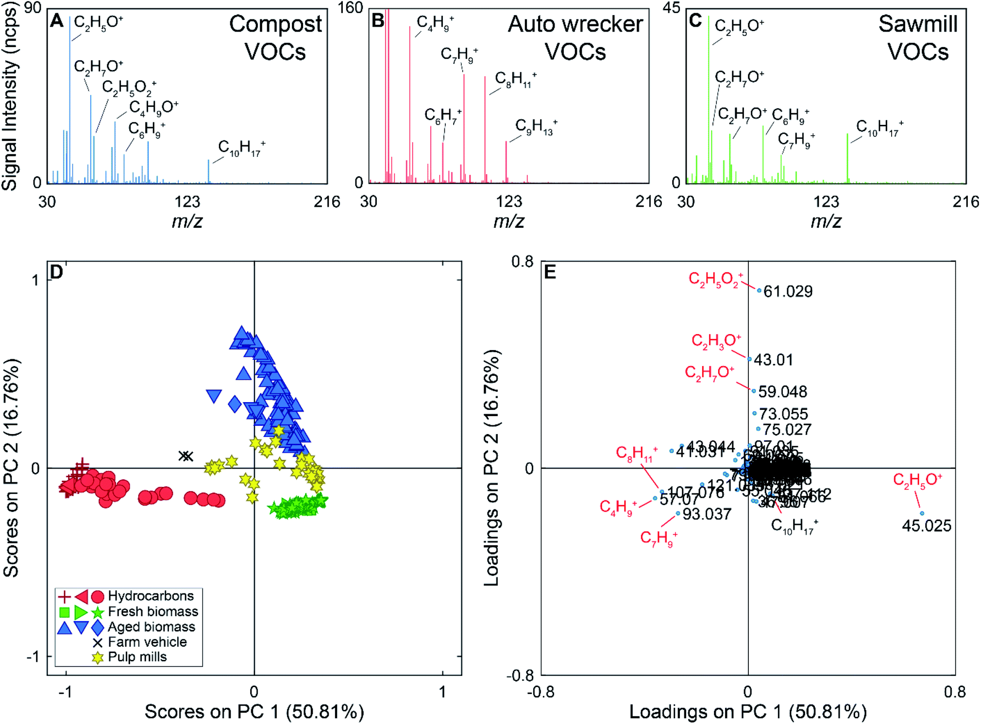 | ||
| Fig. 3 Top: Example full scan PTR-ToF-MS mass spectra collected near a composting facility (A), auto wrecking facility (B), and sawmill (C). Some ions of interest have been labelled on each mass spectra. (Panel D) PC 1 versus PC 2 scores plot of the full scan PTR-ToF-MS data. Red samples are from hydrocarbon sources, blue samples from aged biomass sources, green samples from fresh biomass sources, yellow samples from pulp mills (both fresh and processed biomass), and black samples were collected near a tractor carrying hay (hydrocarbon and biomass source). The different shapes represent different sources (e.g., red stars are near a ferry, red diamonds are near an auto wrecking facility, and red circles are near a gas station). Hydrocarbon samples (red) can be discriminated from biomass samples based on the scores on PC 1. PC 2 discriminates aged biomass samples from fresh biomass. (Panel E) PC 1 versus PC 2 loadings plot of the PTR-ToF-MS data. Ions associated with alkylated aromatic compounds (m/z 93.061, 107.076, and 121.085) allow for the discrimination of hydrocarbon sources from biomass sources due to their negative loading on PC 1. Along PC 2, acetic acid (m/z 61.029) has a high positive loading, while acetaldehyde (m/z 45.025) and monoterpenes (m/z 137.112) have negative loadings leading to the separation of fresh and aged biomass sources. | ||
For the supervised PCA, 298 average mass spectra were used. The PCA scores and loadings plots for the PTR-ToF-MS data are shown in Fig. 3 (panels D and E). PC 1 accounts for 51% of the variance in the data set, with PC 2 accounting for 17%. The Scree plot for the analysis is shown in Fig. S5 in the ESI† with the first three PCs accounting for 78% of the variance in the data set (>97% of the variance is described by the first 10 PCs). Samples in the scores plot have been colour-coded based on the source type they represent (e.g., hydrocarbon, fresh biomass), and the different shapes of the same colour indicate different encounters with the same source type. For example, we encountered three primarily hydrocarbon sources (red) and they are marked as triangles (ferry), plus signs (auto wrecking facility), and circles (gas station) in Fig. 3. In the scores plot, hydrocarbon samples have negative scores on PC 1, discriminating them from other source types. PC 2 provides discrimination between VOCs from fresh biomass, pulp mills, and aged biomass samples. The latter have positive scores on PC 2, samples with scores near zero on PC 2 are associated with pulp mill emissions, and samples with negative scores on PC 2 are due to emissions from fresh biomass near sawmills, wood chip trucks, etc. Additionally, samples collected near a farm vehicle carrying hay are located between the hydrocarbon and biomass samples on the scores plot, potentially due to the mixed nature of this source.
The loadings plot can be used to identify possible compounds leading to sample discrimination. For example, the [MH]+ ions for many hydrocarbons (m/z 93.061, 107.076, 121.084) have negative loadings on PC 1, which allows the hydrocarbon samples to be discriminated from the biogenic emissions. Acetaldehyde (m/z 45.025) has a negative loading on PC 2, while acetic acid (m/z 61.029) which was mainly detected in the vicinity of the compost facility has the highest positive loading on PC 2.
The PCA showing the scores and loadings for PC 1 versus PC 3 are shown in Fig. S6 in the ESI.† In this projection, the hydrocarbon samples are still separated from the biomass samples, as that discrimination falls along PC 1, but there is more overlap between the biomass and pulp mill samples. Some of the pulp mill samples have high positive scores on PC 3 due to the presence of dimethyl sulphide (m/z 63.022) in these samples.
The mass spectra used for this analysis did not include the signal intensity for protonated methanol as this improved sample discrimination for samples impacted by biomass sources and removed the confounding influence of detecting periodic windshield washing fluid from vehicles during on-road sampling. The PCA including methanol is shown in Fig. S7 in the ESI.† When methanol is included, hydrocarbon sources remain well separated, but there is some overlap between the pulp mill and fresh biomass samples and the samples associated with pulp mills and aged biomass sources overlap completely.
A regional scale map of the samples is shown in the top panel of Fig. 4 along with the time series of the data (bottom panel). The drive route is shown by the black line, with the samples used in the supervised PCA colour-coded based on source type. The size of the dot is scaled by the total VOC concentration using the total ion current for m/z 30–215 (excluding the reagent ions). The labels on the map show the nearby VOC sources. Those labeled in black text are stationary sources (mostly industrial), and those labeled in red text were moving. The time series data shows the overlay of all measured m/z observed during the field campaign, with the exception of methanol (as it was excluded from the chemometric analysis). Mass spectral peaks of interest are labelled on the time series, and the portions of the time series data collected near the identifiable sources used in the PCA are indicated by the coloured bars along the top of the plot. Fig. S8 (panels A–D) in the ESI† show time series of subsets of the measured compounds, with methanol in panel A, major hydrocarbon ions and their fragments in panel B, major non-methanol oxygenated species and their fragments in panel C, and sulphur compounds in panel D. It is also important to note that the on-road measurements can be influenced by mobile sources and are not always associated with stationary area sources. With the exception of acetic acid (which exhibits a slow decay time due to carry-over in the sample line), we observe only small differences in the decay times of the remaining VOCs described here (<5 s). These differences are dampened out for the supervised analysis (15 s averaged mass spectra) and have only a minor influence on the unsupervised analysis using 1 second averaged mass spectra. In both cases, the decay times do not change the distribution of identified sources at the spatial resolution presented here.
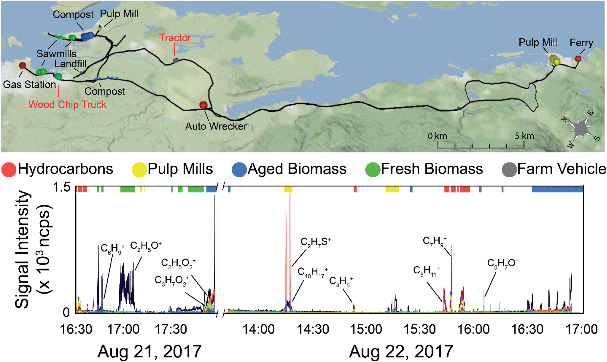 | ||
| Fig. 4 Top: Map of samples used in the PTR-ToF-MS analysis allowing the spatial distribution of the samples to be visualized. The size of the dots are proportional to total VOC concentration encapsulating the 40th, 60th, and 80th percentiles of the total ion current for the 298 samples used in the PCA. The dots are colour-coded based on sample source (red – hydrocarbons, yellow – pulp mills, blue – aged biomass, green – fresh wood, grey – farm vehicle). Bottom: Time series of all the m/z measured on August 21 shown on the left of the x-axis cut, and August 22, shown on the right. The coloured bars on the top of the graph indicated which data was used in the supervised PTR-ToF-MS analysis and are coloured based on source type. | ||
Given the success of discriminating known VOC samples above, we have extended this method to identify groupings within the full data set in an unsupervised analysis. The complete dataset contains 16737 mass spectra measured at 1 second intervals across 290 mass channels. As has been noted by others, the high sample-to-variable ratio reduces the likelihood of spurious correlations.56 Two clustering algorithms (GMM and DBSCAN) were employed to group samples based solely on their mass spectral fingerprints. The GMM algorithm clusters all data points into groups, whereas DBSCAN only assigns dense data clusters within the PCA model. A PCA model was used as the algorithm input as this greatly reduced computational time, especially in the case of the GMM. A 15 component PCA model was used as the input. The first three PCs represent 44% of the variance in the dataset. Most PCs past the 10th, modelled noise, with only a few beyond that showing some structure related to specific geographic locations (i.e., PCs 12 and 15). The 15 PC model describes 79% of the variance in the data, with each subsequent PC accounting for less than 1.2% of the variance. It was also found that the addition of more PCs had little impact on the results of the clustering algorithms (data not shown).
For the calculated GMMs both the AIC and BIC values were minimized using unshared, full covariance matrices for 2–20 clusters. For these models, the AIC and BIC values decreased with increasing cluster number, with very similar values obtained for 12–20 clusters. Additional AIC and BIC values were calculated for up to 40 clusters using the models with full, unshared covariance matrices. The plots of the AIC and BIC values are found in Fig. S9 of the ESI.† The calculated AIC values are similar for models using 12 or more clusters (they continue to decrease up to 40 clusters), whereas the BIC values reach a minimum value at 27 clusters. As BIC penalizes model complexity more than AIC,46 the BIC minimum value of 27 was used as an indicator of the most complex model needed to describe the data, with models containing 9, 10, 11, 12, 13 and 14 clusters also being calculated. Geospatial maps of the different models were compared, and the 12 group model was selected as it was able to identify sources within the dataset, without overcomplicating the model.
The PCA scores plots of PC 1 versus PC 2 and PC 1 versus PC 3 for this analysis are shown in Fig. 5 (panels A and B), with a map of the results in Fig. 5 (panel C). Many of the point sources on the map are identified by the large dots in their vicinity (gas station, compost facility, ferry terminal, pulp mill, auto wrecker). Samples are coloured based on group membership as determined by the 12 group GMM. Fig. S10 in the ESI† show the loadings plots of PC 1 versus PC 2 and PC 1 versus PC 3 in panels A and B respectively. In the scores plots similar samples are grouped together, with many point sources grouping along the corners and edges of the data. Groups with individual sources or source types have been identified on the scores plot. For clarity, Fig. S11† (panels A–L) depicts the PC 1 versus PC 2 scores plots for the individual groups, as well as the average mass spectra for each of the groups with some ions of interest labeled. Scores along PC 2 discriminate hydrocarbon sources from pulp mill samples, fresh, and aged biomass samples. PC 1 can be used to discriminate the biomass sources, with aged biomass having negative scores on PC 1 and fresh biomass having positive scores on PC 1.
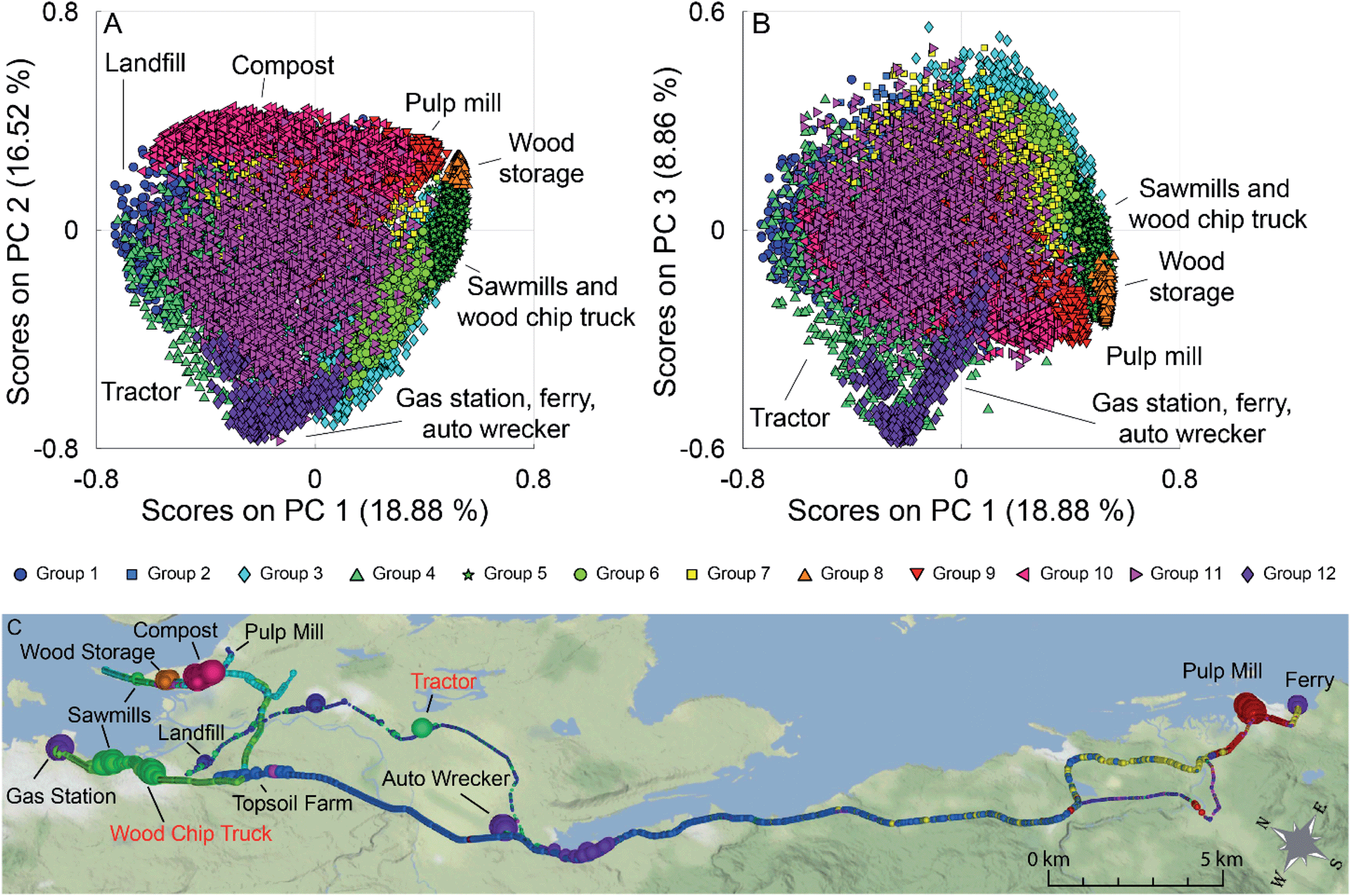 | ||
| Fig. 5 (A) PCA scores plot for PC 1 versus PC 2. (B) PCA scores plot for PC 1 versus PC 3. Samples are coloured based on the groups identified using the GMM algorithm. Some groups containing individual VOC sources (such as the municipal compost facility, and one of the pulp mills) or multiple VOC sources of the same type (e.g., sawmill emissions are grouped with the samples from the wood chip truck) are labeled. (C) Geospatial map showing the spatial distribution of the samples, with dot size proportional to total VOC concentration. Locations of interest are labelled, with moving sources being represented by red text. | ||
The loadings plots shown in Fig. S10† (panels A and B) indicates that similar ions lead to sample discrimination in the supervised and unsupervised data sets, with signals associated with acetic acid, acetaldehyde, formic acid/ethanol, ethylbenzene/xylenes, and toluene having high loadings. For the groups identified using GMM, some groups were associated with a single source, while others contained samples from multiple sources. For example, Group 10 (magenta triangles) was only measured near a municipal composting facility with a mass spectrum dominated by a C2H3O+ ester or acid fragment, acetaldehyde, acetone, acetic acid, and monoterpenes signals (Fig. S11,† panel J) while Group 9 (red triangles) was collected mainly in the vicinity of a pulp mill with signals associated with acetaldehyde, acetone, acetic acid, dimethyl sulfide, and monoterpenes (Fig. S11,† panel I). Other groups were associated with multiple sources with similar emissions. For example, Group 5 contained samples collected near multiple sawmills, and from driving near a wood chip truck with a mass spectrum influenced by acetaldehyde and monoterpene fragments (Fig. S11,† panel E); and Group 12 is impacted by the three hydrocarbon sources, and an unknown source, with a mass spectrum dominated by the BTEX suite and other alkylated aromatics (Fig. S11,† panel L). Finally, some sources are present in multiple groups in the scores plot. For example, a group of pulp mill samples has positive scores on PC 1 and PC 2 (Group 9, red triangles), while other pulp mill samples are have positive scores on PC 1 and negative scores on PC 2 (Group 3, blue diamonds). As pulp mills have multiple different sources for VOC emissions (e.g., wood chip piles, pulp production, wastewater ponds), it is not surprising that not all the pulp mill samples are grouped together. Some VOC sources encountered during the field campaigns were unidentified at the time of sampling as can be seen in the grey shaded areas in Fig. 1. We have tentatively assigned source classes to these VOC signals based on the group membership in the unsupervised data analysis. For example, the unidentified signals that appear at 16:40 in Fig. 1 could be attributed to a hydrocarbon source, whereas those at 16:53 and 17:15–17:25 could be assigned to pulp mill emissions. The assignment of the samples collected from 17:15–17:25 is supported by field observations noting a sulfur smell. Given the limited data presented here, we have chosen not to build a classification model. Future field campaigns will include more sources and replicates to enable us to train and verify a robust predictive model.
For the DBSCAN analysis a neighbourhood size of 0.022 was used with 9 neighbours being needed to identify core points. This algorithm identified 13 groups within the data (1 of which, Group 13, represents data that was not clustered). Unlike the GMM algorithm, DBSCAN has not assigned all data points to a cluster, however it has identified most of the high VOC concentration samples within the dataset. The results of the analysis are seen in Fig. S12,† with the PC 1 versus PC 2 and PC 1 versus PC 3 scores plots shown in panels A and B, and maps of the analysis shown in panels C and D. The data is coloured by the DBSCAN group membership, with the black dots representing the data left ungrouped. The map in Fig. S12† (panel C) shows all data, while the map in Fig. S12† (panel D) omits the black data points for clarity. The PC 1 versus PC 2 scores plots and average mass spectra for each of the groups is shown in Fig. S13 (panels A–M) in the ESI.† Samples are clustered based on source type, with most of the clusters falling on the extremities of the scores plot. Group 8 (Fig. S13,† panel H), which has scores near the origin on each of the three PCs shown contains high concentration samples measured in the vicinity of a pulp mill at approximately 14:15 on August 22, 2017. These samples were higher in dimethyl sulfide (m/z 63.022) than those measured elsewhere, but dimethyl sulfide does not have a significant loading until higher PCs (e.g., PCs 6, 7, 12, and 15 (data not shown)). Groups 2, 4, 5, 8, and 12 (Fig. S13,† panels B, D, E, and L) have identified single sources within the data (gas station, wood chip truck, compost, pulp mill, and an unknown (possibly hydrocarbon) source respectively), while groups 3 and 10 (Fig. S13,† panels C and J) contain samples from multiple sources of similar type (fresh biomass samples and hydrocarbon samples).
In some cases, the clusters identified by GMM have also been identified by DBSCAN, while in other cases DBSCAN has identified multiple clusters within a single group identified by GMM. For example, GMM Group 10 (Fig. S11,† panel J) and DBSCAN Group 5 (Fig. S13,† panel E) contain almost the same set of samples. The mass spectra associated with them have a correlation coefficient of 0.999 (Table S6†). In the case of GMM Group 12 (Fig. S11,† panel L), the DBSCAN has identified 3 sub-clusters (Fig. S13,† panels B, J, and L) with correlation coefficients between the identified mass spectra of 0.916, 0.990, and 0.604 for DBSCAN Groups 2, 10, and 12, respectively. In this case, DBSCAN has separately identified different hydrocarbon sources described by mass spectra containing different ratios of the measured hydrocarbons, while GMM has identified one cluster containing all the hydrocarbon samples. A full correlation matrix between the mass spectra for the clusters identified by the two methods is shown in Table S6.†
The purpose of the unsupervised analysis done using both GMM and DBSCAN algorithms was not to construct a definitive model of the data collected, but to demonstrate the ability of the techniques to identify different VOC sources measured using a PTR-ToF-MS operated in a moving vehicle. Both techniques were able to discriminate VOC sources using the normalized mass spectal fingerprint and associate these sources with specific geographic locations.
Conclusions
The work presented here represents the first application of chemometric analysis to mobilized direct mass spectrometry for VOC source discrimination and fine scale spatial distribution mapping. Supervised PCA analysis of normalized full scan mass spectra provide meaningful sample discrimination and an unsupervised analysis uncovers additional VOC source assignments. We demonstrate the use of MIMS to discriminate various hydrocarbon sources. The PTR-ToF-MS instrument is not constrained to small hydrophobic molecules and is generally more sensitive and selective, providing a richer dataset inclusive of more polar VOCs including those often associated with nuisance odours. Consequently, it can be used to discriminate samples from a wider range of sources. The data is displayed on a geospatial map for visualization and further interrogation. The use of non-targeted full scan mass spectral data without determining the concentrations of individual VOCs reduces the amount of data processing and will facilitate real-time source identification.Mass spectrometry yields molecular level information about the sample composition, which provides chemical insight that can be used to inform targeted analysis, or be used to identify molecular markers. Although the analysis presented here cannot identify VOC sources that have not been previously encountered, it will direct the user to ‘unknowns’, which can be the subject of subsequent investigation. Future work includes the application of data fusion techniques to improve source discriminating power by incorporating data from inorganic gas and particulate matter sensors. The incorporation of this data into a Geographic Information System will allow us to map plume boundaries and inform dispersion models. We are currently exploring Positive Matrix Factorization and Multivariate Curve Resolution – Alternating Least Squares to identify sources contributing at each sampling location and apportion their relative contributions to ambient air samples.
Conflicts of interest
There are no conflicts to declare.Acknowledgements
The authors gratefully acknowledge Vancouver Island University and the University of Victoria for ongoing support of the Applied Environmental Research Laboratories and Graduate Student Researchers. The mobile mass spectrometry lab was made possible with the support of the Canada Foundation for Innovation (CFI32238) and the British Columbia Knowledge Development Fund. The research was supported through the Natural Sciences and Engineering Research Council of Canada (NSERC Discovery Grant 2016-06454), the Fraser Basin Council supported the project through their BC Clean Air Research Fund, and the MITACS Accelerate Program.References
- R. G. Derwent, Sources, Distributions, and Fates of VOCs in the Atmosphere, Volatile Org. Compd. Atmos., 1995, 1–15 CAS.
- Environment and Climate Change Canada, Volatile Organic Compounds in Consumer and Commercial Products, http://www.ec.gc.ca/cov-voc/, accessed 23 February 2017 Search PubMed.
- United States Environmental Protection Agency, Volatile Organic Compounds' Impact on Indoor Air Quality, https://www.epa.gov/indoor-air-quality-iaq/volatile-organic-compounds-impact-indoor-air-quality, accessed 23 February 2017 Search PubMed.
- P. S. Monks, Gas-phase radical chemistry in the troposphere, Chem. Soc. Rev., 2005, 34, 376–395 RSC.
- P. J. Ziemann and R. Atkinson, Kinetics, products, and mechanisms of secondary organic aerosol formation, Chem. Soc. Rev., 2012, 41, 6582–6605 RSC.
- World Health Organization Public Health and Environment, Exposure To Benzene: A Major Public Health Concern, Geneva, 2010 Search PubMed.
- J. H. Seinfeld and S. N. Pandis, Atmospheric chemistry and physics: from air pollution to climate change, John Wiley & Sons, Hoboken, New Jersey, 3rd edn, 2016 Search PubMed.
- I. J. Simpson, N. J. Blake, B. Barletta, G. S. Diskin, H. E. Fuelberg, K. Gorham, L. G. Huey, S. Meinardi, F. S. Rowland, S. A. Vay, A. J. Weinheimer, M. Yang and D. R. Blake, Characterization of trace gases measured over Alberta oil sands mining operations: 76 speciated C 2 – C 10 volatile organic compounds (VOCs), CO2, CH4, CO, NO, NO2, NOy, O3, and SO2, Atmos. Chem. Phys., 2010, 10, 11931–11954 CrossRef CAS.
- United States Environmental Protection Agency, Method TO-17: Determination of Volatile Organic Compounds in Ambient Air Using Active Sampling Onto Sorbent Tubes, EPA Methods, 1999, pp. 1–53 Search PubMed.
- Y. Liu, Q. Xie, X. Li, F. Tian, X. Qiao, J. Chen and W. Ding, Profile and source apportionment of volatile organic compounds from a complex industrial park, Environ. Sci.: Processes Impacts, 2019, 21, 9–18 RSC.
- L. Cui, Z. Zhang, Y. Huang, S. C. Lee, D. R. Blake, K. F. Ho, B. Wang, Y. Gao, X. M. Wang and P. K. K. Louie, Measuring OVOCs and VOCs by PTR-MS in an urban roadside microenvironment of Hong Kong: Relative humidity and temperature dependence, and field intercomparisons, Atmos. Meas. Tech., 2016, 9, 5763–5779 CrossRef CAS.
- C. Sarkar, V. Sinha, B. Sinha, A. K. Panday, M. Rupakheti and M. G. Lawrence, Source apportionment of NMVOCs in the Kathmandu Valley during the SusKat-ABC international field campaign using positive matrix factorization, Atmos. Chem. Phys., 2017, 17, 8129–8156 CrossRef CAS.
- C. Kaltsonoudis, E. Kostenidou, K. Florou, M. Psichoudaki and S. N. Pandis, Temporal variability and sources of VOCs in urban areas of the eastern Mediterranean, Atmos. Chem. Phys., 2016, 16, 14825–14842 CrossRef CAS.
- L. Kaser, T. Karl, A. Guenther, M. Graus, R. Schnitzhofer, A. Turnipseed, L. Fischer, P. Harley, M. Madronich, D. Gochis, F. N. Keutsch and A. Hansel, Undisturbed and disturbed above canopy ponderosa pine emissions: PTR-TOF-MS measurements and MEGAN 2.1 model results, Atmos. Chem. Phys., 2013, 13, 11935–11947 CrossRef.
- B. Yuan, A. R. Koss, C. Warneke, M. Coggon, K. Sekimoto and J. A. de Gouw, Proton-Transfer-Reaction Mass Spectrometry: Applications in Atmospheric Sciences, Chem. Rev., 2017, 13187–13229 CrossRef CAS PubMed.
- C. Song, B. Liu, Q. Dai, H. Li and H. Mao, Temperature dependence and source apportionment of volatile organic compounds (VOCs) at an urban site on the north China plain, Atmos. Environ., 2019, 207, 167–181 CrossRef CAS.
- J. Li, Y. Hao, M. Simayi, Y. Shi, Z. Xi and S. Xie, Verification of anthropogenic VOC emission inventory through ambient measurements and satellite retrievals, Atmos. Chem. Phys. Discuss., 2019, 1–31 Search PubMed.
- T. W. Tokarek, C. A. Odame-Ankrah, J. A. Huo, R. McLaren, A. K. Y. Lee, M. G. Adam, M. D. Willis, J. P. D. Abbatt, C. Mihele, A. Darlington, R. L. Mittermeier, K. Strawbridge, K. L. Hayden, J. S. Olfert, E. G. Schnitzler, D. K. Brownsey, F. V. Assad, G. R. Wentworth, A. G. Tevlin, D. E. J. Worthy, S. M. Li, J. Liggio, J. R. Brook and H. D. Osthoff, Principal component analysis of summertime ground site measurements in the Athabasca oil sands with a focus on analytically unresolved intermediate-volatility organic compounds, Atmos. Chem. Phys., 2018, 18, 17819–17841 CrossRef CAS.
- R. J. Bell, N. G. Davey, M. Martinsen, C. Collin-Hansen, E. T. Krogh and C. G. Gill, A field-portable membrane introduction mass spectrometer for real-time quantitation and spatial mapping of atmospheric and aqueous contaminants, J. Am. Soc. Mass Spectrom., 2015, 26, 212–223 CrossRef CAS PubMed.
- Z. L. Hildenbrand, P. M. Mach, E. M. McBride, M. N. Dorreyatim, J. T. Taylor, D. D. Carlton, J. M. Meik, B. E. Fontenot, K. C. Wright, K. A. Schug and G. F. Verbeck, Point source attribution of ambient contamination events near unconventional oil and gas development, Sci. Total Environ., 2016, 573, 382–388 CrossRef CAS PubMed.
- P. M. Mach, E. M. Mcbride, Z. J. Sasiene, K. R. Brigance, S. K. Kennard, K. C. Wright and G. F. Verbeck, Vehicle-Mounted Portable Mass Spectrometry System for the Covert Detection via Spatial Analysis of Clandestine Methamphetamine Laboratories, Anal. Chem., 2015, 87, 11501–11508 CrossRef CAS PubMed.
- N. G. Davey, C. T. E. Fitzpatrick, J. M. Etzkorn, M. Martinsen, R. S. Crampton, G. D. Onstad, T. V. Larson, M. G. Yost, E. T. Krogh, M. Gilroy, K. H. Himes, E. T. Saganić, C. D. Simpson and C. G. Gill, Measurement of spatial and temporal variation in volatile hazardous air pollutants in Tacoma, Washington, using a mobile membrane introduction mass spectrometry (MIMS) system, J. Environ. Sci. Health, Part A: Toxic/Hazard. Subst. Environ. Eng., 2014, 49, 1199–1208 CrossRef CAS PubMed.
- M. Zavala, S. C. Herndon, E. C. Wood, J. T. Jayne, D. D. Nelson, A. M. Trimborn, E. Dunlea, W. B. Knighton, A. Mendoza, D. T. Allen, C. E. Kolb, M. J. Molina and L. T. Molina, Comparison of emissions from on-road sources using a mobile laboratory under various driving and operational sampling modes, Atmos. Chem. Phys., 2009, 9, 1–14 CrossRef CAS.
- R. J. Bell, R. T. Short and R. H. Byrne, In situ determination of total dissolved inorganic carbon by underwater membrane introduction mass spectrometry, Limnol. Oceanogr.: Methods, 2011, 9, 164–175 CrossRef CAS.
- R. T. Short, S. K. Toler, G. P. G. Kibelka, D. T. Rueda Roa, R. J. Bell and R. H. Byrne, Detection and quantification of chemical plumes using a portable underwater membrane introduction mass spectrometer, TrAC, Trends Anal. Chem., 2006, 25, 637–646 CrossRef CAS.
- M. Müller, T. Mikoviny, S. Feil, S. Haidacher, G. Hanel, E. Hartungen, A. Jordan, L. Märk, P. Mutschlechner, R. Schottkowsky, P. Sulzer, J. H. Crawford and A. Wisthaler, A compact PTR-ToF-MS instrument for airborne measurements of volatile organic compounds at high spatiotemporal resolution, Atmos. Meas. Tech., 2014, 7, 3763–3772 CrossRef.
- B. Yuan, A. Koss, C. Warneke, J. B. Gilman, B. M. Lerner, H. Stark and J. A. De Gouw, A high-resolution time-of-flight chemical ionization mass spectrometer utilizing hydronium ions (H3O+ ToF-CIMS) for measurements of volatile organic compounds in the atmosphere, Atmos. Meas. Tech., 2016, 9, 2735–2752 CrossRef CAS.
- L. C. Richards, N. G. Davey, T. F. Fyles, C. G. Gill and E. T. Krogh, Discrimination of constructed air samples using multivariate analysis of full scan membrane introduction mass spectrometry (MIMS) data, Rapid Commun. Mass Spectrom., 2018, 32, 349–360 CrossRef CAS PubMed.
- R. A. Ketola, T. Kotiaho, M. E. Cisper and T. M. Allen, Environmental applications of membrane introduction mass spectrometry, J. Mass Spectrom., 2002, 37, 457–476 CrossRef CAS PubMed.
- N. G. Davey, E. T. Krogh and C. G. Gill, Membrane-introduction mass spectrometry (MIMS), TrAC, Trends Anal. Chem., 2011, 30, 1477–1485 CrossRef CAS.
- E. T. Krogh and C. G. Gill, Membrane introduction mass spectrometry (MIMS): A versatile tool for direct, real-time chemical measurements, J. Mass Spectrom., 2014, 49, 1205–1213 CrossRef CAS PubMed.
- D. Pagonis, K. Sekimoto and J. de Gouw, A Library of Proton-Transfer Reactions of H3O+ Ions Used for Trace Gas Detection, J. Am. Soc. Mass Spectrom., 2019, 30, 1330–1335 CrossRef CAS PubMed.
- R. S. Blake, P. S. Monks and A. M. Ellis, Proton-Transfer Reaction Mass Spectrometry, Chem. Rev., 2009, 109, 861–896 CrossRef CAS PubMed.
- A. Koss, B. Yuan, C. Warneke, J. B. Gilman, B. M. Lerner, P. R. Veres, J. Peischl, S. Eilerman, R. Wild, S. S. Brown, C. R. Thompson, T. Ryerson, T. Hanisco, G. M. Wolfe, J. M. St Clair, M. Thayer, F. N. Keutsch, S. Murphy and J. De Gouw, Observations of VOC emissions and photochemical products over US oil- and gas-producing regions using high-resolution H3O+ CIMS (PTR-ToF-MS), Atmos. Meas. Tech., 2017, 10, 2941–2968 CrossRef CAS.
- P. K. Misztal, T. Karl, R. Weber, H. H. Jonsson, A. B. Guenther and A. H. Goldstein, Airborne flux measurements of biogenic isoprene over California, Atmos. Chem. Phys., 2014, 14, 10631–10647 CrossRef.
- H. Abdi and L. Williams, Principal component analysis, Wiley Interdisciplinary Reviews: Computational Statistics, 2010, 2, 433–459 CrossRef.
- R. Bro and A. K. Smilde, Principal component analysis, Anal. Methods, 2014, 6, 2812–2831 RSC.
- K. P. Wyche, P. S. Monks, K. L. Smallbone, J. F. Hamilton, M. R. Alfarra, A. R. Rickard, G. B. McFiggans, M. E. Jenkin, W. J. Bloss, A. C. Ryan, C. N. Hewitt and A. R. MacKenzie, Mapping gas-phase organic reactivity and concomitant secondary organic aerosol formation: Chemometric dimension reduction techniques for the deconvolution of complex atmospheric data sets, Atmos. Chem. Phys., 2015, 15, 8077–8100 CrossRef CAS.
- L. Cappellin, F. Biasioli, P. M. Granitto, E. Schuhfried, C. Soukoulis, F. Costa, T. D. Märk and F. Gasperi, On data analysis in PTR-TOF-MS: From raw spectra to data mining, Sens. Actuators, B, 2011, 155, 183–190 CrossRef CAS.
- R. Sparrapan, M. N. Eberlin and R. M. Alberici, Natural and artificial markers of gasoline detected by membrane introduction mass spectrometry, Anal. Methods, 2011, 3, 751 RSC.
- R. M. Alberici, C. G. Zampronio, R. J. Poppi and M. N. Eberlin, Water solubilization of ethanol and BTEX from gasoline: on-line monitoring by membrane introduction mass spectrometry, Analyst, 2002, 127, 230–234 RSC.
- R. A. Ketola, J. Heikkonen, S. Piepponen, F. R. Lauritsen and T. Kotiaho, Classification of cola beverages on the basis of mass spectra measured by membrane inlet mass spectrometry, Rapid Commun. Mass Spectrom., 1998, 12, 1011–1017 CrossRef CAS.
- Z. Deuscher, I. Andriot, E. Sémon, M. Repoux, S. Preys, J. M. Roger, R. Boulanger, H. Labouré and J. L. Le Quéré, Volatile compounds profiling by using proton transfer reaction-time of flight-mass spectrometry (PTR-ToF-MS). The case study of dark chocolates organoleptic differences, J. Mass Spectrom., 2019, 54, 92–119 CrossRef CAS PubMed.
- I. Khomenko, I. Stefanini, L. Cappellin, V. Cappelletti, P. Franceschi, D. Cavalieri, T. D. Märk and F. Biasioli, Non-invasive real time monitoring of yeast volatilome by PTR-ToF-MS, Metabolomics, 2017, 13, 1–13 CrossRef CAS PubMed.
- R. J. Bell, N. G. Davey, M. Martinsen, R. T. Short, C. G. Gill and E. T. Krogh, The effect of the earth's and stray magnetic fields on mobile mass spectrometer systems, J. Am. Soc. Mass Spectrom., 2015, 26, 201–211 CrossRef CAS PubMed.
- K. Varmuza and P. Filzmoser, Introduction to Multivariate Statistical Analysis in Chemometrics, CRC Press, Baton Rouge, United States, 2016 Search PubMed.
- J. Han, M. Kamber and J. Pei, Data Mining: Concepts and Techniques, Morgan Kaufmann Publishers, Waltham, MA, 3rd edn, 2012 Search PubMed.
- The Mathworks, Tune Gaussian Mixture Models, https://www.mathworks.com/help/stats/tune-gaussian-mixture-models.html, accessed 15 June 2019 Search PubMed.
- M. Loetzsch, Komoot Outdoor in Google Earth, http://ge-map-overlays.appspot.com/openstreetmap/komoot-outdoor, accessed 15 July 2019 Search PubMed.
- P. D. Wentzell, C. C. Wicks, J. W. B. Braga, L. F. Soares, T. C. M. Pastore, V. T. R. Coradin and F. Davrieux, Implications of measurement error structure on the visualization of multivariate chemical data: Hazards and alternatives, Can. J. Chem., 2018, 96, 738–748 CrossRef CAS.
- J. H. Gross, in Mass Spectrometry: A Textbook, Springer International Publishing, Cham, 2017, pp. 325–437 Search PubMed.
- F. Autelitano, F. Bianchi and F. Giuliani, Airborne emissions of asphalt/wax blends for warm mix asphalt production, J. Cleaner Prod., 2017, 164, 749–756 CrossRef CAS.
- T. J. Bruno and S. Allen, Weathering patterns of ignitable liquids with the advanced distillation curve method, J. Res. Natl. Inst. Stand. Technol., 2013, 118, 29–51 CrossRef CAS PubMed.
- E. Kari, P. Miettinen, P. Yli-Pirilä, A. Virtanen and C. L. Faiola, PTR-ToF-MS product ion distributions and humidity-dependence of biogenic volatile organic compounds, Int. J. Mass Spectrom., 2018, 430, 87–97 CrossRef CAS.
- C. Taiti, C. Costa, W. Guidi Nissim, S. Bibbiani, E. Azzarello, E. Masi, C. Pandolfi, F. Pallottino, P. Menesatti and S. Mancuso, Assessing VOC emission by different wood cores using the PTR-ToF-MS technology, Wood Sci. Technol., 2017, 51, 273–295 CrossRef CAS.
- A. Amann, B. D. L. Costello, W. Miekisch, J. Schubert, B. Buszewski, J. Pleil, N. Ratcliffe and T. Risby, The human volatilome: Volatile organic compounds (VOCs) in exhaled breath, skin emanations, urine, feces and saliva, J. Breath Res., 2014, 8(3), 034001 CrossRef PubMed.
Footnote |
| † Electronic supplementary information (ESI) available. See DOI: 10.1039/c9em00439d |
| This journal is © The Royal Society of Chemistry 2020 |