
 Open Access Article
 This Open Access Article is licensed under a
 Creative Commons Attribution 3.0 Unported Licence
In situ observation of pH change during water splitting in neutral pH conditions: impact of natural convection driven by buoyancy effects†
Keisuke
Obata
 a,
Roel
van de Krol
ab,
Michael
Schwarze
bc,
Reinhard
Schomäcker
b and
Fatwa F.
Abdi
*a
a,
Roel
van de Krol
ab,
Michael
Schwarze
bc,
Reinhard
Schomäcker
b and
Fatwa F.
Abdi
*a
aInstitute for Solar Fuels, Helmholtz-Zentrum Berlin für Materialien und Energie GmbH, Hahn-Meitner-Platz 1, 14109 Berlin, Germany. E-mail: fatwa.abdi@helmholtz-berlin.de
bTechnische Universität Berlin, Department of Chemistry, Straße des 17. Juni 124, 10623, Berlin, Germany
cTechnische Universität Berlin, Department of Process Engineering, Straße des 17. Juni 135, 10623, Berlin, Germany
First published on 3rd November 2020
Abstract
Photoelectrochemical water splitting in near-neutral pH conditions offers a safe and sustainable way to produce solar fuels, but operation at near-neutral pH is challenging because of the added concentration overpotentials due to mass-transport limitations of protons and hydroxide ions. Understanding the extent of this limitation is essential in designing a highly efficient solar fuel conversion device. In the present study, the local pH between the anode and cathode in a water splitting cell is monitored in situ using fluorescence pH sensor foils. By this direct visualization, we confirm that supporting buffer ions effectively suppress local pH changes, and we show that electrochemical reactions induce natural electrolyte convection in a non-stirred cell. The observed electrolyte convection at low current densities (<2 mA cm−2) originates from buoyancy effects due to the change in the local electrolyte density by ion depletion and accumulation. A multiphysics simulation that includes the buoyancy effect reveals that natural convection driven by electrochemical reactions stabilizes the local pH, which is consistent with our experimental observations. In contrast, the model without the buoyancy effect predicts significant shifts of the local pH away from the pKa of the buffer, even at low current densities. This experimentally validated model reveals that natural convection induced by electrochemical reactions significantly affects the overall mass-transport, especially in close vicinity of the electrodes, and it should, therefore, be considered in the design and evaluation of solar fuel conversion devices.
Broader contextSolar water splitting is an attractive approach to overcome the intermittency of sunlight and store it as hydrogen. For a large-scale, stable and safe operation, the use of near-neutral pH solutions is preferred. However, although an efficient (photo)electrocatalyst exists for near-neutral pH operation, the mass-transport limitation of proton and hydroxide ions is a major challenge. Understanding this limitation and how it leads to the formation of pH gradient and the resultant efficiency loss is highly important to devise an efficient design of energy conversion devices, even beyond water splitting (e.g., CO2 reduction). Herein, pH-sensitive fluorescence sensor foils are introduced in an electrochemical cell to monitor the local pH in situ during a water splitting reaction in neutral pH electrolytes. A local pH shift and the appearance of natural convection are clearly visualized. Combined with a multiphysics model, our results show that the natural convection is driven by the change of electrolyte density and plays a significant role to suppress local pH shift. This factor, which is not previously highlighted, should be considered when determining the different design parameters (e.g., flow rate, the choice of anions and cations, product separation strategy) of a (photo)electrochemical device. |
Introduction
The development of solar fuel production technology has attracted increasing interest in the last couple of decades. Such a technology potentially overcomes sunlight's intermittency and allows the storage of solar energy in the form of chemicals, such as hydrogen and hydrocarbons. Various approaches exist, either indirectly by coupling a photovoltaic (PV) cell and an electrolyzer or directly in a suspended photocatalyst particle reactor or a photoelectrochemical (PEC) cell. In the PEC approach, light-absorbing semiconductors (often decorated with electrocatalysts) are immersed in aqueous electrolyte solutions, and electrochemical reactions occur on the surface while the counter-reactions take place on either integrated or wired counter electrodes. Since all functionalities are integrated into a single device, synergistic effects can be expected. For instance, the thermalization of absorbed photons and the thermal energy of sub-bandgap photons will increase the temperature of the system and can improve the electrochemical kinetics and mass-transport in the electrolyte.1–8 Heat transfer from the semiconductor to the electrolyte solution will help to reduce photovoltage losses, especially for temperature-sensitive materials such as Si- and III/V-based semiconductors.8–11 Conversely, higher temperatures may improve charge carrier transport when metal oxide semiconductors with polaronic properties are used.12–15 This is in contrast to PV-coupled electrolyzers, for which the efficiency has been shown to decrease with increasing operating temperature.4 Besides, because the operating current density of a PEC cell is low (<30 mA cm−2) compared to that of commercial electrolyzers (0.5–1.0 A cm−2), lower ohmic and kinetic losses can be expected and the use of noble metal electrocatalysts may be avoided.7,16,17One major challenge in the PEC approach is the instability of many semiconducting materials in electrolyte solutions. This is especially true when extremely acidic or alkaline electrolytes are used, which is the case in commercial electrolyzers. One of the mitigating strategies is to introduce thin protection layers, such as TiO2, on surface of these semiconductors.18–21 However, such layers may suffer from the presence of pinholes and often require expensive deposition techniques, such as atomic layer deposition.22 This limitation, together with safety considerations, drives many researchers to investigate reactions in near-neutral pH electrolytes. These conditions may also enable the use of seawater. However, a serious disadvantage in using near-neutral pH conditions is the low concentration of proton/hydroxide ions in the solution (less than a μmol L−1 around pH 7). At such low concentrations, the reactants will be rapidly depleted during the proton-coupled electron transfer (PCET) reactions and resupply of the reactants from the neighboring electrolyte regions will not be able to keep up due to mass transport limitations. This results in concentration overpotentials in addition to the kinetic overpotentials from electrocatalysts.23–25 Although supporting buffer ions are known to work as proton donors and acceptors, a local pH gradient is still expected to form because of the smaller diffusion coefficients of buffer ions compared to those of proton/hydroxide ions.17,26–30 This effect is even more severe in large-scale devices; it was recently shown that large area PEC devices (≥50 cm2) show much larger local pH shifts compared to laboratory-scale devices (<1 cm2), which severely reduces the energy conversion efficiency for practical applications.17,31 Understanding the local pH shift during PCET reactions is therefore of critical importance for the development of efficient solar energy conversion devices in near-neutral pH solutions.
Various experimental approaches have been reported to identify local pH shifts. Local pH measurements have been performed by electrochemical approaches, using rotating ring disk electrode (RRDE) and scanning electrochemical microscope (SECM) measurements, or spectroscopic approaches, such as surface-enhanced infrared absorption spectroscopy (SEIRAS) and fluorescence spectroscopy.32–47 Fluorescent dyes, which produce different fluorescence spectra depending on the protonation state of the dye, are often introduced in electrochemical cells to visualize the local pH with the help of a confocal laser scanning fluorescence microscope.33,35,37–42,45 These efforts are usually targeted to specifically monitor pH at the close vicinity of the electrodes, and ultramicroelectrodes are often used as a model electrode. While the insights from such electrodes are undoubtedly useful, it is essential to implement similar techniques to measure pH shifts in more practical (i.e., larger) electrochemical cells and devices.
In addition to experiments, theoretical models have been devised to simulate local pH shifts and predict efficiency losses due to mass transport limitations in energy conversion devices. The flux of chemical species comprises three contributions: (i) diffusion as a result of a concentration gradient, (ii) migration driven by an electric field, and (iii) convection in the electrolyte solution. These contributions are represented in the following equation:
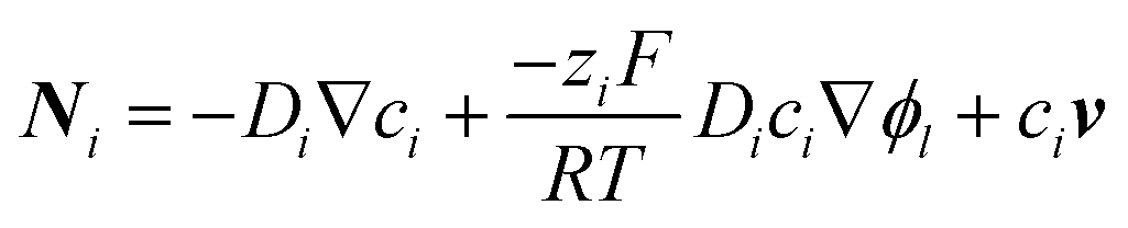 | (1) |
In the literature, two types of devices are often studied to simulate the above-mentioned effects: a flow cell and a stagnant cell. In flow cells, well-defined convection conditions, such as laminar flow, are typically established, which help to provide fresh bulk electrolyte to the electrode surface.31,48–50 Hydrodynamic control in such a cell is required to mitigate mass-transport limitations. The influence of the flow rate on the local pH gradient has been evaluated in flow cells.31,48 However, the situation is much less defined in a stagnant cell, which is typically used for (photo)electrochemical measurements. To simulate a stagnant cell, a boundary layer with an arbitrary thickness of 0.1–2 mm is often assumed to be present.51,52 In this assumption, diffusive and migrative mass transport of dissolved species occur only within the boundary layer while their concentrations are assumed to be constant outside the boundary layer. Concentration gradients, therefore, appear only within the boundary layer, and the concentration overpotential strongly depends on the more or less arbitrarily chosen thickness of the boundary layer.51 Also, electrolyte convection is often overlooked, even though electrochemical reactions in realistic electrochemical cells generate natural convection due to the formation of product gas bubbles and/or buoyancy effects as a result of changes in local electrolyte density.53–60
In this work, we combine in situ measurements and computational modeling to visualize and validate the pH distribution in an electrochemical cell. The local pH is quantitatively monitored using fluorescence pH sensor foils during water splitting in stagnant and pH-neutral solutions. Our experimental setup allows a quick assessment of pH gradients not only at regions close to the electrodes but also throughout the entire electrochemical cell. Based on the observed pH gradients, we develop an advanced multiphysics model coupled with natural convection induced by buoyancy effects during electrochemical reactions. We will show that the model can describe how the local pH stabilizes in stagnant conditions and underlines the significant contribution from the natural convection. Finally, the implications of our findings for the design of efficient energy conversion devices in the presence of natural convection are discussed.
Results and discussion
1. In situ pH monitoring during electrochemical water splitting in near-neutral pH solutions
We first monitor the local pH change (ΔpH) of electrolytes during water splitting in a simple two-electrode electrochemical cell by camera imaging of a fluorescence pH sensor foil. The foil is immersed between a vertically aligned Pt anode and Pt cathode, as shown schematically in Fig. 1a. Two types of foils were used: one with a pH detection range from 5 to 8, and another from 6 to 8.5; see Fig. S1a (ESI†) for the calibration curves of the foils. The operating principle of the pH sensor foil is briefly described in the Experimental section. Digital photographs of the electrochemical cell are shown in Fig. S1c and d (ESI†). Fig. 1b shows ΔpH during electrochemical water splitting in 0.5 M K2SO4 (pH = 7) at 1 mA cm−2 (see also Movie S1, ESI†). It can be clearly seen that the local pH shifts to more acidic and alkaline values in the regions close to the anode and cathode, respectively. In neutral pH solutions, since the concentration of protons and hydroxide ions are low, the water reduction and oxidation reactions can be expressed as follows:| 4H2O + 4e− → 2H2 + 4OH− | (2) |
| 2H2O → O2 + 4H+ + 4e− | (3) |
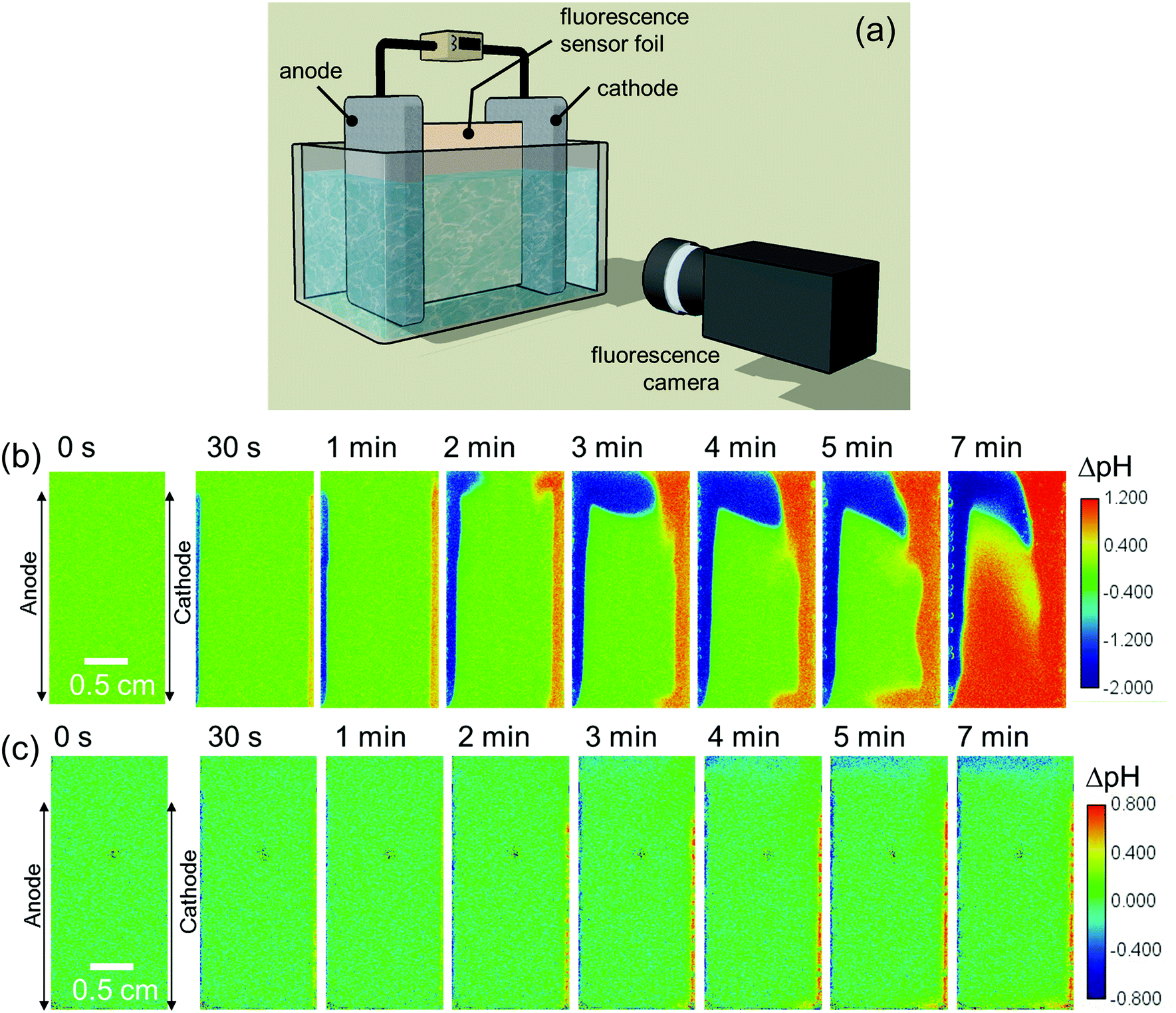 | ||
| Fig. 1 (a) Schematic of our in situ fluorescence pH monitoring setup, used to measure the pH distribution in an electrochemical cell during water splitting. The distribution of local pH change (ΔpH) is shown at 1 mA cm−2 in (b) 0.5 M K2SO4 and (c) 0.1 M KPi. The initial pH of both electrolyte solutions is 7. | ||
The effect of a pH buffer on the ΔpH is examined by replacing the electrolyte with a 0.1 M potassium phosphate (KPi) buffer solution. Phosphate ions are thermodynamically stable inorganic buffer species during electrochemical water splitting reactions.61 In this case, the ΔpH is observed mainly in the close vicinity of electrodes (within 1 mm) during a chronopotentiometric experiment at 1 mA cm−2 (Fig. 1c and Movie S2, ESI†). Slightly acidic and alkaline regions are also observed at the top and bottom of the cell, respectively, which will be discussed later, but the electrolyte's pH in the middle of the cell does not change. The present observation, therefore, confirms that buffer ions work as proton/hydroxide donors that stabilize the pH during water splitting. The reactions that are responsible for the pH buffering are given by
| HA ⇆ H+ + A− | (4) |
| A− + H2O ⇆ OH− + HA | (5) |
Although the observed pH changes (both in unbuffered and buffered electrolytes) are not surprising and commonly known to occur for pH-neutral solutions, we note that—to the best of our knowledge—this is the first direct spatially-resolved visualization experiment of local pH changes in a complete electrochemical water splitting cell. We also emphasize that while Pt electrodes are used here as the anode and cathode, the observed pH changes are independent of the electrode materials for a given set of reaction conditions, i.e., current density, electrolyte and cell configuration.
For a better comparison, the observed pH shifts (averaged over the vertical direction) are plotted against the horizontal direction from the anode to the cathode. The ΔpH profiles continuously change in 0.5 M K2SO4 during 10 mins of the experiment (Fig. S2a, ESI†), but in phosphate buffer solutions they stabilize after ∼3 min of electrolysis (Fig. S2b, ESI†). This stabilization also occurs when the current density is increased from 1 mA cm−2 to 10 mA cm−2 (Fig. S2c, ESI†). In the unbuffered 0.5 M K2SO4, the pH in the middle of the cell changes significantly at higher current densities (Fig. 2a), and the plateau regions close to the electrodes indicate that the pH shifts beyond the detection range of the fluorescence foil. In contrast, all the measured pH values in the phosphate buffer solutions are well within the detection range (Fig. 2b and c). In 0.1 M KPi solution, the applied current density has a large impact on the pH close to the electrodes, especially at the cathode side. The ΔpH close to the cathode largely increases from 0.5 to 1 when the applied current density is increased from 1 to 2 mA cm−2 (Fig. 2b). This indicates that the local concentration changes exceed the buffer capacity. Above 5 mA cm−2, the alkaline region further expands towards the middle of the cell (see Fig. 2b and Fig. S3, ESI†). The pH shift can be further suppressed by increasing the buffer concentration to 0.5 M (Fig. 2c); even at a current density of 10 mA cm−2, the pH change is limited to less than 0.5 units.
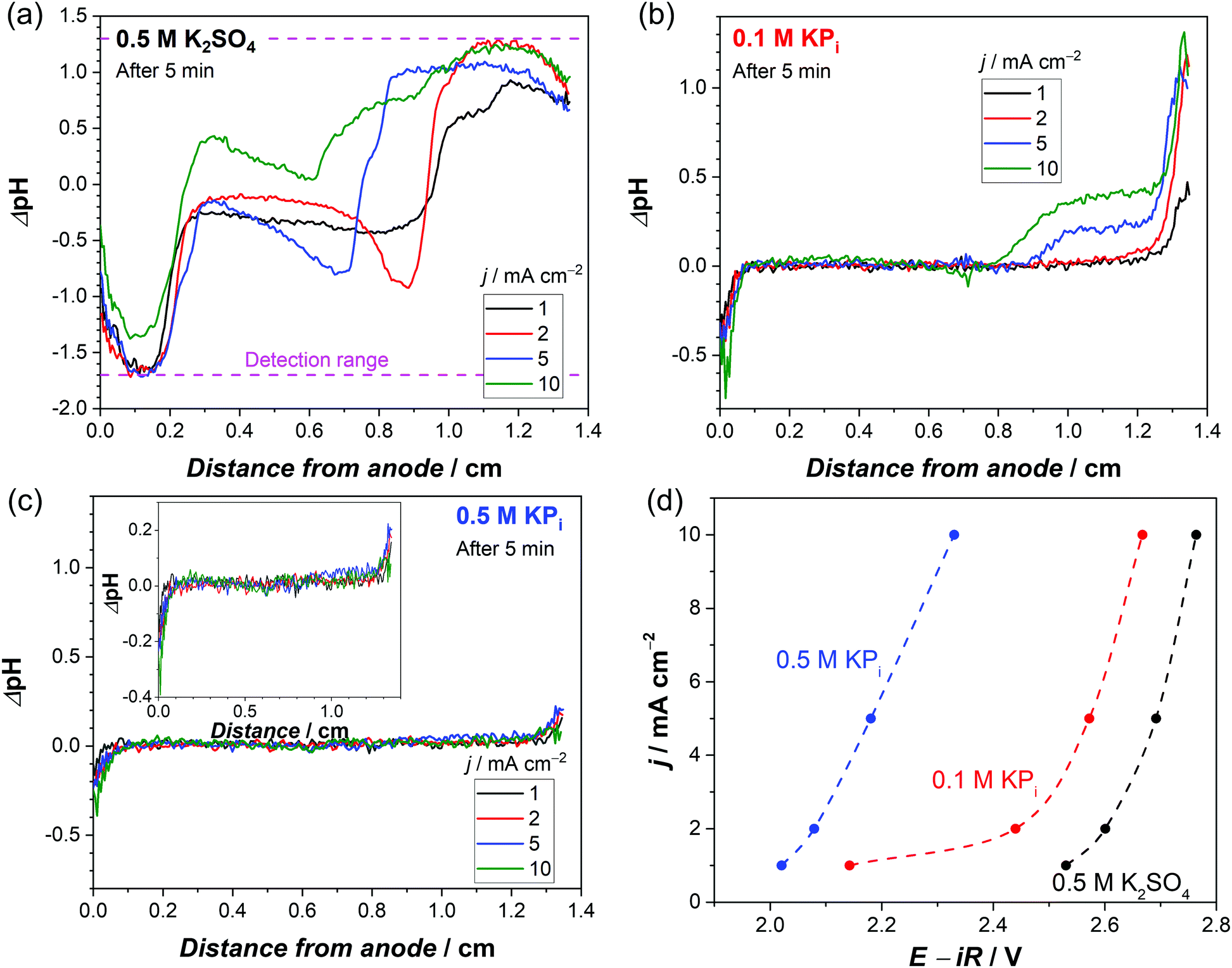 | ||
| Fig. 2 Average ΔpH profile from the anode to the cathode after 5 min of chronopotentiometry at different current densities in (a) 0.5 M K2SO4, (b) 0.1 M KPi and (c) 0.5 M KPi. Both the anode and cathode are Pt/Ti/FTO electrodes. (d) Current–voltage response obtained from the stabilized chronopotentiometry data (after 10 min) using Pt/Ti/FTO electrodes in 0.5 M K2SO4, 0.1 M KPi and 0.5 M KPi (non-stirred condition, room temperature). The voltages are corrected for iR drop, see Fig. S4 (ESI†) for specific R values of the different electrolytes. The dashed lines are guides to the eye. | ||
Fig. 2d shows the steady-state iR-corrected current–voltage response of the electrochemical cell; the datapoints were obtained from the plateaus of the chronopotentiometry measurements shown in Fig. S4 (ESI†). These curves clearly show that adding a supporting buffer effectively suppresses the overpotential. Notably, the required voltage in 0.1 M KPi solution sharply increases (by ∼300 mV) when the current density is increased from 1 to 2 mA cm−2. This is consistent with the observed jump of ΔpH at the cathode side (Fig. 2b); the local pH shifts far from the pKa2 (= 6.8) due to mass transport limitation of phosphate ions close to the cathode. Such a sharp increase in voltage is not observed in the 0.5 M KPi solution. Instead, the voltage monotonically increases with increasing current density, in agreement with the fact that no significant pH shift was observed with increasing current density (Fig. 2c).
A closer look at the pH distribution measured at 1 mA cm−2 in an unbuffered solution (Fig. 1b) reveals the presence of natural convection. The images show that the acidic and alkaline regions move upward and downward, respectively, resulting in a clockwise circulation. A similar flow pattern was also observed by particle image velocimetry (PIV) during water splitting with vertically aligned electrodes in KOH at ca. 0.2 mA cm−2.55
To confirm that the observed natural convection is purely driven by the electrochemical reactions and not some artefact of the setup, we switched the anode and cathode sides by reversing the polarity. As expected, the pH distribution appears as a mirror image of the original one (Fig. S5, ESI†vs.Fig. 1b). The flow pattern becomes different when the current density is above 5 mA cm−2; both the acidic and alkaline regions move upward (Fig. S6, ESI†). Under these conditions, the contribution from rising gas bubbles, which drag the surrounding electrolyte along, becomes dominant. This clearly indicates bubble-induced convection, which was also previously reported during bubble velocity measurements at current density >3 mA cm−2.62 This is also consistent with the presence of the plateau region growing from the cathode side above 5 mA cm−2 (see Fig. 2a and b, and pH distribution in Fig. S3 and S6, ESI†), which is caused by the fact that more gas bubbles are produced at the cathode than at the anode (i.e., two H2 for every O2).
The electrolyte velocity in the horizontal direction at the top and bottom of the electrochemical cell can be estimated from a series of snapshots of the observed pH distribution. Fig. 3 shows that the electrolyte velocity increases as the current density increases, as would be expected. Although the horizontal velocity is most pronounced in the unbuffered electrolyte, a similar convection pattern also seems to form in the buffered electrolyte. This is evident from the pH distribution in 0.1 M KPi at 1 mA cm−2: slightly acidic and alkaline regions are observed at the top and bottom of the cell, respectively (Fig. 1c).
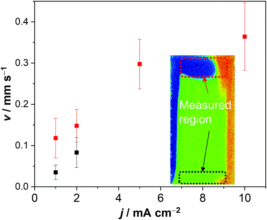 | ||
| Fig. 3 Velocity measured from the pH distribution in 0.5 M K2SO4, by tracking the pH change in the horizontal direction at the top (red) and bottom (black) of the cell (see inset for the measured region). | ||
In the next section, the origin of the observed natural convection at low current densities (∼1 mA cm−2) and its impact on the local pH distribution in the cell are further studied and validated with multiphysics simulations.
2. Multiphysics simulation during electrochemical water splitting with buoyancy effects
We first discuss what physical effects could cause the observed clock-wise convection. At low current densities, bubble-induced convection is negligible and the convection is likely caused by changes in the electrolyte density. Two possible factors modify the local electrolyte density during water splitting: (i) dissolved product gases and (ii) change of ion concentration. Although changes in the electrolyte density due to dissolved gases are rarely reported, the magnitude of this effect can be predicted from the expansion coefficient, α,63 according to the following equation: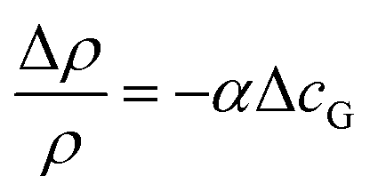 | (6) |
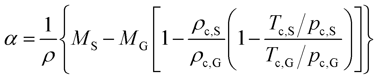 | (7) |
An alternative explanation for a change in the local electrolyte density is a change in the nature and concentration of ions. For example, during Fe(CN)64−/3− redox reactions in non-stirred electrolytes, it has been reported that the electrolyte close to the cathode becomes heavier because of the increasing concentration of reduced Fe(CN)64− species followed by increased cation concentration, and vice versa for the electrolyte close to the anode (note that the masses of these redox ions are the same, so in this case, it is the oxidation state of the ion and the resultant cation concentration that affects the density of the solution).53,54 During proton-coupled electron transfer reactions, the local pH at the cathode side becomes more alkaline. In a phosphate buffer solution, this is compensated by the increase of dibasic (K2HPO4) or tribasic phosphate (K3PO4) concentration. Since K2HPO4 and K3PO4 have a higher density than the bulk 0.1 M phosphate buffer (see Fig. S7a, ESI†),64,65 the electrolyte close to the cathode becomes heavier. The opposite is true for the electrolyte close to the anode, i.e., the KH2PO4 and/or H3PO4 concentrations increase while buffering the protons that are being produced, and the electrolyte density decreases. In other words, the electrolyte close to the anode would move upward, and the electrolyte close to the cathode would move downward. This is very much in agreement with our observed electrolyte circulation and a likely explanation for the observed natural convection.
To confirm the above-mentioned explanation, a two-dimensional model combining fluid dynamics and electrochemistry was developed which takes into account the local electrolyte density dependence on the local ion concentrations. The following mass-transport equation was used to describe the local ion concentrations:
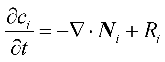 | (8) |
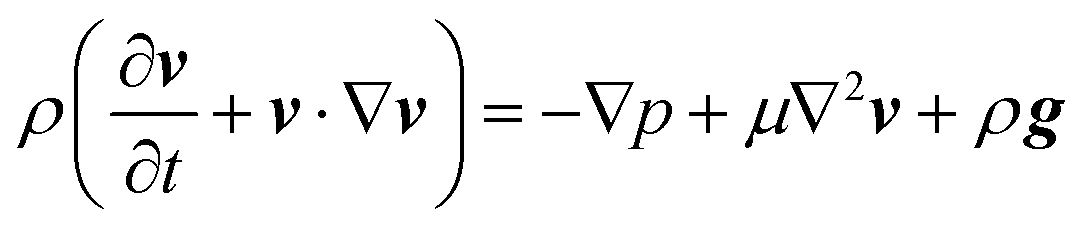 | (9) |
 | (10) |
We note that a change in local electrolyte density can also be induced by local temperature changes due to the overpotentials at the electrodes. However, even at 400 mV of overpotential and a current density of 100 mA cm−2 (i.e., 10–100× higher than the current densities used in our study), the dissipated power of 40 mW cm−2 leads to a temperature increase of less than 0.1 °C in 10 seconds, which is negligible. Isothermal conditions are therefore assumed in our simulation.
Fig. 4a shows the simulated local electrolyte density in 0.1 M KPi at 1 mA cm−2. The electrolyte becomes heavier and lighter close to the cathode and anode, respectively, during water splitting due to the migration of potassium ions. Close to the electrodes, the local electrolyte density changes by 0.1% compared to the density of the bulk solution. Although the 0.1% change in the local electrolyte density is very subtle, it is sufficient to generate natural convection driven by buoyancy effects. Fig. 4b shows the simulated velocity field in 0.1 M KPi at 1 mA cm−2, with the velocity vectors indicated by the arrows. The direction of the simulated velocity closely resembles the observed natural convection (Fig. 1b and c), in which the electrolyte close to the anode and the cathode moves upward and downward, respectively. The simulated velocity profile starts to stabilize after 100 seconds. At the top and bottom of the electrochemical cell, the horizontal velocity is approximately 0.05–0.1 mm s−1, which is in excellent agreement with the velocity obtained from in situ pH measurements in 0.5 M K2SO4 shown in Fig. 3. We note that the simulated velocity close to the electrode surfaces (<1 mm) is even higher, reaching 0.35 mm s−1. This is consistent with the idea that the driving force for the natural convection is the change of the local ion concentrations during electrochemical reactions at each electrode.
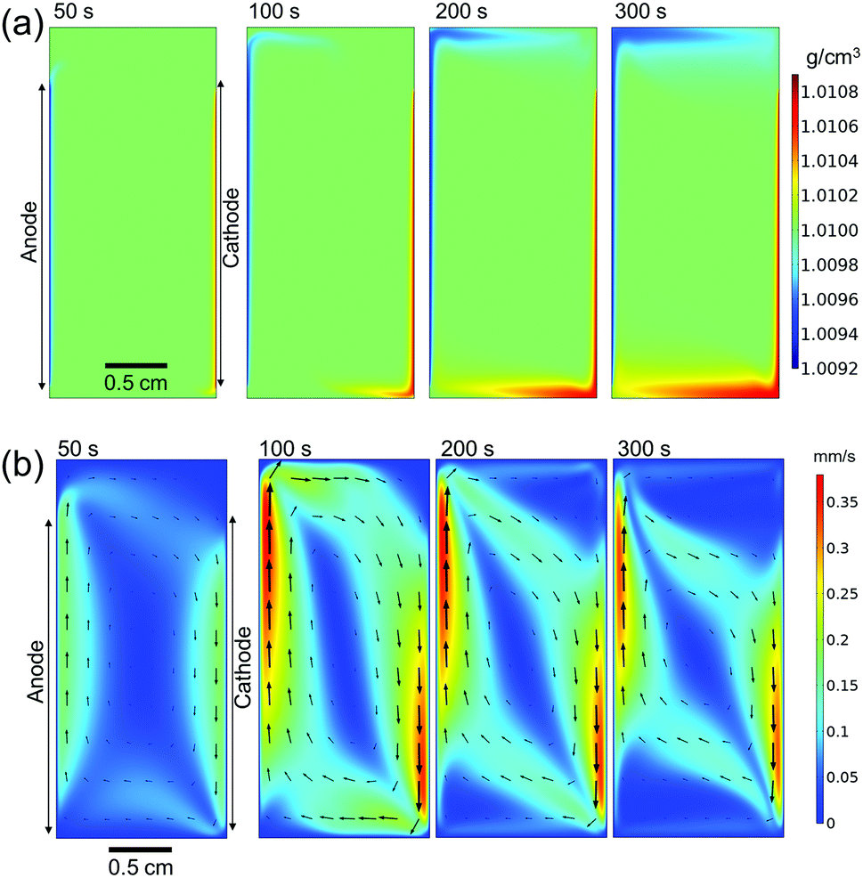 | ||
| Fig. 4 (a) Simulated electrolyte density profile and (b) simulated velocity in 0.1 M KPi solution at 1 mA cm−2. Arrows in (b) represent the velocity vectors. Simulations are performed with buoyancy effect. | ||
We now turn our attention to the influence of buoyancy-driven natural convection on the pH gradient. Fig. 5a shows the simulated pH at the center of the electrode surface (1.2 cm from the bottom of the cell) during electrochemical water splitting in a 0.1 M KPi solution at 1 mA cm−2, with and without buoyancy effects. In the absence of buoyancy effects, the electrolyte density is assumed to be constant and the velocity in the cell is zero (i.e., no convection of the liquid, only diffusion, and migration of ions). As a result, the local pH continuously changes both on the anode and cathode. After ∼100 s, the pH starts to rapidly change, and after ∼180 s convergence can no longer be obtained. The rapid change happens because the supporting buffer cannot suppress pH shifts effectively at pH levels far from pKa2 = 6.8 at the given buffer concentration.51,66,67 In the presence of buoyancy effects, the simulated pH initially follows the one without buoyancy effects for t ≤ 50 s; at this stage, natural convection has not yet fully developed (see Fig. 4b). After ∼180 s, the local pH starts to stabilize both on the anode and the cathode. The simulation indicates that fresh bulk electrolyte with additional proton/hydroxide donors is provided to the electrodes by convective mass-transport. The simulated stabilization process agrees with our observation during in situ pH monitoring, in which a stabilized pH profile was obtained after 3 minutes of electrolysis (Fig. 1c and Fig. S2b, ESI†).
 | ||
| Fig. 5 (a) Simulated pH at the electrode surface as a function of time in 0.1 M KPi at 1 mA cm−2 with and without buoyancy effect. Comparison of simulated and measured ΔpH profile in 0.1 M KPi after chronopotentiometry for 120 and 180 seconds at 1 mA cm−2 close to (b) anode and (c) cathode. Insets show a larger magnification of regions close to the electrodes. | ||
The simulated and measured pH profiles are compared in Fig. 5b and c for electrolytes close to the anode and cathode, respectively. When the buoyancy effect is ignored, large pH shifts up to 3 pH units are predicted within 300 μm from both electrodes. This clearly does not agree with the experimental data; it can, therefore, be concluded that a simple diffusion–migration model overestimates the pH gradient under stagnant conditions. On the other hand, our diffusion–migration–convection model coupled with the buoyancy effect can reproduce the measured pH profile close to the electrodes with reasonable accuracy. Although the resolution of our pH sensor foil (100 μm) limits us from capturing the local pH directly at the electrode surface, our results clearly show that a pH shift of ca. 1 unit (at both electrodes) develops even at low current densities (1 mA cm−2) in a stagnant 0.1 M KPi solution. Although the corresponding concentration overpotential of ∼120 mV is still significant, it is substantially less than the overpotentials that would develop without buoyancy effects.
It has been recently shown that pH shifts are expected to be amplified when scaling-up electrode sizes.17,31 To highlight the impact from scaling-up, the sizes of all the geometric parameters in our model were doubled while maintaining the electrolyte solution and the applied average current density. The pH shifts are indeed found to increase with device size (Fig. S10a, ESI†). The buoyancy-driven convection velocity is higher in the larger device due to the higher total current (Fig. S10b, ESI†), but it is insufficient to compensate the build-up of local pH shift along the electrodes (Fig. S10c, ESI†).
We note that the presence of the fluorescence foil may influence the hydrodynamics in the electrochemical cell. Since the existence of the foil is not considered in our model, the simulated velocity may be overestimated, since the foil will exert some drag on the electrolyte solution. This would result in an underestimation of the pH shift. Rigorously speaking, three-dimensional simulations are required to fully evaluate the transport phenomena close to the foil and the electrodes. Alternatively, in order to obtain 2D map of fluorescence signals without any interference from the foil, one could dissolve fluorescent dyes in the electrolyte and excite these in a 2D plane by a sheet-shape laser source.55 Nevertheless, considering the good agreement between our measurements and numerical simulations, the influence of the foil on the convection profile seems small and is unlikely to affect our main conclusions.
3. The implication of buoyancy-driven natural convection to the design of (photo)electrochemical energy conversion devices
We now consider the implication of our findings on the design of (photo)electrochemical water splitting devices. First, despite the positive influence in reducing local pH shifts, natural convection may promote product gas crossover between the anode and cathode in membrane-free water-splitting devices. Fig. 6a–c shows the simulated O2 concentration in a closed batch reactor at 1 mA cm−2. Here, O2 is assumed to remain dissolved in the (supersaturated) electrolyte solution (i.e., bubble formation is ignored in this simulation). O2 remains close to the electrode surface in the absence of natural convection (Fig. 6a) because the crossover of O2 solely relies on diffusive mass-transport. When the buoyancy effect is taken into account, dissolved O2 follows the simulated flow pattern shown in Fig. 4 and reaches the cathode surface via the top of the electrochemical cell (Fig. 6b and c). To experimentally validate this simulation, the concentration of dissolved O2 was monitored with an O2 sensitive fluorescence foil after complete degassing by N2 bubbling (Fig. 6d, e, and Movie S3, ESI†). The measured concentration is approximately 10 times smaller than the simulated one. This is because bubble formation is ignored in the simulation; part of the generated O2 bubbles can be observed in the measured images. Nevertheless, the measured patterns of the concentration gradient are well reproduced by the simulated ones that include buoyancy effects, which further validates our mass transport model coupled with buoyancy-driven convection. Any O2 that crosses over to the cathode side decreases the purity of H2—the produced H2 at the cathode surface already contains 2 mol% of O2 after 300 s of electrolysis—and presents a potential safety hazard by forming an explosive gas mixture. Besides, the O2 that crosses over can be reduced at the cathode, which is an undesired side-reaction resulting in the loss of faradaic efficiency for H2 formation.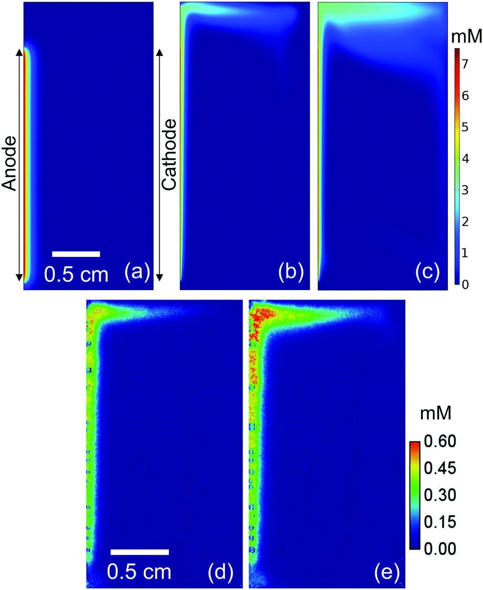 | ||
| Fig. 6 (a) Simulated O2 concentration distribution without buoyancy effect at t = 150 s. The same simulation results but with the consideration of buoyancy effect are shown in (b) at t = 150 s and (c) at t = 300 s. The simulation is validated by directly measuring the O2 concentration using an O2 sensitive fluorescence film (d) at t = 150 s and (e) at t = 300 s. In all cases, the electrolyte is 0.1 M KPi and the current density is 1 mA cm−2. | ||
Mitigating approaches, for instance by using an ion-exchange membrane between the anode and cathode, are therefore required to utilize the natural convection effectively in a stagnant electrochemical cell. Alternatively, the laminar flow may be introduced to improve mass-transport and product gas separation in membrane-free devices, as demonstrated in a few reports in the literature.31,48–50,68–71 Stirring the electrolyte (i.e., with a stir bar) is also a simple and common approach to improve mass-transport, but would promote undesired product cross-over. Moreover, it is not trivial to quantitatively describe the velocity profile, as it is highly dependent on the location of the electrodes, the stir bar, the 3-D shape of the cell, etc. We therefore compare the velocity profile of natural convection driven by electrochemical reactions (at 1 mA cm−2) to that of forced laminar flow in Fig. 7. While natural convection develops in close vicinity of the electrodes (<1 mm), the maximum velocity for forced laminar flow appears far away from the electrodes in the middle of the channel. Since the pH gradient appears within 1 mm from the electrodes, convection in this region is critical to replenish the supply of proton/hydroxide donors. To obtain a velocity close to the electrode comparable with the natural convection, an average inlet velocity of 2–3 mm s−1 would be required for the cell with forced laminar flow (see Fig. 7b). In other words, to minimize the contribution from natural convection in laminar flow devices, the average inlet velocity needs to exceed the natural buoyancy-induced convection velocity by one or two order of magnitudes.
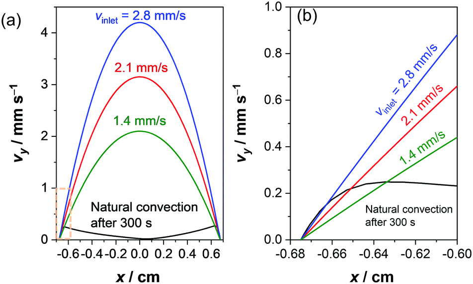 | ||
| Fig. 7 (a) Comparison of the velocity profile between the simulated natural convection and laminar flow. The average inlet velocities in a laminar flow cell were chosen to obtain a velocity close to the electrode similar to the natural convection. The velocity for the natural convection is taken after applying 1 mA cm−2 for a period of 300 seconds, at which the velocity profile has been stabilized. (b) Magnification of the velocity profile close to the electrode. | ||
Based on our multiphysics model, we also investigate the buoyancy-driven natural convection and its effect on local pH shifts in other buffer solutions: sodium phosphate (NaPi) and potassium carbonate (KCi). These buffer solutions are also often applied for (photo)electrochemical water splitting in near-neutral pH conditions. The respective electrolyte density functions (Fig. S7b and c, ESI†) and diffusion coefficients (Table S1, ESI†) are introduced in the model accordingly. Fig. 8a shows the simulated pH at the center of the electrodes for the different buffer solutions. At t < 100 s, the local pH change (ΔpH) in KPi and NaPi overlaps each other, while the ΔpH in KCi is smaller. During this time, natural convection is not yet fully developed (see Fig. 4b). ΔpH is therefore mainly determined by the diffusive mass-transport of buffer anions to counter proton or hydroxyl ion accumulation.23,29,30 Indeed, the diffusion coefficients of carbonate anions are higher than those of phosphate anions (see Table S1, ESI†). At t > 100 s, natural convection begins to stabilize (see Fig. 4b) and influence the ΔpH, which is why the ΔpH starts to differ between NaPi and KPi. At the end (t = 300 s), the ΔpH is the largest in NaPi and the smallest in KCi. This trend agrees very well with the trend of the natural convection velocity, as shown in Fig. 8b. The velocity at 400 μm away from the anode—where the maximum velocity is observed (see Fig. 7b)—is shown. Higher velocities due to natural convection further suppress the local pH shifts close to the electrodes. We note that the same correlation is also observed at the cathode side (not shown).
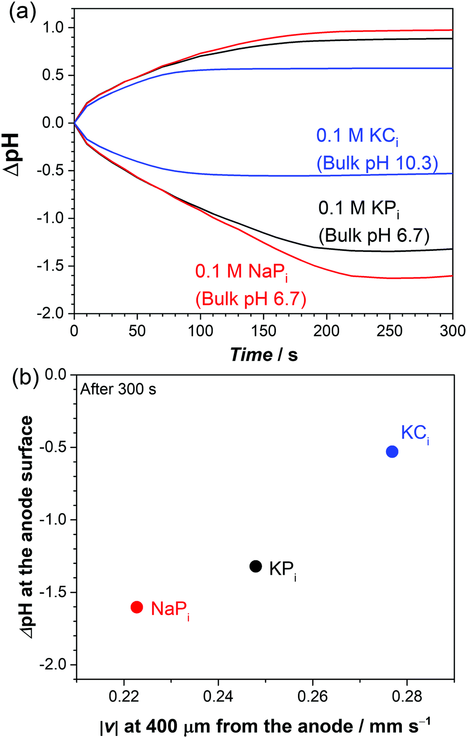 | ||
| Fig. 8 (a) Simulated pH change as a function of time in 0.1 M KPi, NaPi, and KCi at 1 mA cm−2. (b) Simulated local ΔpH at the anode surface vs. velocity after 300 s with varying electrolytes. | ||
Despite the good agreement between the ΔpH and the velocity in Fig. 8b, the velocity trend cannot be fully explained by the density of the buffer solutions. Based on the density functions (Fig. S7, ESI†), for a given concentration, the density of KCi < NaPi < KPi. One would therefore initially expect the velocity in KCi > NaPi > KPi. This is not what we observed in Fig. 8b; the velocity in KCi is indeed the highest, but the velocity in NaPi is instead smaller than that in KPi. This suggests that factors other than the density functions also play a role in determining the natural convection velocity.
We, therefore, examine the influence of the diffusion coefficients of both cations and anions to the change of local electrolyte density, which would in turn affect the natural convection velocity. Additional simulations were performed where the diffusion coefficients of KPi are modified (Fig. S11, ESI†); either the diffusion coefficient of the cation (Dcation) is changed to that of sodium or the diffusion coefficients of anions (Danion) are changed to those of carbonate ions. Again, only regions close to the anode are shown, but the same effects are observed for regions close to the cathode. The main effect of the change in the diffusion coefficient lies in the additional accumulation of anions close to the surface of the anode (see Fig. S11a, ESI†). When Dcation is decreased to the value of sodium, the increased accumulation of anions largely decreases the local density change (Δρ, see Fig. S11b, ESI†). The smaller Δρ suppresses the buoyancy effect, and this, therefore, explains our observation that the velocity in NaPi is smaller than that in KPi. When Danion is increased to the value for carbonates, an increased accumulation of anions is also observed but it decreases Δρ to a much smaller extent. This contributes to the suppression of the buoyancy effect, but it is not enough to compensate for the generally lower density of KCivs. KPi. As a result, the velocity in KCi is still higher than that in KPi.
We acknowledge that part of the effect observed when comparing KPi and KCi also comes from the difference of the bulk pH (i.e., 6.7 vs. 10.3). This effect is, however, relatively minor as compared to the influence of the density and diffusion coefficient. Only ∼14% of the suppression of ΔpH is contributed by the bulk pH (see Fig. S12, ESI†). Overall, the delicate balance between the diffusion coefficient of ions and the density of the electrolyte determines the natural convection and the resulting local pH gradients.
The influence of buoyancy-driven convection to the pH shift is also evaluated in highly alkaline electrolytes. We did this for a 0.1 M KOH solution (pH 13, the electrolyte density is shown in Fig. S7d, ESI†) at a current density of 1 mA cm−2. The simulated pH shift, shown in Fig. S13 (ESI†), is negligible compared to that in buffered neutral pH solutions (Fig. 8a), even without considering buoyancy effects. This agrees with the often-made assumption that mass-transport does not play a significant role at sufficiently high pH values, due to the abundance of highly mobile hydroxide ions in the bulk solution. Although buoyancy-driven convection still helps to stabilize the pH shift in highly alkaline conditions, it may be difficult to observe its contribution during electrochemical measurements.
We point out that our quantitative discussions are limited to low current densities (<2 mA cm−2). Under these conditions, bubble formation does not contribute to the convection of the electrolyte, as shown in a recent report on gas evolving electrodes.62 It should be realized, however, there are many aqueous electrochemical reactions in which bubble formation does not play a role. For such reactions, our buoyancy-driven convection model may offer useful insights for current densities well beyond 2 mA cm−2. Examples of such reactions are oxidative upgrading of biomass feedstocks and production of oxidizing agents like hydrogen peroxide and peroxydisulfate anions.72–77 On the cathode side, formate and alcohol production from CO2 and ammonia synthesis from N2 have been extensively studied.78,79 The (photo)electrochemical reduction of nicotinamide adenine dinucleotide (NAD+) results in a versatile reducing agent that can be used for a wide range of biocatalytic redox reactions to produce valuable chemicals.80,81 All of these reactions involve proton coupled electron transfer reactions without forming product gas bubbles, and in all these cases it is desirable to minimize pH shifts during reactions. In order to shed light on the potential impact of buoyancy-driven convection for such reactions at current densities beyond 2 mA cm−2, additional calculations were performed. A higher buffer concentration (1 M vs. 0.1 M KPi) was chosen to prevent a total depletion of ions at higher current densities. As expected, the pH shifts are more severe at higher current densities (Fig. 9a), and the increase in the buoyancy-driven convection velocity with current density (Fig. 9b) is insufficient to completely prevent the pH shifts. Notably, the pH shifts never stabilize for any of the current densities in the absence of the buoyancy effects, which clearly demonstrates the significance of natural (i.e., buoyancy-driven) convection even at high current densities. We note that additional buoyancy effects may be present due to the production of aqueous products. Moreover, additional concentration overpotentials from the additional reactants (e.g., CO2 or N2) need to be considered, but these are beyond the scope of this study.
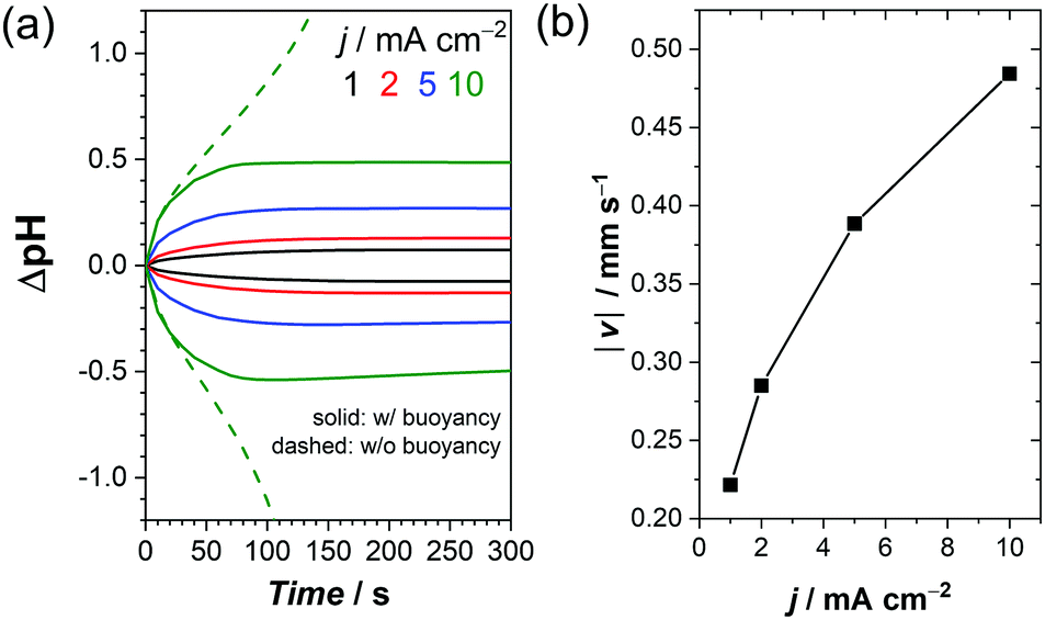 | ||
| Fig. 9 (a) Simulated pH change at the electrode surfaces as a function of time at different current densities in 1 M KPi. (b) Simulated maximum buoyancy-driven velocity close to the anode at different current densities after 300 s in 1 M KPi. | ||
Fig. 9b also shows that our simulated buoyancy-driven velocity close to the electrode reaches ∼0.5 mm s−1 at 10 mA cm−2. This is smaller, but not negligible, compared to the reported bubble velocity of 4–5 mm s−1 at this current density.62 In other words, buoyancy-driven convection is likely to affect the overall electrolyte dynamics and the resulting pH gradient. It therefore has to be taken into consideration in solar water splitting, even at higher current densities.
Conclusions
In this study, local pH changes during electrochemical water splitting in neutral pH solutions were detected using an in situ fluorescence pH monitoring setup. By comparing the pH distribution in buffered vs. unbuffered electrolytes, the presence of supporting buffer ions was shown to minimize and limit local pH shifts to regions close to the electrode surfaces (<1 mm). We also showed that natural convection occurs in stagnant conditions, an effect which has been ignored in previous studies on PEC cells. To simulate these effects, a two-dimensional multiphysics model was developed by combining electrochemistry and computational fluid dynamics coupled with buoyancy effects due to the change of electrolyte density, which play a role especially at lower current densities (<2 mA cm−2). The model successfully reproduced the observed electrolyte convection and pH shifts driven by electrochemical reactions. This advanced validated model clearly demonstrates that buoyancy-driven natural convection helps to stabilize the pH and reduce overpotentials. Our study also revealed that the types of ions in the buffer solutions (e.g., potassium vs. sodium, phosphate vs. carbonate) significantly affect the buoyancy-driven convection, which is something that should be taken into account when motivating the choice of electrolyte solutions in a water-splitting device. Finally, buoyancy-driven natural convection can also play an important role in electrochemical reactions without any gaseous products. For such reactions, the absence of bubble-induced convection means that buoyancy effects may dominate the total convection also at higher current densities.Experimental
Electrochemical measurements
200 nm of Pt was evaporated on the FTO substrate with 5 nm Ti as an adhesion layer. Depositions were done by electron beam evaporation (Telemark) in a customized high vacuum deposition chamber pumped by a typical dry turbo molecular pumping set with a typical base pressure of 2 × 10⁻⁷ mbar. Deposition rates of 0.15 nm s−1 for Ti (0.4 kW e-beam power) and 0.65 nm s−1 for Pt (2 kW) were used and controlled during deposition using a quartz crystal microbalance. Part of the Pt surface was connected to an electrical wire with a conductive tape, which was afterwards insulated using an epoxy resin. The Pt/Ti/FTO electrodes were used as the anode and the cathode with an active area of 5 cm2. Potassium phosphate (KPi) buffer solutions were prepared from KH2PO4 (Sigma-Aldrich, ≥99.0%) and K2HPO4·3H2O (Sigma-Aldrich, ≥99.0%) to obtain the desired pH. Potassium sulfate unbuffered solution was prepared by dissolving K2SO4 (Sigma-Aldrich, ≥99.0%) in water without any pH adjustment. The water used in all experiments was obtained from a Milli-Q Integral system with a resistivity of 18.2 MΩ cm.All the electrochemical measurements were performed under a two-electrode configuration using a VersaSTAT 3 potentiostat/galvanostat (AMETEK). Uncompensated resistance (Ru) was obtained from impedance measurements, and iRu corrections were performed to the applied voltage unless otherwise stated. The distance between the anode and cathode was 1.4 cm.
Fluorescence signals from pH sensor foils (SF-HP5R and SF-HP51R, PreSens) and O2 sensor foils (SF-RPSu4, PreSens) immersed perpendicularly between the anode and cathode were detected by VisiSens™ TD Basic System (PreSens). The pH sensor foils incorporate green fluorescent pH indicator dyes and inert red fluorescent dyes as references. The luminophores are excited by the blue LEDs incorporated in the camera. The ratio between the green and red fluorescent signals, which are collected through the wavelength-separated red and green channels in the RGB camera detector, are used for the calibrations and the measurements. The calibration of pH sensor foils was performed in 0.1 and 0.5 M KPi solutions with different pH (Fig. S1a, ESI†). O2 sensor foils were calibrated in 0.1 M KPi with N2 bubbling (Air Liquide, purity ≥99.999%, O2 impurity ≤2 ppm), and ambient air saturation (Fig. S1b, ESI†). The solubility of O2 in 0.1 M KPi solution was reported to be 1.2 mM.29
Computational modelling
Time-dependent simulations were performed by solving the governing conservation and transport equations (see Results and discussion section) with COMSOL Multiphysics®. All the parameters used, the schematics of multiphysics modeling and the optimized mesh was shown in Table S1, Fig. S8 and S9 (ESI†), respectively. Additional details on the simulations are described in Supplementary Note 1 (ESI†). Relative tolerance of 0.001 was applied as the convergence criterion. To simulate the transport of chemical species, the theory of diluted species, which ignores an interaction between ions, was applied. Charge neutral (∑zici = 0) and equilibrium of buffer species was assumed in our model. No flux boundary (n·Ni = 0) and insulating boundary (n·F∑ziNi = 0) conditions were applied for all the cell walls and the top of the electrolyte except for the electrodes. At the electrode surface, a stoichiometric amount of proton, hydrogen and oxygen were either produced or consumed, assuming 100% faradaic conversion efficiency. Bubble formation is ignored and the product gases were assumed to be supersaturated in the electrolyte solutions. The electric potential (ϕs) of the cathode was set to be zero. Butler–Volmer equation was used on the electrodes to determine the electrode potentials at each set of current density. Since the resistivity of Pt electrodes used in our experiments is very small, the resistance through the electrode in our simulation was ignored; the potentials were therefore constant within the electrodes. Local electrolyte density was determined by local ion concentrations using the reported values shown in Fig. S7 (ESI†), assuming a linear relationship with the concentration of cations and anions.To model the convection within the cell, the laminar flow was assumed. All the walls were assumed to be no slip (v = 0). From the kinematic viscosity, characteristic length, and maximum velocity simulated, the Reynolds number was determined to be 3. Since the simulated Reynolds number is <2000, the laminar flow assumption is validated.
Conflicts of interest
There are no conflicts to declare.Acknowledgements
All authors acknowledge support from the Deutsche Forschungsgemeinschaft (DFG, German Research Foundation) under Germany's Excellence Strategy – EXC 2008/1 (UniSysCat) – 390540038 and from the German Helmholtz Association – Excellence Network – ExNet-0024-Phase2-3. This work was carried out with the support of the Helmholtz Energy Materials Foundry (HEMF), a large-scale distributed research infrastructure founded by the German Helmholtz Association. The authors also acknowledge Dr Ibbi Y. Ahmet and Karsten Harbauer for the input from previous work and for the preparation of electrodes, respectively.Notes and references
- E. Nurlaela, T. Shinagawa, M. Qureshi, D. S. Dhawale and K. Takanabe, ACS Catal., 2016, 6, 1713–1722 CrossRef CAS
.
- Y. Chen, S. Hu, C. Xiang and N. S. Lewis, Energy Environ. Sci., 2015, 8, 876–886 RSC
- A. Vilanova, T. Lopes, C. Spenke, M. Wullenkord and A. Mendes, Energy Storage Mater., 2018, 13, 175–188 CrossRef
- S. Haussener, S. Hu, C. Xiang, A. Z. Weber and N. S. Lewis, Energy Environ. Sci., 2013, 6, 3605–3618 RSC
- X. Ye, J. Melas-Kyriazi, Z. A. Feng, N. A. Melosh and W. C. Chueh, Phys. Chem. Chem. Phys., 2013, 15, 15459–15469 RSC
- A. Vilanova, T. Lopes and A. Mendes, J. Power Sources, 2018, 398, 224–232 CrossRef CAS
- Y. Chen, C. Xiang, S. Hu and N. S. Lewis, J. Electrochem. Soc., 2014, 161, 1101–1110 CrossRef
- S. Tembhurne, F. Nandjou and S. Haussener, Nat. Energy, 2019, 4, 399–407 CrossRef CAS
- S. Tembhurne and S. Haussener, J. Electrochem. Soc., 2016, 163, H999–H1007 CrossRef CAS
- S. Tembhurne and S. Haussener, J. Electrochem. Soc., 2016, 163, H988–H998 CrossRef CAS
- A. M. M. I. Qureshy, M. Ahmed and I. Dincer, Int. J. Hydrogen Energy, 2019, 44, 9237–9247 CrossRef CAS
- A. J. E. Rettie, H. C. Lee, L. G. Marshall, J. F. Lin, C. Capan, J. Lindemuth, J. S. McCloy, J. Zhou, A. J. Bard and C. B. Mullins, J. Am. Chem. Soc., 2013, 135, 11389–11396 CrossRef CAS
- A. J. E. Rettie, W. D. Chemelewski, J. Lindemuth, J. S. McCloy, L. G. Marshall, J. Zhou, D. Emin and C. B. Mullins, Appl. Phys. Lett., 2015, 106, 022106 CrossRef
- X. Ye, J. Yang, M. Boloor, N. A. Melosh and W. C. Chueh, J. Mater. Chem. A, 2015, 3, 10801–10810 RSC
- L. Zhang, X. Ye, M. Boloor, A. Poletayev, N. A. Melosh and W. C. Chueh, Energy Environ. Sci., 2016, 9, 2044–2052 RSC
- S. Ardo, D. Fernandez Rivas, M. A. Modestino, V. Schulze Greiving, F. F. Abdi, E. Alarcon Llado, V. Artero, K. Ayers, C. Battaglia, J. P. Becker, D. Bederak, A. Berger, F. Buda, E. Chinello, B. Dam, V. Di Palma, T. Edvinsson, K. Fujii, H. Gardeniers, H. Geerlings, S. M. Hashemi, S. Haussener, F. Houle, J. Huskens, B. D. James, K. Konrad, A. Kudo, P. P. Kunturu, D. Lohse, B. Mei, E. L. Miller, G. F. Moore, J. Muller, K. L. Orchard, T. E. Rosser, F. H. Saadi, J. W. Schüttauf, B. Seger, S. W. Sheehan, W. A. Smith, J. Spurgeon, M. H. Tang, R. van de Krol, P. C. K. Vesborg and P. Westerik, Energy Environ. Sci., 2018, 11, 2768–2783 RSC
- I. Y. Ahmet, Y. Ma, J. W. Jang, T. Henschel, B. Stannowski, T. Lopes, A. Vilanova, A. Mendes, F. F. Abdi and R. van de Krol, Sustainable Energy Fuels, 2019, 3, 2366–2379 RSC
- D. Bae, B. Seger, P. C. K. Vesborg, O. Hansen and I. Chorkendorff, Chem. Soc. Rev., 2017, 46, 1933–1954 RSC
- D. Bae, B. Seger, O. Hansen, P. C. K. Vesborg and I. Chorkendorff, ChemElectroChem, 2019, 6, 106–109 CrossRef CAS
- M. R. Shaner, S. Hu, K. Sun and N. S. Lewis, Energy Environ. Sci., 2015, 8, 203–207 RSC
- X. Zhou, R. Liu, K. Sun, D. Friedrich, M. T. McDowell, F. Yang, S. T. Omelchenko, F. H. Saadi, A. C. Nielander, S. Yalamanchili, K. M. Papadantonakis, B. S. Brunschwig and N. S. Lewis, Energy Environ. Sci., 2015, 8, 2644–2649 RSC
- J. H. Kim, D. Hansora, P. Sharma, J. W. Jang and J. S. Lee, Chem. Soc. Rev., 2019, 48, 1908–1971 RSC
- T. Shinagawa, M. T. K. Ng and K. Takanabe, ChemSusChem, 2017, 10, 4122 CrossRef CAS
- T. Shinagawa and K. Takanabe, Phys. Chem. Chem. Phys., 2015, 17, 15111–15114 RSC
- D. Strmcnik, M. Uchimura, C. Wang, R. Subbaraman, N. Danilovic, D. Van Der Vliet, A. P. Paulikas, V. R. Stamenkovic and N. M. Markovic, Nat. Chem., 2013, 5, 300–306 CrossRef CAS
- M. Auinger, I. Katsounaros, J. C. Meier, S. O. Klemm, P. U. Biedermann, A. A. Topalov, M. Rohwerder and K. J. J. Mayrhofer, Phys. Chem. Chem. Phys., 2011, 13, 16384–16394 RSC
- I. Katsounaros, J. C. Meier, S. O. Klemm, A. A. Topalov, P. U. Biedermann, M. Auinger and K. J. J. Mayrhofer, Electrochem. Commun., 2011, 13, 634–637 CrossRef CAS
- J. Zheng, Y. Yan and B. Xu, J. Electrochem. Soc., 2015, 162, F1470–F1481 CrossRef CAS
- T. Shinagawa and K. Takanabe, J. Phys. Chem. C, 2016, 120, 1785–1794 CrossRef CAS
- T. Shinagawa and K. Takanabe, J. Phys. Chem. C, 2015, 119, 20453–20458 CrossRef CAS
- F. F. Abdi, R. R. Gutierrez Perez and S. Haussener, Sustainable Energy Fuels, 2020, 4, 2734–2740 RSC
- B. R. Horrocks, M. V. Mirkin, D. T. Pierce, A. J. Bard, G. Nagy and K. Toth, Anal. Chem., 1993, 65, 1213–1224 CrossRef CAS
- D. Bizzotto, Curr. Opin. Electrochem., 2018, 7, 161–171 CrossRef CAS
- O. Ayemoba and A. Cuesta, ACS Appl. Mater. Interfaces, 2017, 9, 27377–27382 CrossRef CAS
- M. Yang, C. Batchelor-Mcauley, E. Kätelhön and R. G. Compton, Anal. Chem., 2017, 89, 6870–6877 CrossRef CAS
- M. Dunwell, X. Yang, B. P. Setzler, J. Anibal, Y. Yan and B. Xu, ACS Catal., 2018, 8, 3999–4008 CrossRef CAS
- L. Bouffier and T. Doneux, Curr. Opin. Electrochem., 2017, 6, 31–37 CrossRef CAS
- N. C. Rudd, S. Cannan, E. Bitziou, I. Ciani, A. L. Whitworth and P. R. Unwin, Anal. Chem., 2005, 77, 6205–6217 CrossRef CAS
- W. J. Bowyer, J. Xie and R. C. Engstrom, Anal. Chem., 1996, 68, 2005–2009 CrossRef CAS
- T. Doneux, L. Bouffier, B. Goudeau and S. Arbault, Anal. Chem., 2016, 88, 6292–6300 CrossRef CAS
- Y. Wang, Z. Cao, Q. Yang, W. Guo and B. Su, Anal. Chim. Acta, 2019, 1074, 1–15 CrossRef CAS
- J. E. Vitt and R. C. Engstrom, Anal. Chem., 1997, 69, 1070–1076 CrossRef CAS
- Y. Yokoyama, K. Miyazaki, Y. Miyahara, T. Fukutsuka and T. Abe, ChemElectroChem, 2019, 6, 4750–4756 CrossRef CAS
- F. Zhang and A. C. Co, Angew. Chem., Int. Ed., 2020, 59, 1674–1681 CrossRef CAS
- B. Fuladpanjeh-Hojaghan, M. M. Elsutohy, V. Kabanov, B. Heyne, M. Trifkovic and E. P. L. Roberts, Angew. Chem., Int. Ed., 2019, 60, 16815–16819 CrossRef
- M. Etienne, P. Dierkes, T. Erichsen, W. Schuhmann and I. Fritsch, Electroanalysis, 2007, 19, 318–323 CrossRef CAS
- B. P. Nadappuram, K. McKelvey, R. Al Botros, A. W. Colburn and P. R. Unwin, Anal. Chem., 2013, 85, 8070–8074 CrossRef CAS
- M. R. Singh, C. Xiang and N. S. Lewis, Sustainable Energy Fuels, 2017, 1, 458–466 RSC
- M. A. Modestino, K. A. Walczak, A. Berger, C. M. Evans, S. Haussener, C. Koval, J. S. Newman, J. W. Ager and R. A. Segalman, Energy Environ. Sci., 2014, 7, 297–301 RSC
- S. M. H. Hashemi, M. A. Modestino and D. Psaltis, Energy Environ. Sci., 2015, 8, 2003–2009 RSC
- M. R. Singh, K. Papadantonakis, C. Xiang and N. S. Lewis, Energy Environ. Sci., 2015, 8, 2760–2767 RSC
- M. R. Singh, E. L. Clark and A. T. Bell, Phys. Chem. Chem. Phys., 2015, 17, 18924–18936 RSC
- V. Sahore, A. Kreidermacher, F. Z. Khan and I. Fritsch, J. Electrochem. Soc., 2016, 163, H3135–H3144 CrossRef CAS
- K. Ngamchuea, S. Eloul, K. Tschulik and R. G. Compton, Anal. Chem., 2015, 87, 7226–7234 CrossRef CAS
- R. Babu and M. K. Das, Int. J. Hydrogen Energy, 2019, 44, 14467–14480 CrossRef CAS
- H. Vogt, Int. J. Heat Mass Transfer, 1993, 36, 4115–4121 CrossRef CAS
- J. Urban, A. Zloczewska, W. Stryczniewicz and M. Jönsson-Niedziolka, Electrochem. Commun., 2013, 34, 94–97 CrossRef CAS
- C. A. C. Sequeira, D. M. F. Santos, B. Šljukić and L. Amaral, Braz. J. Phys., 2013, 43, 199–208 CrossRef CAS
- A. Taqieddin, R. Nazari, L. Rajic and A. Alshawabkeh, J. Electrochem. Soc., 2017, 164, E448–E459 CrossRef CAS
- M. D. Mat, K. Aldas and O. J. Ilegbusi, Int. J. Hydrogen Energy, 2004, 29, 1015–1023 CrossRef CAS
-
M. Pourbaix, Atlas of electrochemical equilibria in aqueous solution, National Association of Corrosion, 2nd edn, 1974 Search PubMed
- I. Holmes-Gentle, F. Bedoya-Lora, F. Alhersh and K. Hellgardt, J. Phys. Chem. C, 2019, 123, 17–28 CrossRef CAS
- H. Vogt, Ber. Bunsenges. Phys. Chem., 1992, 96, 158–162 CrossRef CAS
-
D. R. Lide, Handbook of Chemistry and Physics, CRC Press, Boca Raton, FL, 84th edn, 2003 Search PubMed
- F. Chenlo, R. Moreira, G. Pereira and M. J. Vázquez, J. Chem. Eng. Data, 1996, 41, 906–909 CrossRef CAS
- H. Dau and C. Pasquini, Inorganics, 2019, 7, 20 CrossRef CAS
- K. Obata, L. Stegenburga and K. Takanabe, J. Phys. Chem. C, 2019, 123, 21554–21563 CrossRef CAS
- I. Holmes-Gentle, F. Hoffmann, C. A. Mesa and K. Hellgardt, Sustainable Energy Fuels, 2017, 1, 1184–1198 RSC
- O. O. Talabi, A. E. Dorfi, G. D. O’Neil and D. V. Esposito, Chem. Commun., 2017, 53, 8006–8009 RSC
- G. D. O’Neil, C. D. Christian, D. E. Brown and D. V. Esposito, J. Electrochem. Soc., 2016, 163, F3012–F3019 CrossRef
- D. V. Esposito, Joule, 2017, 1, 651–658 CrossRef CAS
- B. You, X. Liu, N. Jiang and Y. Sun, J. Am. Chem. Soc., 2016, 138, 13639–13646 CrossRef CAS
- K. Fuku, Y. Miyase, Y. Miseki, T. Funaki, T. Gunji and K. Sayama, Chem. – Asian J., 2017, 12, 1111–1119 CrossRef CAS
- W. Li, N. Jiang, B. Hu, X. Liu, F. Song, G. Han, T. J. Jordan, T. B. Hanson, T. L. Liu and Y. Sun, Chem, 2018, 4, 637–649 CAS
- T. Nakajima, A. Hagino, T. Nakamura, T. Tsuchiya and K. Sayama, J. Mater. Chem. A, 2016, 4, 17809–17818 RSC
- W.-J. Liu, L. Dang, Z. Xu, H.-Q. Yu, S. Jin and G. W. Huber, ACS Catal., 2018, 5533–5541 CrossRef CAS
- K. Fuku, Y. Miyase, Y. Miseki, T. Gunji and K. Sayama, RSC Adv., 2017, 7, 47619–47623 RSC
-
Y. Hori, Modern Aspects of Electrochemistry, Springer New York, New York, NY, 2008, pp. 89–189 Search PubMed
- A. J. Martín, T. Shinagawa and J. Pérez-Ramírez, Chem, 2019, 5, 263–283 Search PubMed
- J. Kim, S. Ko, C. Noh, H. Kim, S. Lee, D. Kim, H. Park, G. Kwon, G. Son, J. W. Ko, Y. J. Jung, D. Lee, C. B. Park and K. Kang, Angew. Chem., Int. Ed., 2019, 58, 16764–16769 CrossRef CAS
- Y. W. Lee, P. Boonmongkolras, E. J. Son, J. Kim, S. H. Lee, S. K. Kuk, J. W. Ko, B. Shin and C. B. Park, Nat. Commun., 2018, 9, 4208 CrossRef
Footnote |
| † Electronic supplementary information (ESI) available. See DOI: 10.1039/d0ee01760d |
| This journal is © The Royal Society of Chemistry 2020 |