Fluctuation adsorption theory: quantifying adsorbate–adsorbate interaction and interfacial phase transition from an isotherm
Received
29th September 2020
, Accepted 23rd October 2020
First published on 9th December 2020
Abstract
How adsorbate–adsorbate interaction determines the functional shape of an adsorption isotherm is an important and challenging question. Many models for the adsorption isotherm have been proposed to answer this question. However, a successful fitting of an isotherm on its own is insufficient to prove the correctness of the model assumptions. Instead, starting from the principles of statistical thermodynamics, we propose how adsorbate–adsorbate interactions can be quantified from an isotherm. This was made possible by extending the key tools of solution statistical thermodynamics to adsorbates at the interface, namely, the Kirkwood–Buff and McMillan–Mayer theories, as well as their relationship to the thermodynamic phase stability condition. When capillary condensation and interfacial phase transition are absent, adsorbate–adsorbate interactions can be quantified from an isotherm using the Kirkwood–Buff integrals, and virial coefficients can yield multiple-body interaction between adsorbates. Such quantities can be obtained directly from the fitting parameters for the well-known isotherm models (e.g., Langmuir, BET). The size of the adsorbate cluster involved in capillary condensation and interfacial phase transition can also be evaluated from the isotherm, which was demonstrated for the adsorption isotherm of water on activated carbons of varying pore sizes from the literature. Signatures of isotherm classifications by IUPAC have been characterized in terms of multiple-body interactions between adsorbates.
1. Introduction
A long-standing interest in the structure of molecules adsorbed on a surface can be evidenced by publications in diverse scientific disciplines, such as biological and colloidal systems,1 metals, minerals and their nanoparticles,2 and mineral dust aerosol.3 Adsorbate structure, or adsorbate–adsorbate interaction, has been considered not only to play an important role in the surface properties and reactivity of nanoparticles2,3 but it is also one of the key factors determining the type (functional shape) of an isotherm.4–8
However, precisely how the balance between adsorbate–surface and adsorbate–adsorbate interactions gives rise to each type of adsorption is still an unresolved question.4–8 Furthermore, the surface structure expected from the type of isotherm may be different from reality.9 Hence, a better link should be provided between an isotherm and adsorbate structure, which is the goal of this paper.
Such a goal is a part of our continuous effort to provide a universal theoretical language that can be applied equally to the solvation of small molecules and macromolecules,10 and to nanoparticle “dispersions”,11 molecules in confinement, and surface adsorption alike. In our previous papers, we have established
• a formal analogy between preferential solvation (for small and macromolecular solutes) and the Gibbs adsorption isotherm,10,12,13 and
• a fundamental difference between the two, namely the number of independently-quantifiable interactions, arising from the Gibbs phase rule.10,12,13
• The ratio between system size and particle size plays a key role in phase stability for nanoparticles and solutions in confinement.13
Such clarifications helped clear up a long-standing debate and confusion on the osmotic stress technique,12,14–18 namely the attempt to estimate macromolecular hydration changes via “inert” or “excluded” osmolytes, because it arose from the application of adsorption to solvation without appreciating the difference between the two. Such an insight has led to significant progress in clarifying diverse phenomena arising from preferential solvation via fluctuation solution theory (FST) or the Kirkwood–Buff (KB) theory;12,19–21 however, it was devoid of practical applications in the realm of adsorption.10,12,13
Based on all the above, here, we propose the fluctuation adsorption theory (FAT), which enables
(a) a model-free analysis of an adsorption isotherm based on a rigorous theory,
(b) an extended KB integral (KBI) for adsorption defined analogously to liquid solution, and
(c) a direct evaluation of adsorbate–adsorbate interaction from experimental data and the size of adsorbate aggregate size involved in capillary condensation in mesopores.
Goal (a) will be achieved based on recent progress on the statistical thermodynamics of fluctuation.10,13,22–26 Unlike the previous approach, which proposed to evaluate higher order moments of correlation from adsorption,27–32 our goal (b) is to elucidate the adsorbate–adsorbate interaction from an isotherm by extending KBIs applicable to surfaces. A previous attempt to apply KBIs to a surface structure was limited to liquid–vapour mixtures, which required experimental parameters on the solution surface structure.33 Our goal (c), instead, is a direct and model-free analysis of adsorption isotherms. To this end, we will develop a statistical thermodynamic theory, using a set of partially open ensembles (closed for adsorbent, open for adsorbate)34–38 that are valid regardless of adsorbate distinguishability, which is dependent on the mode of adsorption. The model-free nature of the analysis means that there is no need to choose an adsorption isotherm model from many options, nor to conduct fitting and to attribute a physical meaning to the resultant parameter.
Goal (c) comes from the need for a theory that is better suited to the questions posed by experimentalists. What is the structure of water adsorbed on surfaces? What is the mode of adsorbate aggregation? Such questions do not sit well with model concepts such as the number of adsorption sites and adsorption layers. Moreover, understanding capillary condensation of adsorbates on porous surfaces, despite a long history of investigations, is still far from complete, especially in the context of activated (porous) carbons.6,39–45 Establishing a direct link between an abrupt increase in an adsorption isotherm and adsorbate–adsorbate interaction is still an open question.
To achieve the three-fold goal summarized above, a direct quantification of adsorbate–adsorbate interaction from an experimental adsorption isotherm is crucial, as will be demonstrated below.
2. Constructing a set of partially open ensembles incorporating the Gibbs dividing surface
The goal of this paper is to establish a model-free approach to determine adsorbate–adsorbate interactions from experimentally determined adsorption isotherms. Hence, our approach should not be limited to a planar interface but readily be applicable to rugged and porous surfaces. To this end, we shall present in this section a full and most general approach to the thermodynamics of adsorption, before constructing a partially open ensemble34,35,38 for an interface, which can exchange the adsorbate (species 2) with the exterior but keeps constant the number of solvent molecules (species 1) enclosed within. This approach enables us to introduce the dividing surface without an explicit consideration of concentration profiles.
2.1. The dividing surface
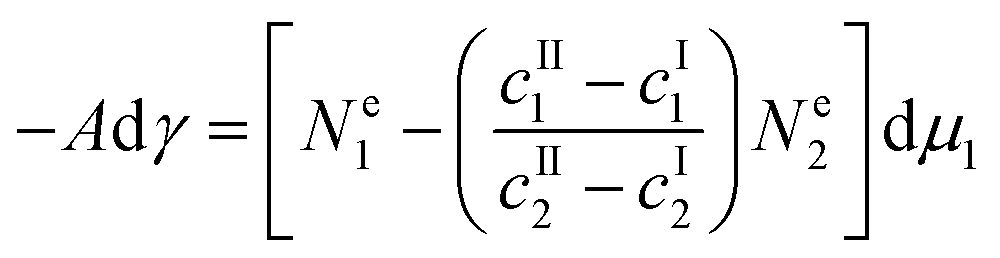
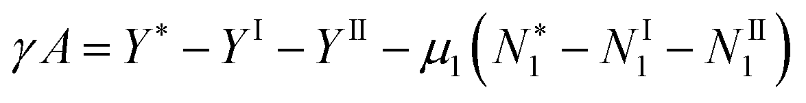
The first task before constructing a partially open ensemble is to specify the location of its boundary, the dividing surface. Following Gibbs, the boundary is positioned in such a way that the surface excess of the solvent becomes zero.10,46 This necessitates us to start from a set of Gibbs–Duhem equations for solvent and adsorbate by extending our previous paper.46 Let us consider the interface between the subsystems (phases) I and II, characterized by the surface area A and the surface tension γ. The entire system, denoted by *, is composed of I and II, as well as the interface between them, and the Gibbs–Duhem equation for the entire system is46| |  | (1) |
In addition to eqn (1), we need the Gibbs–Duhem equations for the phases I and II on their own, in the absence of the interface:46| | | NI1dμ1 + NI2dμ2 − VIdP + SIdT = 0 | (2) |
| | | NII1dμ1 + NII2dμ2 − VIIdP + SIIdT = 0 | (3) |
where V is volume, S is entropy, P is pressure, T is temperature, and μi and Ni are the chemical potential and number of the species i, respectively.
With this general setup, we can now consider any interface, such as gas–liquid, gas–solid, liquid–solid or liquid–liquid, so long as components in one of the phases can move around. Since the system's volume does not change due to the presence of the surface, we can use
to eliminate the d
P term from the combined
eqn (1)–(3), which yields
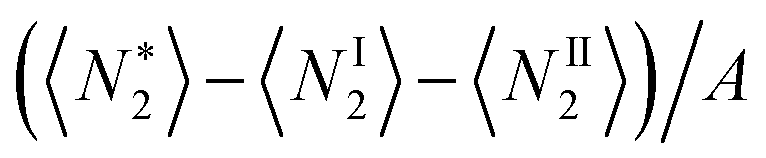
| | | −Adγ = Ne1dμ1 + Ne2dμ2 + (S* − SI − SII)dT | (5) |
where
Nei is the surface excess, defined as
| |  | (6) |
Using
eqn (2) and (3) in combination,
eqn (5) can be rewritten at constant temperature as
| |  | (7) |
where
cI1 and
cII1 are the concentrations of the species
i in phases I and II, respectively.
46
Now, we consider the spatial distribution of the solvent and adsorbate, whose surface excesses are related to the concentration profile  of species i along the surface normal by:23,24
| |  | (8) |
where
z is the coordinate along the normal, and
cαi is a weighted sum of the concentrations
cIi and
cIIi with arbitrary
α, defined as
| | | cαi = αcIi + (1 − α)cIIi | (9) |
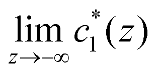
Eqn (8) defines the (experimentally determinable) Gibbs relative excess, which is indeed a convergent integral, whose value is independent of
α. However, due to the difference between

and

,

does not converge for any
α, because the integral kernel remains finite at least for one of the two (
z → ∞ or
z → −∞) sides. Hence, unlike solvation,
Ne1 and
Ne2 cannot be determined separately beyond their difference, but
eqn (8) is determinable.
10
2.2. Gibbs dividing surface and the equivalence of ensembles for the surface tension
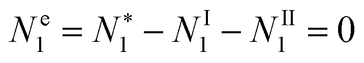
Positioning the Gibbs dividing surface appropriately can eliminate the solvent's surface excess (Ne1 = 0) so that we can focus exclusively on the distribution of adsorbates on the surface, as is well-known.10 Here, we implement this idea in an alternative manner, by introducing a set of partially-open ensembles satisfying Ne1 = 0.
As a preparation step, let us start from the grand canonical ensembles for the entire system and for the phases I and II, as
| | | Ω* = −PV* + γA ΩI = −PVI ΩII = −PVII | (10) |
Using
eqn (4), the volume conservation requirement, and the fact that
P is common to all three systems, we obtain
Based on the above preparatory discussion, now we introduce the thermodynamic function corresponding to the partially open ensemble,
Y, dependent on
N1,
μ2,
V, and
T,
via the Legendre transform:
where
τ refers to *, I, or II. Using
eqn (12) to convert the thermodynamic function from
Ωτ to
μ1Nτ1 and
Yτ yields
| |  | (13) |
Note that the same condition as required for the Gibbs dividing surface, namely a zero surface excess of the solvent

, is crucial to obtain the following relationship:
which may be considered to be the surface tension analogue of the equivalence of ensembles theorem for the chemical potential. The Gibbs dividing surface was implemented when
eqn (13) was transformed to
eqn (14). Using this procedure, the number of solvent molecules in the entire system

is determined uniquely from those in the subsystems
NI1 and
NII1. It should be noted that an intensive property of an interfacial system does not depend on the number of adsorbent (solvent) particles, and the Gibbs dividing surface is employed only for convenience. Still,
eqn (14) is useful for the subsequent developments. The formulae in Section 3 are expressed only in terms of the number of particles for the adsorbate species. This is because
eqn (14) does not involve terms with the chemical potential or particle number of the solvent.
Rewriting the Gibbs isotherm in terms of the set of partially-open ensembles will be helpful, because the Gibbs dividing surface has been incorporated automatically into the ensembles, thereby introducing the dividing surface without referring to concentration profile considerations, as will be discussed in Section 2.3. This was made possible by the Legendre transform, which makes the condition for the Gibbs dividing surface manifest in terms of thermodynamic functions, as seen in eqn (13). This takes advantage of the inter-dependence of μ1 and μ2viaeqn (2) and (3), which means that one out of two chemical potentials would suffice at constant temperature. This made it possible to choose the variables (N1, μ2, V, and T) instead of the conventional choice (μ1, μ2, V, and T). It is the choice of (N1, μ2, V, and T) or the partially-open ensemble that made the solvent surface excess  manifest in eqn (13).
Note that the arbitrary nature (i.e., Ne1 = 0) in the positioning of the dividing surface does not affect any of the subsequent theoretical development in the following, ensuring its applicability regardless of the nature of the interface.
2.3. Partially open ensembles for adsorption
Here, we introduce the partially open ensembles, and the corresponding partition functions, for the total system (τ = *), phase I (τ = I) and phase II (τ = II):| |  | (15) |
where λi is the fugacity of the species i,with  , where k is the Boltzmann constant, and the canonical partition functions are defined as
| |  | (17) |
where Λi is the thermal de Broglie wavelength, qi is the intramolecular partition function, and  and
and  denote collectively the coordinates of the species 1 and 2, respectively. When τ = *, Uτ should contain interactions coming from the atoms and molecules constituting the solid surface.
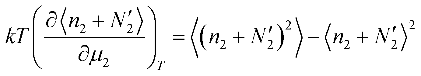
Now, we derive a relationship analogous to the Gibbs adsorption isotherm from this partially open ensemble. This is done by differentiating eqn (15) with respect to μ2, which is a natural variable, instead of μ1. The crucial step of this calculation is that by noting that Qτ(T,V,N1,N2) does not depend on μ2, we obtain
| |  | (18) |
Using
eqn (14) and (18), together with

, we obtain
| |  | (19) |
Thus, the adsorbate surface excess has been shown to come out naturally from the partially open ensembles. Such a re-derivation of the Gibbs adsorption isotherm is advantageous, because it does not have to consider the concentration profiles explicitly in order to introduce the dividing surface, meaning that it can be applied readily to rugged and porous surfaces.
3. The local subsystem approach to adsorption
Having generalized the concept of the dividing surface to incorporate rugged and porous surfaces in the previous section, now we are ready to clarify the localness of the adsorbate surface excess. To do so, we extend our recent statistical thermodynamic approach to solvation22,23,38 to the interface. Such a careful introduction of a local subsystem at the interface is beneficial in clarifying the behaviour of adsorbates, considering especially the much-discussed notion of interface “phases” or “complexion”.47–51 This generalization clarifies the requirements for the adsorbate surface excess to satisfy a condition analogous to thermodynamic stability. Most importantly, adsorbate fluctuation localized in the interfacial subsystem can be shown to be introduced through this section.
3.1. The “local” subsystem and the Gibbs isotherm
The partially open ensembles in Section 2 enabled us to focus exclusively on the adsorbate's surface excess, without the need to consider the solvent distribution explicitly to introduce the Gibbs dividing surface. However, the resultant expression (eqn (19)) is still inconvenient for application, and this can be appreciated from the following consideration:  does not depend on the system size as long as the systems are macroscopic, whereas
  , 〈NI2〉/A and 〈NII2〉/A all scale with the system size, which can be seen easily by extending the system thickness along the z axis.
Adopting a larger macroscopic set of systems simply means an expansion in volume of the bulk, in which adsorbate distribution is not affected by the surface. Indeed, surface phenomena are confined within a certain range of distance from the surface; focusing our attention exclusively within that range facilitates the analysis of an adsorption isotherm.
This motivated us to consider a set of subsystems that cover a relatively small range of z away from the dividing surface, where c2(z) deviates from cI2 on one side and from cII2 on the other side, as has been shown in a simplified manner in Fig. 1. More specifically, we need the three subsystems:
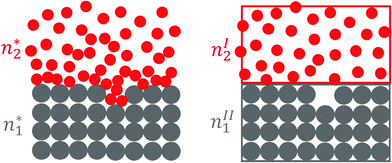 |
| | Fig. 1 A schematic illustration for the local subsystems in which the deviation of c2(z) from cI2 on one side and from cII2 on the other side is confined within the interfacial subsystem (left) with volume v*. Note that we have used the solid–liquid interface as an example here for simplicity, which means nI2 = 0 and nII2 = 0. The volume of the interface is v*, whereas those of the bulk subsystems are vI and vII, respectively. As shown in Sections 2 and 3, our theory is applicable to rugged or porous surfaces, even in the case when the surface melts. | |
(1) the “complete” local subsystem that contains a surface, whose volume is v*, and the numbers  and
and  ;
;
(2) the subsystem from phase I with vI, nI1 and nI2
(3) the subsystem from phase II with vII, nII1 and nII2
Here, we construct the subsystems from their macroscopic counterparts introduced in Section 2.3. Since the same procedure is applicable to all three subsystems, we present a general derivation without superscripts, which should be introduced when dealing with the subsystems *, I and II. Let us first note that there are  ways of choosing n2 molecules to be placed in the subsystem (with volume v) out of the N2 identical molecules in the system (with volume V). Therefore,
| |  | (20) |
where
| |  | (21) |
By introducing the number in the bulk phase defined by

,
eqn (20) and (21) can be rewritten, relative to the pure solvent partition function,
Γ(
T,
V,
N1,∞), as
| |  | (22) |
where
| |  | (23) |
Eqn (23) signifies the fugacity of inserting
n2 adsorbates within the local subsystem with a configuration
Xn2. Hence, the range of the integral in
eqn (22) is over the local subsystem. Consequently, we rewrite
eqn (22) and (23) as
| |  | (24) |
by introducing
| |  | (25) |
Then,
Rn is a physical quantity pertaining to the interface, since it involves the integration of fixed-configuration fugacity over the local subsystem.
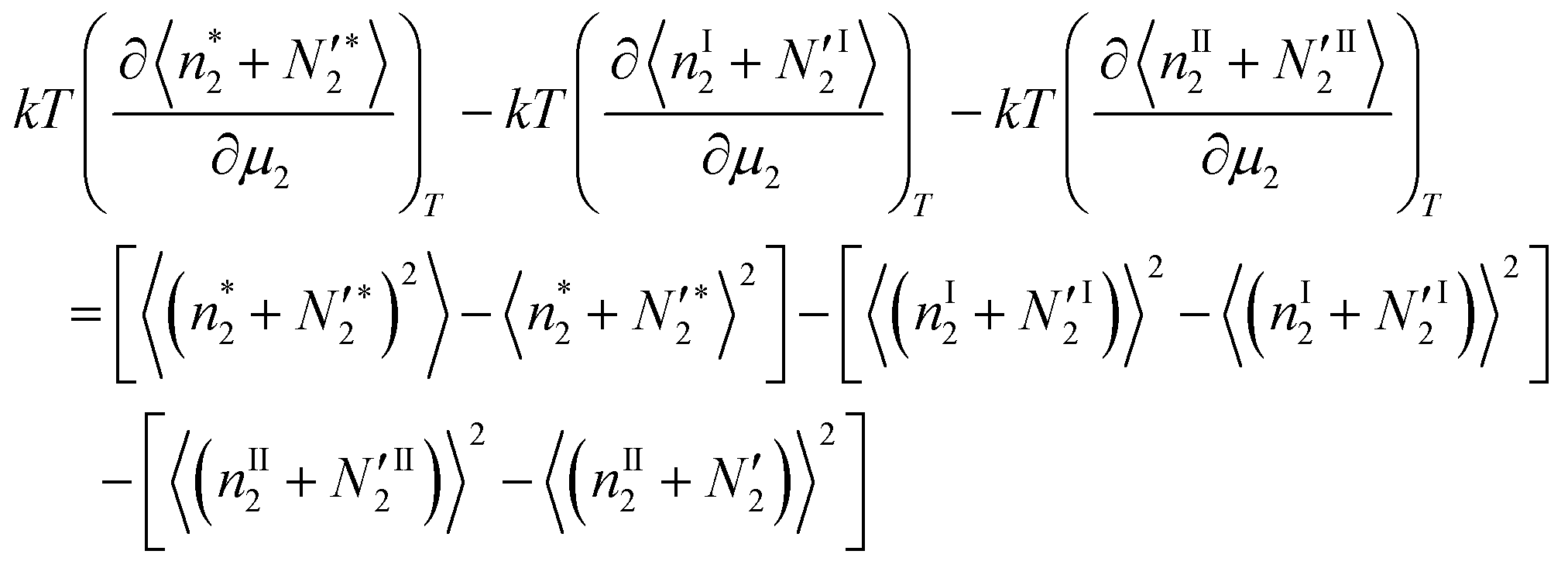
Let us first separate the local and bulk adsorbate numbers. To do so, eqn (18) can be rewritten, using the local–bulk division introduced by eqn (22) and (23), as
| |  | (26) |
By applying
eqn (26) for the three local subsystems whose volumes are chosen such that
v* =
vI +
vII, we obtain
| |  | (27) |
In the bulk phase, the distribution of adsorbate molecules is not affected by the presence of the surface. Hence, the bulk number conserves for our partially open systems
| |  | (28) |
Consequently, we obtain
| |  | (29) |
where
a2 is the activity of the adsorbate. Note that the right-hand side of
eqn (29) is independent of the choice of the interfacial region, in so far as the region is chosen such that the convergence of the density profile to the bulk values in phases I and II is assured within the volume
v* of the partially-open ensemble.
Thus, the Gibbs adsorption isotherm has been rewritten in terms of the number of adsorbate molecules in the local subsystems covering the correlation length of the surface.
3.2. Local fluctuation approach to adsorption
Adsorption isotherm models have been proposed with the aim of elucidating how the surface excess of an adsorbate depends on its activity. To address this question, we will demonstrate in Section 4 that the following derivative is useful.| |  | (30) |
which holds true for the *, I and II systems. The goal is to calculate the local number fluctuation. To do so, we calculate the μ2-derivative of  based on eqn (30). We start from
| |  | (31) |
The second term on the right-hand side of eqn (31) can be expressed as the difference of the bulk phase number fluctuations| |  | (32a) |
The left-hand side of eqn (31) can also be expressed as| |  | (32b) |
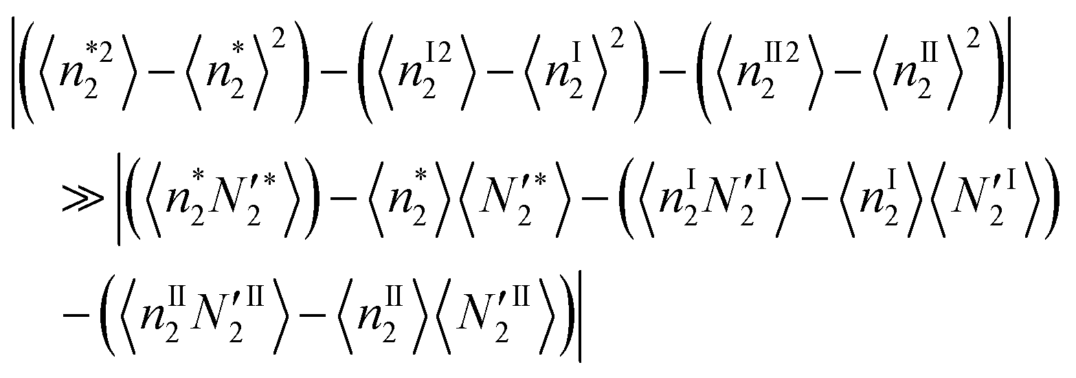
Using eqn (32a) and (32b), the bulk-phase contribution,  , can be shown to cancel out from both sides of eqn (31), which yields
| |  | (33a) |
Here, we postulate that the correlation between local and bulk phases is much smaller than the local fluctuation, namely| |  | (33b) |
meaning that the adsorbate–adsorbate interaction in the interfacial local system, which has been mediated by the presence of the interface, is much more significant than the change of adsorbate–bulk correlation brought about by the presence of an interface. Eqn (33b) is adopted only for the discussion at the end of Section 3.3; no other arguments are affected by eqn (33b). Using eqn (33b), the following formula can be derived for the ln![[thin space (1/6-em)]](https://www.rsc.org/images/entities/char_2009.gif) a2 dependence of the surface excess:
a2 dependence of the surface excess:| |  | (34) |
where a2 is the activity of the adsorbate. Note that the right-hand side of eqn (34) is independent of the choice of the volume of the partially open ensemble when the convergence of the density–density correlation to the bulk behavior is reached within that volume, in a similar manner with regard to eqn (29).
Thus, we have shown how the gradient of the adsorption isotherm can be linked to the local fluctuation.
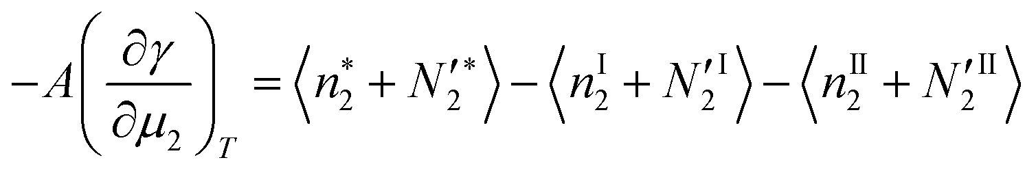
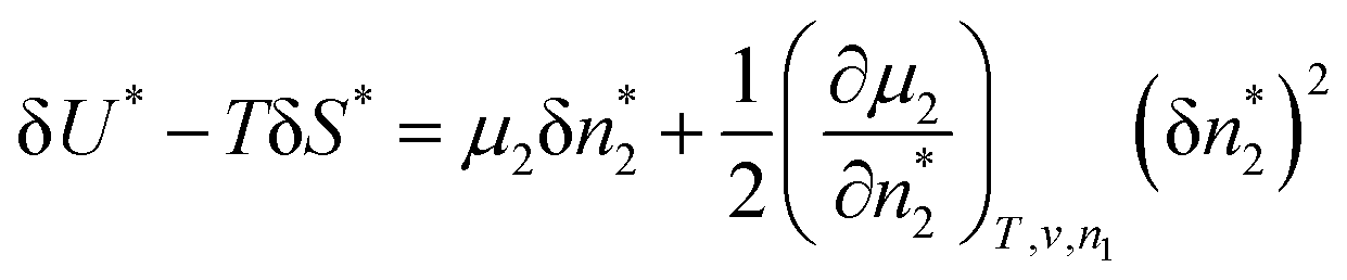
3.3. Thermodynamic stability condition for the local phase
Here, we establish the thermodynamic stability condition for adsorbates in the local subsystem. The local subsystem is much smaller than the entire system so a change of the subsystem's internal energy (δU*) does not affect the total energy of the entire system. Therefore,where δU′ is the change in the internal energy of the “surroundings”, namely, the entire system minus the local subsystem.52 Since both the volume of the local subsystem and the number of solvent molecules in the entire system are constant, δU′ can be expressed as| |  | (36) |
where δS′ and  are the increment of entropy and adsorbate number in the surroundings. Because of the conservation of this number,
  can be expressed in terms of the adsorbate number increment in the local subsystem,
  , as52
| |  | (37) |
To derive the thermodynamic stability condition, let the change be the deviation from equilibrium. Since the entropy of the local subsystem + the surroundings in equilibrium is at its maximum, a deviation from equilibrium results in an entropy decrease, such that
By combining
eqn (35)–(37),
eqn (38) can be rewritten as
52,53| |  | (39) |
By expanding the Helmholtz free energy,
| |  | (40) |
By combining
eqn (40) and (41), the equilibrium condition can be simplified as
| |  | (41) |
Since

is positive, we arrive at the following stability condition:
| |  | (42) |
where we have rewritten

as

in
eqn (42) based on the correspondence with statistical thermodynamics.
For eqn (42) to hold true, using
| |  | (43) |
it follows that
| |  | (44) |
is the stability condition for the adsorbates in the local subsystem. It goes without saying that
eqn (44) is a positive quantity, yet this fact needs to be emphasized in the context of the “interface phase” originally proposed by Gibbs.
54 For a surface excess (characterized by the excess number

) to be considered a phase, the excess number should behave just like a particle number in a given phase, such that
| |  | (45) |
By using
eqn (34),
eqn (45) is shown to be equivalent to
| |  | (46) |
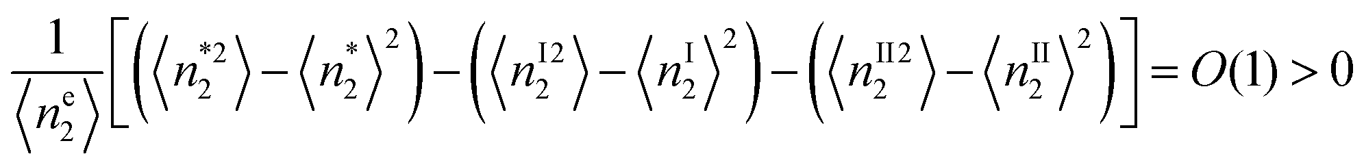
Eqn (46) means that the number fluctuation in the interfacial phase must be larger than those in the corresponding volumes in the bulk and surface interior phases. Eqn (46) is expressed only in terms of the quantities in the interfacial phase, which were derived based on eqn (33b) as an assumption of decoupling between the interface and bulk, which was needed to justify the view that a surface excess be treated as a phase. Eqn (34) and (46) do not affect the discussion in Sections 4 and 5.
Note that eqn (46) is not always satisfied, because eqn (45) applies only for adsorbates that accumulate increasingly as their chemical potential rises. However, if adsorbates are excluded from the interface, and increasingly so as their chemical potential rises, eqn (45) cannot be satisfied. Such a clarification is important, because whether an interface behaves like a phase has been carefully discussed in the literature.47–51 Our local subsystem approach to adsorption successfully sheds light on the range of applicability of this concept.
4. Determining adsorbate–adsorbate interaction from an isotherm
We have reformulated the Gibbs adsorption isotherm in terms of local interfacial subsystems. Because the dividing surface can be introduced without reference to a concentration profile, our approach is applicable for rugged and porous surfaces. These advantages enable us to generalize the two powerful approaches in solution chemistry, the Kirkwood–Buff19 and McMillan–Mayer35,55 theories, to interfacial local subsystems.
4.1. Adsorption of a single component onto a surface
Here, we consider simpler cases with abundant applications, namely the surface or interfacial adsorption of a single species, without consideration of the “solvent” species (i.e., species 1) described in Section 2. This can be achieved by equating species 1 as an adsorbent.
The advantage of our approach can be seen immediately when we consider a simple case of gas adsorption on the surface without penetration into the interior (we can consider a solid or liquid adsorbent – the general treatment of our partially open ensembles will turn out to be very useful here).
When the surface excess far exceeds that expected from its gas (“II”) phase density as well as from the lack of penetration into the interior (hence nI2 = 0), we can safely attribute the surface excess to the number of adsorbate itself, hence
| |  | (47) |
| |  | (48) |
Such a simplification cannot be achieved with ease when dealing directly with the macroscopic systems as in Section 2.
4.2. The generalized Kirkwood–Buff integral for adsorption
From now onwards, we shall only discuss gas adsorption on solid surfaces, and we omit the superscript * for simplicity. Here, we introduce a quantity analogous to the Kirkwood–Buff integral (KBI),22| |  | (49) |
and the excess number analogue of adsorbate around an adsorbate| |  | (50) |
in order to facilitate the analysis of vapour adsorption isotherms viaeqn (50). Using eqn (49) and (50), eqn (48) can be rewritten as| |  | (51) |
where a shorthand term,  , has been introduced.
Note that there is a difference between the common KBI defined in the solution phase and the KBI-analogue for adsorbates introduced here. First, the former is defined in the grand canonical ensemble whereas the latter is defined in the partially open ensemble. Second, even though N22 can be obtained exclusively from the observable quantity and does not depend on the dividing surface or v, the evaluation of G22 requires the adsorbate density c2 whose evaluation requires some information on surface thickness.
Nevertheless, the advantage of eqn (51) is in its facility of data analysis; c2G22 + 1 can be obtained directly from an adsorption isotherm as the gradient of a log–log plot (ln〈n2〉 plotted against lna2), yielding information regarding adsorbate–adsorbate interaction exclusively from experimentally-observable quantities. Such a directness and insight are in contrast with the conventional analysis of adsorption, which involves (a) a choice of isotherm and (b) data fitting.
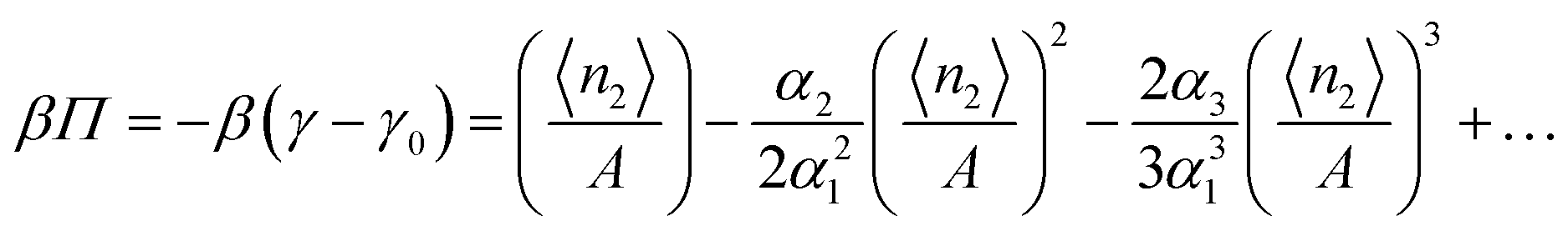
4.3. Virial expansion approach to the adsorption isotherm
Here, we show that an approach analogous to the McMillan–Mayer theory of solutions23,55,56 can be expanded to the interfacial local subsystem introduced in Section 3 and can be used to determine multiple-body interactions between adsorbates from the isotherm alone.
To achieve this aim, let us start from eqn (29). As mentioned above, the contributions from 〈nI2〉 and 〈nII2〉 are negligible for gas adsorption, so we can simplify it as
| |  | (52) |
By noting
a2 =
P2/
Po (
Po is the standard pressure),
eqn (52) can also be expressed in terms of the “spreading pressure”
Π,
57,58 as
| |  | (53) |
which inspires the construction of a theory analogous to the McMillan–Mayer theory. To do so, let us fit the adsorption isotherm with the following polynomial:
| |  | (54) |
Even though
eqn (54) is reminiscent of the three-parameter model for type II and III isotherms,
59 the theory presented here is a general one that is applicable to any isotherms (see below). Integrating
eqn (52) or (53), together with
eqn (54), yields
| |  | (55) |
Let us now express eqn (55) in terms of the adsorbate concentration. To do so, let us now invert eqn (54) as
| |  | (56) |
Substituting this back into
eqn (55) yields
| |  | (57) |
The analogy with the virial expansion shows that the second and third virial coefficients can be expressed as
| |  | (58) |
where
d is the thickness of the interfacial subsystem.
Thus, we have established how the virial coefficients defined in the interfacial local subsystem can be calculated from the adsorption isotherm. Unlike previous works,60–62 our theory is not specific to the geometry and dimensionality of the interface, and can therefore be applicable to rugged or porous surfaces.
4.4. Evaluating the critical adsorbate cluster size from an isotherm
A sharp increase of the adsorption isotherm is commonly referred to as the sign of a phase transition in the adsorbate phase.6,39 Here, we show that such an abrupt adsorption increase can be used to estimate the number of adsorbate molecules involved in the transition. Such a number will be referred to as the critical adsorbate cluster size.
To estimate the critical adsorbate cluster size, let us start from the stability condition, eqn (43), which states that  . Here, we consider the interfacial subsystem as composed of a set of independent, equivalent small systems; a small system should therefore contain a pore. We have recently established that the statistical thermodynamics of partially open ensembles can be applied to such a small system.13 It is easy for a small system to break the phase stability condition, which is possible merely when
| |  | (59) |
where
v is the volume of the small system. Using
eqn (50) and (51), the critical adsorbate excess number,
NC22, can be estimated from the gradient at the transition of the adsorption isotherm, as
| |  | (60) |
which is related to the critical aggregation size of the adsorbate, namely the number of adsorbates bound to an adsorbate molecule when the phase transition takes place (see Section 5.3).
5. Analysing adsorption isotherms
There has been a wide gap between general (statistical) thermodynamic theories of adsorption63,64 and fitting models for isotherms,65 both with a long history. By virtue of the local interfacial subsystem based on which the Kirkwood–Buff and McMillan–Mayer theories have been generalized, now we can embark on understanding what distinguishes different adsorption isotherm types.65 This will be achieved by quantifying adsorbate–adsorbate interactions in some of the most common adsorption models. Adsorbate–adsorbate interaction can be quantified equally in the absence of capillary condensation (Sections 5.1 and 5.2) and in its presence (Section 5.3).
Here, a clarification is in order: many simple isotherm models used for fitting, most notably the Langmuir and BET models, have been derived statistical thermodynamically.65 They are different from a general (statistical) thermodynamic approach,63,64 including our own here, in that they start from simple model assumptions, such as the number of adsorption sites and layers, as well as the binding constants thereunto.46,65 Our approach makes it possible to quantify adsorbate–adsorbate interactions across these models using the universal measures of the KBIs, excess numbers, and virial coefficients.
5.1. Determining the adsorbate–adsorbate Kirkwood–Buff integral from an isotherm
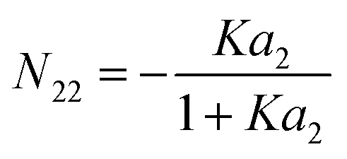
5.1.1. Langmuir isotherm (type I isotherm).
The Langmuir model65 is written in our notation as| |  | (61) |
which can be differentiated to yield| |  | (62) |
Using eqn (51) and (61), we obtain:| |  | (63) |
This can be simplified as| |  | (64) |
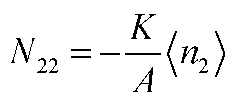
Note that N22 does not depend on A. The excess number at a2 = 0 is N22 = 0, showing that there is no correlation between water molecules, whereas at a2 → ∞, the excess number reduces to N22 = −1, reflecting the prohibition of site double occupancy. The excess number decreases linearly as the number of adsorbate molecules increases on the surface.| |  | (65) |
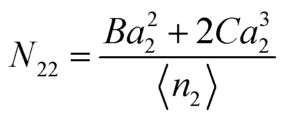
5.1.2. Polynomial isotherm (type II and III).
The following three-parameter model is used commonly to describe type II and III isotherms:65| | | 〈n2〉 = Aa2 + Ba22 + Ca32 | (66) |
At low a2, an isotherm with a concave curve is called type II whereas that with a convex curve is called type III.65 The difference between the two comes from the low a2 behaviour, through| | 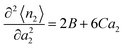 | (67) |
where concavity (type II) corresponds to B < 0 whereas convexity (type III) comes from B > 0. Using eqn (51), we obtain| |  | (68) |
Hence,| |  | (69) |
Eqn (69) shows that type II (B < 0) and type III (B > 0) exhibit an opposite behaviour in terms of adsorbate–adsorbate KBIs:
• Type II (concave) means N22 < 0: weaker interaction between the adsorbates;
• Type III (convex) means N22 > 0: stronger interaction between the adsorbates.
KBIs thus provide a clear picture of adsorbate–adsorbate interaction on the surface. The excess number is related to the total amount of adsorbate in the following manner:
| |  | (70) |
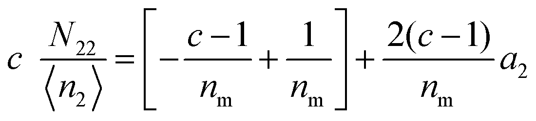
5.1.3. BET isotherm model.
The BET model65,66 is one of the most commonly used adsorption models, and it has the form:| |  | (71) |
where c is the BET parameter and nm is monolayer adsorption. This model can be conformed to eqn (51)via| |  | (72) |
Therefore, the adsorbate–adsorbate KBI,| |  | (73) |
diverges at  (since c is large, normally a negative number) and a2 = 1. Note that nm does not appear for adsorbate–adsorbate interaction. The relationship between N22 and n2 is:
| | 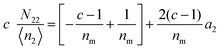 | (74) |
When c ≫ 1, eqn (73) becomes| |  | (75) |
which exhibits a large fluctuation at a2 → 1.
5.2. Virial expansion of adsorption isotherms
Fitting experimental data with common isotherm models (such as Langmuir or BET) can also be used to calculate the virial coefficients. To do so, the Maclaurin expansion of an isotherm is all that is required. For example, the Langmuir isotherm:| |  | (76) |
Using eqn (58), the virial coefficients are obtained as| |  | (77) |
B22 > 0 and B222 < 0 represent the unfavourable adsorbate–adsorbate interaction and favourable adsorbate–adsorbate–adsorbate interaction, respectively.
For the BET model, which can be used to fit type II and III isotherms,65 the virial coefficients can be calculated as well. This can be done by expanding the isotherm model as
| |  | (78) |
Using
eqn (58), the virial coefficients are obtained as
| |  | (79) |
The typical BET value would be in the order of 10
2, in which case
B22 > 0 and
B222 < 0, which again represent the unfavourable adsorbate–adsorbate interaction and favourable adsorbate–adsorbate–adsorbate interaction, respectively. The difference between Langmuir and BET is with regard to multiple-body interactions.
The approach based on the virial expansion, as presented above, provides an immediate insight into the difference in adsorbate–adsorbate interaction that gives rise to different types of adsorption. Types II and IV are concave downward whereas types III and V are concave upward. The concavity vs. convexity comes from the sign of α2 in the isotherm, see eqn (78), and considering that α1 > 0, we come to the following conclusion:
• Concave downward (types II and IV): α2 < 0, hence B22 > 0 and unfavourable adsorbate–adsorbate interaction;
• Concave upward (types III and V): α2 > 0, hence B22 < 0 and favourable adsorbate–adsorbate interaction.
Further classification of the different types of adsorption requires higher-order virial coefficients.
5.3. Estimating adsorbate aggregate size for capillary condensation
Types IV and V often exhibit hysteresis, as well as a steep change in the adsorption and desorption lines, which is considered to reflect capillary condensation.39 The type VI isotherm exhibits several step-like increases, attributed to a phase transition involving either adsorbates or adsorbents.39,67 Here, we show that the number of adsorbate molecules aggregated at the transition can be estimated viaeqn (60), using the adsorption isotherms of water on activated carbon fibres of different pore sizes.68
Adsorption isotherms of water vapour on hydrophobic activated carbon fibres have been measured by Nakamura et al.68 for the pore sizes of 1.1 nm, 1.0 nm and 0.6 nm, as shown in Fig. 2. The gradient calculated from a plot of lnn2 against lna2, as shown in Fig. 3, yields NC22 + 1. Here, we have chosen the region at which the gradient is the steepest for both adsorption and desorption lines. Using eqn (60) yields the excess number of water molecules around a water molecule, NC22, at the capillary condensation transition, as has been summarised in Table 1. The size of the aggregate, therefore, should be NC22 + 1, including the water molecule chosen for calculation of the excess number.
 |
| | Fig. 2 Adsorption (filled) and desorption (open) isotherms of water vapour on hydrophobic activated carbon fibres, measured by Nakamura et al.68 The pore sizes were 1.1 nm (black circles), 1.0 nm (red squares) and 0.6 nm (green diamonds). | |
 |
| | Fig. 3 Calculation of the excess number of water molecules around a water molecule, NC22, at the capillary condensation transition. For the identification of the isotherms, see Fig. 2. The steepest gradients (solid lines) were used as an input for eqn (60), which yields NC22. | |
Table 1 The size of water aggregate, NC22 + 1, obtained from the excess number of water molecules around a water molecule, NC22, at the capillary condensation transition. Calculated from experimental adsorption isotherms reported by Nakamura et al.68 (see Fig. 2). NC22 was calculated from the adsorption isotherm using eqn (60) (see Fig. 3)
| Pore size (nm) |
N
C22 + 1 (adsorption) |
N
C22 + 1 (desorption) |
| 1.1 |
8.41 |
10.4 |
| 1.0 |
5.61 |
9.75 |
| 0.6 |
2.46 |
2.46 |
The aggregate size, NC22 + 1, is calculated to be 2.46 for the activated carbon fibres with 0.6 nm pores. For reference, the maximum number of spheres that can be packed within a sphere, considering water as a sphere of 0.28 nm in diameter and simplifying a pore as a sphere, is about two or three (the size ratio is very close to the point of transition between the two values),69 consistent with the aggregate size calculated here. The pores with 1.0 and 1.1 nm widths, under the same simplification, can fit 22 and 30 spheres of the size of water, respectively.69 These numbers are much larger than the aggregate sizes obtained from the isotherm (Table 1). Besides the discrepancies arising from geometrical simplification and ignoring hydrogen bonds between water molecules, this result may suggest that capillary condensation can take place without completely filling the cavity.
Adsorption onto 0.6 nm pores does not exhibit any hysteresis.68 However, 1.0 and 1.1 nm pores both exhibit hysteresis. That the aggregation number for the desorption line is larger than the adsorption line shows that a stronger pre-formed water–water interaction must be broken at once for desorption, whereas the filling of the pore is more gradual with weaker water–water interaction.
We have thus demonstrated that adsorbate–adsorbate interaction can be quantified from the isotherm alone, regardless of hysteresis and the capillary condensation transition.
6. Complementing models and simulation via a rigorous and general theoretical approach
The present paper, being an extension to adsorption of our successful approach to solvation,10,12,13 is distinct in that certainty, credibility and clarity of interpretation are guaranteed by the rigorous nature of the theory. In this section, in view of the involved derivations presented above, it may be useful firstly to summarise the key theoretical steps and their respective foundations that directly underpin the application to adsorption isotherms. The key steps are:
(1) introducing the Gibbs adsorption isotherm without referring to adsorbate concentration profiles, facilitating its application to cases involving rugged surfaces, cavities or adsorbent melting;
(2) introduction of a local subsystem for adsorbates.
These achievements are based on the following foundations, respectively:
(1) the Gibbs–Duhem equations for the bulk and adsorbent phases, plus the Legendre transformation;
(2) that the effect of a surface on adsorbate arrangement is confined within a finite distance from the surface.
Unlike the empirical or model-based approaches, our theory is founded only on general principles.
The second aim of this section is to clarify how our approach, based on rigorous statistical thermodynamics, stands in relation to other approaches more commonly found in the literature. Applying statistical thermodynamics to adsorption is far from straightforward because of its complexity. The commonly adopted approaches, based on statistical thermodynamics, can be classified chiefly into the following two categories: development of adsorption isotherm models6,43,46,65,70,71 and computer simulation.72–75
Some of the adsorption isotherm models, the first category, range from the classical ones such as Langmuir and BET46,65 to more modern ones for porous surfaces,6,43,70,71 and are they developed with an aim to capture the essence of the surface structure, adsorption site distribution and adsorbate–surface and adsorbate–adsorbate interactions. The diversity in the adsorption models in the literature reflects the variety in surface structure and adsorbate interactions that must have been studied. Such an approach has a clear advantage when the experimental adsorption isotherm can be successfully reproduced by the model and when the model assumptions reflect the surface structure and the behaviour of the adsorbates. However, this approach runs into difficulty when multiple different models can fit an experimental isotherm,76–79 or when, despite successful fitting, the assumptions do not reflect the reality of the system.9 This is when the alternative approach of ours, based on the principles of statistical thermodynamics free of model assumptions, can be useful in its ability to quantify adsorbate–adsorbate interactions directly from the isotherm data alone. In addition, there are other types of adsorption isotherms that are empirical in origin, without a basis in model assumptions (such as the polynomial isotherm described in Section 5.2.2). In this case, our statistical thermodynamic approach is indispensable in attributing a physical meaning to each of the parameters (see 5.2.2).
The second category is computer simulation.72–75 Molecular dynamics and Monte Carlo simulations are fundamentally a numerical implementation of statistical thermodynamics, based on a set of model assumptions on the interactions that atoms and molecules, which comprise the adsorbates and surface, are engaged in. Its advantage is in its ability to capture the configurations of an adsorbate in relation to a surface and other adsorbates in atomic and molecular detail. However, how real the atomistic and molecular picture from simulation can be is dependent on the accuracy of the force field model used in simulation.80,81 In addition, it is not always straightforward to connect the microscopic configurations with the overall behaviour of the system.82–84 This is where our fluctuation theory can be useful: KBIs and virial coefficients provide a useful overall measure of interactions by which experimental isotherms and molecular configurations from simulation can be compared.
Thus, we have shown that our alternative approach based on the generality of fluctuation statistical thermodynamics is complementary to both the model-based and simulation approaches to adsorption.10–13,22–26 This approach, promulgated in this paper for surface adsorption, has a track record of success in the solvation of small molecules and macromolecules, where simple models have caused much confusion over how and why the addition of a cosolvent can influence solubility, conformation, aggregation and assembly.10–13,22–26 Its ability to quantify interactions between a specific pair of species solely from experimental data provided a clear guideline with which the accuracy and realism of a model can be judged.10–13,22–26
7. Conclusion
Based on the principles of statistical thermodynamics, we developed a rigorous theory of adsorption, which enables a model-free quantification of adsorbate–adsorbate interactions directly from an isotherm. This was achieved by extending the Kirkwood–Buff (KB) and McMillan–Mayer (MM) theories to an interfacial local subsystem. Using the interfacial extension of KB theory, adsorbate–adsorbate interaction can be determined straightaway from the log–log plot of an isotherm, in terms of the excess number of adsorbates around an adsorbate. The extension of MM theory yields multiple-body interactions between adsorbates in terms of the virial coefficients. Both the excess numbers and virial coefficients can be evaluated also from the fitting parameters for the well-known adsorption models, such as the Langmuir and BET models, clarifying what these models actually signify.
Quantifying the adsorbate aggregate size involved in capillary condensation and interfacial phase transition directly from an isotherm was made possible by an extension of the thermodynamic stability condition to the interfacial local subsystem. This novel approach was applied to a series of adsorption isotherms of water on activated carbons of varying pore sizes from the literature, demonstrating that the adsorbate aggregate size changes with the pore size.
Thus, interactions between adsorbates can be quantified from the isotherm alone in the presence and absence of condensation and phase transition. This has led to an origin of the different adsorption isotherm classifications by IUPAC via multiple-body interactions between adsorbates. Thus, our approach is able to fill a gap between adsorption models and statistical thermodynamics of adsorption.
These achievements come from the fact that our adsorption theory has no limitations in application, including the challenging cases such as rugged surfaces, cavities or crevices, and adsorbent melting into or evaporating from the solid phase. The theory is also applicable for solid and liquid surfaces alike and equally for vapour and liquid adsorbates. These advantages were afforded by the partially-open “local” interfacial subsystems,38 as a generalization of our recent work on the similarity and difference between solvation and adsorption.10,13,24,85 Thus, the fluctuation theory is versatile both in solvation and adsorption in quantifying interactions and clarifying how solvents and adsorbates work.
Conflicts of interest
There are no conflicts to declare.
Acknowledgements
We thank Katsumi Kaneko for kindly sending us the experimental data and Steven Abbott for a careful reading of the manuscript. S. S. thanks the Gen Foundation for supporting the early stage of this investigation and Steven Abbott TCNF Ltd for a travel fund. N. M. is grateful to the Grant-in-Aid for Scientific Research (No. JP19H04206) from the Japan Society for the Promotion of Science and the Elements Strategy Initiative for Catalysts and Batteries (No. JPMXP0112101003) and the Fugaku Supercomputing Project from the Ministry of Education, Culture, Sports, Science, and Technology.
References
- J. Israelachivili and H. Wennerstrom, Nature, 1986, 379, 219–225 CrossRef.
- A. Verdaguer, G. M. Sacha, H. Bluhm and M. Salmeron, Chem. Rev., 2006, 106, 1478–1510 CrossRef CAS.
- M. Tang, D. J. Cziczo and V. H. Grassian, Chem. Rev., 2016, 116, 4205–4259 CrossRef CAS.
- C. H. Giles, D. Smith and A. Huitson, J. Colloid Interface Sci., 1974, 47, 755–765 CrossRef CAS.
- D. D. Do and H. D. Do, Appl. Surf. Sci., 2002, 196, 13–29 CrossRef CAS.
- L. Liu, S. J. Tan, T. Horikawa, D. D. Do, D. Nicholson and J. Liu, Adv. Colloid Interface Sci., 2017, 250, 64–78 CrossRef CAS.
- S. H. Madani, P. Kwong, F. Rodríguez-Reinoso, M. J. Biggs and P. Pendleton, Microporous Mesoporous Mater., 2018, 264, 76–83 CrossRef CAS.
- S. H. Madani, M. J. Biggs, F. Rodríguez-Reinoso and P. Pendleton, Microporous Mesoporous Mater., 2019, 278, 232–240 CrossRef CAS.
- B. Lian, S. De Luca, Y. You, S. Alwarappan, M. Yoshimura, V. Sahajwalla, S. C. Smith, G. Leslie and R. K. Joshi, Chem. Sci., 2018, 9, 5106–5111 RSC.
- S. Shimizu and N. Matubayasi, J. Phys. Chem. B, 2014, 118, 3922–3930 CrossRef CAS.
- S. Shimizu and N. Matubayasi, J. Colloid Interface Sci., 2020, 575, 472–479 CrossRef CAS.
- S. Shimizu, Proc. Natl. Acad. Sci. U. S. A., 2004, 101, 1195–1199 CrossRef CAS.
- S. Shimizu and N. Matubayasi, Phys. A, 2021, 563, 125385 CrossRef CAS.
- S. N. Timasheff, Proc. Natl. Acad. Sci. U. S. A., 1998, 95, 7363–7367 CrossRef CAS.
- V. A. Parsegian, R. P. Rand and D. C. Rau, Proc. Natl. Acad. Sci. U. S. A., 2000, 97, 3987–3992 CrossRef CAS.
- S. N. Timasheff, Proc. Natl. Acad. Sci. U. S. A., 2002, 99, 9721–9726 CrossRef CAS.
- S. N. Timasheff, Biochemistry, 2002, 41, 13473–13482 CrossRef CAS.
- S. Shimizu and C. L. Boon, J. Chem. Phys., 2004, 121, 9147–9155 CrossRef CAS.
- J. G. Kirkwood and F. P. Buff, J. Chem. Phys., 1951, 19, 774–777 CrossRef CAS.
- D. G. Hall, Trans. Faraday Soc., 1971, 67, 2516–2524 RSC.
- A. Ben-Naim, J. Chem. Phys., 1977, 67, 4884–4890 CrossRef CAS.
- S. Shimizu and N. Matubayasi, J. Phys. Chem. B, 2014, 118, 10515–10524 CrossRef CAS.
- T. W. J. Nicol, N. Matubayasi and S. Shimizu, Phys. Chem. Chem. Phys., 2016, 18, 15205–15217 RSC.
- S. Shimizu and N. Matubayasi, Phys. Chem. Chem. Phys., 2017, 19, 23597–23605 RSC.
- S. Shimizu and N. Matubayasi, Phys. Chem. Chem. Phys., 2017, 19, 26734–26742 RSC.
- S. Shimizu and N. Matubayasi, Phys. Chem. Chem. Phys., 2018, 20, 13777–13784 RSC.
- S. K. Kim and B. K. Oh, Thin Solid Films, 1968, 2, 445–456 CrossRef CAS.
- B. K. Oh and S. K. Kim, J. Chem. Phys., 1974, 61, 1797–1807 CrossRef CAS.
- B. K. Oh and S. K. Kim, J. Chem. Phys., 1974, 61, 1808–1812 CrossRef CAS.
- B. K. Oh and S. K. Kim, J. Chem. Phys., 1977, 67, 3416–3426 CrossRef CAS.
- B. K. Oh and S. K. Kim, J. Chem. Phys., 1977, 67, 3427–3436 CrossRef CAS.
- Y. K. Tovbin, Russ. J. Phys. Chem. B, 2010, 4, 1033–1045 CrossRef.
- E. Tronel-peyroz, J. M. Douillard, R. Bennes and M. Privat, Langmuir, 1989, 5, 54–58 CrossRef CAS.
- W. H. Stockmayer, J. Chem. Phys., 1950, 18, 58–61 CrossRef CAS.
- T. L. Hill, J. Chem. Phys., 1957, 26, 955–965 CrossRef CAS.
- T. L. Hill, J. Chem. Phys., 1959, 30, 93–97 CrossRef CAS.
- T. L. Hill, J. Chem. Phys., 1961, 34, 1974–1982 CrossRef CAS.
- S. Shimizu and N. Matubayasi, Phys. Chem. Chem. Phys., 2016, 18, 25621–25628 RSC.
- T. Horikawa, D. D. Do and D. Nicholson, Adv. Colloid Interface Sci., 2011, 169, 40–58 CrossRef CAS.
- D. Nicholson, J. Chem. Soc., Faraday Trans., 1974, 1, 238–255 Search PubMed.
- J. C. Liu and P. A. Monson, Langmuir, 2005, 21, 10219–10225 CrossRef CAS.
- P. A. Monson, Microporous Mesoporous Mater., 2012, 160, 47–66 CrossRef CAS.
- S. W. Rutherford, Langmuir, 2006, 22, 702–708 CrossRef CAS.
- R. M. Barrer and A. B. Robins, Trans. Faraday Soc., 1951, 47, 773–787 RSC.
- W. F. Saam and M. W. Cole, Phys. Rev. B: Solid State, 1975, 11, 1086–1105 CrossRef CAS.
-
R. Defay and I. Prigogine, Surface tension and adsorption, Longmans, London, 1966 Search PubMed.
- S. J. Dillon, M. Tang, W. C. Carter and M. P. Harmer, Acta Mater., 2007, 55, 6208–6218 CrossRef CAS.
- M. Baram, D. Chatain and W. D. Kaplan, Science, 2011, 332, 206–209 CrossRef CAS.
- J. Luo, Curr. Opin. Solid State Mater. Sci., 2008, 12, 81–88 CrossRef CAS.
- W. D. Kaplan, D. Chatain, P. Wynblatt and W. C. Carter, J. Mater. Sci., 2013, 48, 5681–5717 CrossRef CAS.
- T. Frolov and Y. Mishin, J. Chem. Phys., 2015, 143, 044706 CrossRef CAS.
-
L. D. Landau and E. M. Lifshitz, Statistical Physics, Pergamon Press, London, 3rd edn, part I, 1986 Search PubMed.
-
I. Prigogine and R. Defay, Chemical Thermodynamics, Longmans, London, 1954 Search PubMed.
-
J. W. Gibbs, The collected works of J. W. Gibbs, Yale University Press, New Haven, CT, 1928 Search PubMed.
- W. G. McMillan and J. E. Mayer, J. Chem. Phys., 1945, 13, 276–305 CrossRef CAS.
-
T. L. Hill, Statistical Mechanics. Principles and Selected Applications, McGraw-Hill, New York, 1956 Search PubMed.
- A. L. Myers and J. M. Prausnitz, AIChE J., 1965, 11, 121–127 CrossRef CAS.
- H. H. Rowley and W. B. Innes, J. Phys. Chem., 1942, 46, 694–705 CrossRef CAS.
- M. Belhachemi and F. Addoun, Appl. Water Sci., 2011, 1, 111–117 CrossRef CAS.
- S. Ross and J. Olivier, J. Phys. Chem., 1961, 68, 608–615 CrossRef.
- W. Rudzinski and S. Sokolowski, Surf. Sci., 1977, 65, 593–606 CrossRef CAS.
- D. A. McQuarrie and J. S. Rowlinson, Mol. Phys., 1987, 60, 977–989 CrossRef CAS.
-
J. S. Rowlinson and B. Widom, Molecular Theory of Capillarity, Oxford University Press, Oxford, 1982 Search PubMed.
-
J. W. Cahn, The Selected Works of John W. Cahn, Wiley, New York, 2013 Search PubMed.
-
A. W. Adamson and A. P. Gast, Physical chemistry of surfaces, Wiley, 1997 Search PubMed.
- S. Brunauer, P. H. Emmett and E. Teller, J. Am. Chem. Soc., 1938, 60, 309–319 CrossRef CAS.
- K. Kaneko, J. Membr. Sci., 1994, 96, 59–89 CrossRef CAS.
- M. Nakamura, T. Ohba, P. Branton, H. Kanoh and K. Kaneko, Carbon, 2010, 48, 305–308 CrossRef CAS.
- T. Gensane, Les Cah. du LMPA J. Liouv., 2003, 188, 1 Search PubMed.
- S. Furmaniak, P. A. Gauden, A. P. Terzyk and G. Rychlicki, Adv. Colloid Interface Sci., 2008, 137, 82–143 CrossRef CAS.
- C. Buttersack, Phys. Chem. Chem. Phys., 2019, 21, 5614–5626 RSC.
- L. Sarkisov, A. Centineo and S. Brandani, Carbon, 2017, 118, 127–138 CrossRef CAS.
- C. L. McCallum, T. J. Bandosz, S. C. McGrother, E. A. Muller and K. E. Gubbins, Langmuir, 1999, 15, 533–544 CrossRef CAS.
- J. C. Liu and P. A. Monson, Ind. Eng. Chem. Res., 2006, 45, 5649–5656 CrossRef CAS.
- K. E. Brennan, J. K. Bandosz, T. J. Thomson and K. T. Gubbins, Colloids Surf., A, 2001, 187, 539–568 CrossRef.
-
A. Nilsson, L. G. M. Pettersson and J. K. Nørskov, Chemical Bonding at Surfaces and Interfaces, Elsevier, Amsterdam, 2008 Search PubMed.
-
F. V. Molina, Soil Colloids, CRC Press, Boca Raton, FL, 2016 Search PubMed.
- R. Kramer Campen, D. S. Zheng, H. F. Wang and E. Borguet, J. Phys. Chem. C, 2007, 111, 8805–8813 CrossRef.
- F. Brouers and F. Marquez-Montesino, Adsorpt. Sci. Technol., 2016, 34, 552–564 CrossRef CAS.
- C. Hölzl, P. Kibies, S. Imoto, R. Frach, S. Suladze, R. Winter, D. Marx, D. Horinek and S. M. Kast, J. Chem. Phys., 2016, 144, 144104 CrossRef.
- D. Horinek and R. R. Netz, J. Phys. Chem. A, 2011, 115, 6125–6136 CrossRef CAS.
- P. Krüger, S. K. Schnell, D. Bedeaux, S. Kjelstrup, T. J. H. Vlugt and J. M. Simon, J. Phys. Chem. Lett., 2013, 4, 235–238 CrossRef.
- R. Cortes-Huerto, K. Kremer and R. Potestio, J. Chem. Phys., 2016, 145, 141103 CrossRef CAS.
- D. M. Rogers, J. Chem. Phys., 2018, 148, 054102 CrossRef.
- S. Shimizu and N. Matubayasi, Biophys. Chem., 2017, 231, 111–115 CrossRef CAS.
|
| This journal is © the Owner Societies 2020 |
Click here to see how this site uses Cookies. View our privacy policy here. 
 Open Access Article
 This Open Access Article is licensed under a
  *a and
Nobuyuki
Matubayasi
*a and
Nobuyuki
Matubayasi


 of species i along the surface normal by:23,24
 and
and  ,
,  does not converge for any α, because the integral kernel remains finite at least for one of the two (z → ∞ or z → −∞) sides. Hence, unlike solvation, Ne1 and Ne2 cannot be determined separately beyond their difference, but eqn (8) is determinable.10
 , is crucial to obtain the following relationship:
 is determined uniquely from those in the subsystems NI1 and NII1. It should be noted that an intensive property of an interfacial system does not depend on the number of adsorbent (solvent) particles, and the Gibbs dividing surface is employed only for convenience. Still, eqn (14) is useful for the subsequent developments. The formulae in Section 3 are expressed only in terms of the number of particles for the adsorbate species. This is because eqn (14) does not involve terms with the chemical potential or particle number of the solvent.
 manifest in eqn (13).
 , where k is the Boltzmann constant, and the canonical partition functions are defined as
 and
and  denote collectively the coordinates of the species 1 and 2, respectively. When τ = *, Uτ should contain interactions coming from the atoms and molecules constituting the solid surface.

 , we obtain
 does not depend on the system size as long as the systems are macroscopic, whereas
  , 〈NI2〉/A and 〈NII2〉/A all scale with the system size, which can be seen easily by extending the system thickness along the z axis.

 and
and  ;
; ways of choosing n2 molecules to be placed in the subsystem (with volume v) out of the N2 identical molecules in the system (with volume V). Therefore,

 , eqn (20) and (21) can be rewritten, relative to the pure solvent partition function, Γ(T,V,N1,∞), as
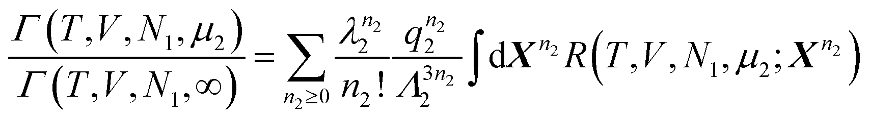


 based on eqn (30). We start from

 , can be shown to cancel out from both sides of eqn (31), which yields


 are the increment of entropy and adsorbate number in the surroundings. Because of the conservation of this number,
  can be expressed in terms of the adsorbate number increment in the local subsystem,
  , as52


 is positive, we arrive at the following stability condition:
 as
as  in eqn (42) based on the correspondence with statistical thermodynamics.


 ) to be considered a phase, the excess number should behave just like a particle number in a given phase, such that


 , has been introduced.


 . Here, we consider the interfacial subsystem as composed of a set of independent, equivalent small systems; a small system should therefore contain a pore. We have recently established that the statistical thermodynamics of partially open ensembles can be applied to such a small system.13 It is easy for a small system to break the phase stability condition, which is possible merely when


 (since c is large, normally a negative number) and a2 = 1. Note that nm does not appear for adsorbate–adsorbate interaction. The relationship between N22 and n2 is: