
 Open Access Article
 This Open Access Article is licensed under a
 Creative Commons Attribution 3.0 Unported Licence
The diffusion of doxorubicin drug molecules in silica nanoslits is non-Gaussian, intermittent and anticorrelated
Amanda
Díez Fernández
 a,
Patrick
Charchar
b,
Andrey G.
Cherstvy
c,
Ralf
Metzler
*c and
Michael W.
Finnis
*a
a,
Patrick
Charchar
b,
Andrey G.
Cherstvy
c,
Ralf
Metzler
*c and
Michael W.
Finnis
*a
aDepartment of Physics and Department of Materials, Imperial College London, London SW7 2AZ, UK. E-mail: m.finnis@imperial.ac.uk
bSchool of Engineering, RMIT University, Melbourne, Victoria 3001, Australia
cInstitute for Physics & Astronomy, University of Potsdam, 14476 Potsdam-Golm, Germany. E-mail: rmetzler@uni-potsdam.de
First published on 17th September 2020
Abstract
In this study we investigate, using all-atom molecular-dynamics computer simulations, the in-plane diffusion of a doxorubicin drug molecule in a thin film of water confined between two silica surfaces. We find that the molecule diffuses along the channel in the manner of a Gaussian diffusion process, but with parameters that vary according to its varying transversal position. Our analysis identifies that four Gaussians, each describing particle motion in a given transversal region, are needed to adequately describe the data. Each of these processes by itself evolves with time at a rate slower than that associated with classical Brownian motion due to a predominance of anticorrelated displacements. Long adsorption events lead to ageing, a property observed when the diffusion is intermittently hindered for periods of time with an average duration which is theoretically infinite. This study presents a simple system in which many interesting features of anomalous diffusion can be explored. It exposes the complexity of diffusion in nanoconfinement and highlights the need to develop new understanding.
1 Introduction
In recent years considerable progress has been made in discovering and characterising physical and biological systems that feature non-Brownian diffusion.1–9 Both single-molecule tracking experiments and computer simulations provide powerful means to study the diffusion dynamics in a variety of environments. In 2017, 3D single-molecule tracking experiments of large organic molecules diffusing on a functionalised silica surface clearly showed the presence of a hopping mechanism whereby the molecules undergo large displacements when momentarily detached and otherwise remain in states of low mobility.10 Previous 2D tracking experiments with smaller organic molecules indicated a similar behaviour.11 A recent study by Sarfati and Schwartz,12 which tracked rhodamine molecules in a thin film of water condensed on a silica substrate, is probably the most directly related to our present theoretical work. They observe anticorrelated diffusion near the surface and clearly identify non-Brownian, non-Gaussian motion. The molecule's dynamics was described by fractional Brownian motion (FBM), to account for the predominance of anticorrelated displacements, additionally interrupted by intermittent surface-adsorption events described by a continuous-time random walk (CTRW). In mathematical language, this corresponds to a subordination of the antipersistent motion to the adsorption times. Previous MD studies of diffusion of organic molecules in a solution confined between silica surfaces13,14 produced trajectories that were too short (<50 ns) to enable a detailed analysis within the framework of anomalous diffusion.Instead of a linear growth rate for the ensemble-averaged mean-squared displacement (EAMSD) of the particles, non-Brownian systems exhibit a nonlinear power-law scaling of the EAMSD, namely15–23
 | (1) |
In this work we study the diffusion of a doxorubicin molecule (DOX) in a nanofilm of water confined between two silica surfaces. DOX is considered one of the most effective anticancer drugs ever developed,27 being routinely used in treatment.28 However, its toxicity can lead to cardiac complications and failure,28 limiting the benefits of the therapy. One of the primary prevention strategies is to use liposomal DOX, whereby DOX is encapsulated within nanospheres.28 Commercialised in 1996, one such formulation was the first successful application of nanotechnology for drug delivery.27
Since mesoporous silica was first suggested as a suitable material to carry drug molecules in drug-delivery applications,29 a number of research groups have explored this option, as reviewed in ref. 30 and 31, partly because of the ease with which the silica surface can be functionalised and the porosity controlled. For example, the release rate of DOX from hollow mesoporous silica spheres can be manipulated by tuning the pore sizes, while a lower pH, such as that found in cancer cells, enhances the rate of release.32 Controlling the release rate is important in order to keep drug concentrations in the serum at an optimal level, thus improving the efficiency of the therapy by avoiding high- and low-concentration peaks.30 It is also important to achieve low release rates in the bloodstream and enhanced release at the target (exploiting, for example, the lower pH in cancer cells), in the absence of a more sophisticated design enabling other mechanisms to trigger release, such as, for example, that in ref. 33.
A central question in such applications is how efficiently DOX exits the silica carrier by diffusion. Though single-molecule tracking experiments of DOX diffusing inside mesoporous silica do exist,34 the data resolution is insufficient to provide a decisive insight regarding the underlying physical diffusion mechanism. Such information is important to understand better the effects of the molecular interactions and also to scale the observed dynamics to longer times and greater lengthscales. The motivation of our present work is therefore to better understand the diffusion of DOX in nanoconfinement in order to address this question. In our simulations, confinement is only between opposite planar surfaces, however this enables us to discover how nanoconfinement affects the diffusion process. The separation between the two surfaces was chosen to match the pore diameters of the nanoparticles reported in ref. 35, based on the synthesis method developed in ref. 36. The insights gained are interesting and unexpected: they could inform anomalous-diffuion studies of other systems as well as studies of DOX diffusing in cylindrical pores.
The paper is organised as follows. In Section 2 we present the details of the atomistic MD simulations. In Section 3 we present the main results and statistical data analysis. We consider the EAMSD and time-averaged MSD (TAMSD), the ageing properties of the underlying random walk, the distribution of particle displacements, the distribution of waiting times, and the position autocorrelation function. We also discuss possible mathematical and physical models of diffusion compatible with the data. In Section 4 we summarise our findings from the perspective of physical transport mechanisms and discuss some implications.
2 Details of computer simulations
Standard Gromacs 2018.2 was used to perform the MD simulations. The force field parameters describing the DOX molecule were defined using the Antechamber package37 and the general Amber force field (GAFF)38 for organic molecules. Discrete partial atomic charges were assigned using the constrained electrostatic potential energy methodology,39 consistent with the GAFF parameterisation strategy, and the quantum-mechanical electrostatic potential calculated with the Gaussian09 software.40 To achieve this, the structure of DOX was extracted from Protein Data Bank ID: 4DX7 (which is correctly protonated at physiological pH, see Fig. 1a) and the geometry optimised with the hybrid B3LYP functional and the 6-31G* basis set.41,42 Subsequently, the quantum-mechanical electrostatic potential of DOX was calculated using the Hartree–Fock formulation and the 6-31G* basis set, which is known to reproduce the relative free energies of solvation of organic molecules.43 Finally, a least squares procedure is used to fit a charge to each atomic centre in the molecule.39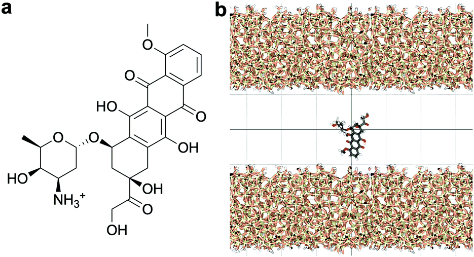 | ||
| Fig. 1 (a) Chemical representation of the doxorubicin (DOX) molecule. (b) Schematic of the silica-DOX system after equilibration. The background grid has a cell size of 1 nm. Water molecules and ions are not shown. | ||
To simulate the silica surface we used the INTERFACE force field,44,45 known to be suitable for simulations of biomolecules in solution in contact with, for instance, metals and ceramics. The force field is compatible with TIP3P46 and flexible SPC water models; the possibility to combine the silica surface with a flexible SPC water model is an advantage compared to the other commonly used silica force field for simulating organic molecules near silica,47 which is only compatible with TIP3P water.
One of these water models SPC/Fw48 yields the self-diffusion coefficient of water similar to that measured experimentally.48,49 The TIP3P water model, in contrast, predicts a diffusion coefficient more than twice the experimental value.48,50 This enhanced water diffusivity is also known to affect the mobility of organic molecules: for example, the diffusivity of glucose in TIP3P water confined in a silica channel was overestimated by 30%.13 Another study of protein diffusivity in TIP3P and SPC/Fw water models further demonstrated the advantage of SPC/Fw50 and the SPC/Fw model was also used recently to study the interactions of amino acids with a calcium–carbonate surface.51
The structure of the amorphous silica surface was taken from the Surface Model Database created by the developers of the INTERFACE force field.45 The surface has 4.7 silanol groups per nm2 of which 0.45 silanols per nm2 are unprotonated; instead, the charge is compensated by a sodium ion. This type of surface is found in most porous silica immersed in a slightly acidic solution (above pH 5).45 The silica slab in our simulations has periodic boundary conditions, and its parallel surfaces are separated by a slab of water in the {x,y}-plane, see Fig. 1b. The initial positions of the water molecules were as defined by the Gromacs program gmx_solvate. We performed fifty MD simulations, each 1 microsecond long, of a single DOX molecule in 1304 molecules of water. The periodically repeated simulation cell is orthorhombic, having dimensions of 4.04 × 4.17 × 4.59 nm. Since there is no clear boundary between the water and solid phase, see Fig. 2, we measure the average position of the centre of mass (COM) of the surface hydrogen atoms during the trajectory and take this value to define the interface (indicated by the dashed lines in Fig. 2). With this reference position, the silica surfaces confining the drug molecule are 2.45 nm apart, see Fig. 1 and 2.
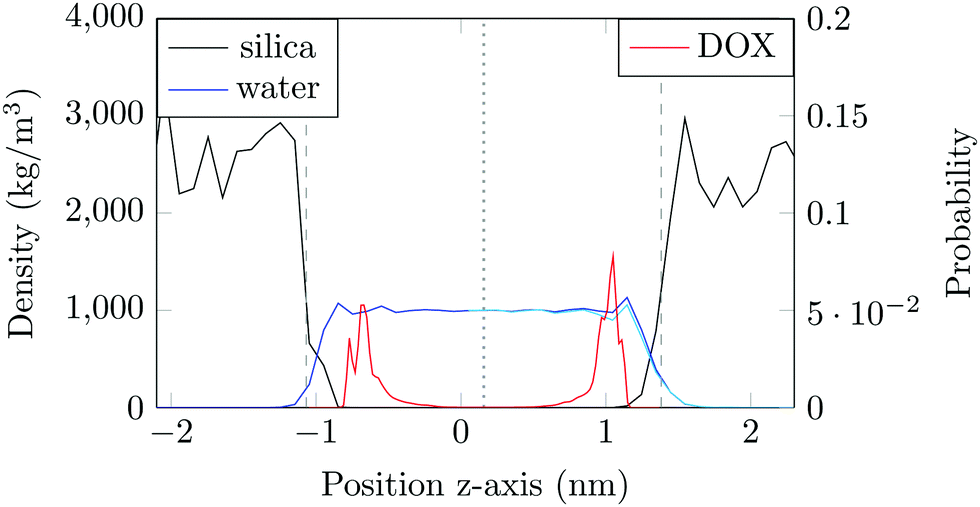 | ||
| Fig. 2 Water density (blue) and silica density (black) plotted across the channel (left axis). The water density when the DOX molecule is adsorbed to the right-hand surface is shown in light blue. The fraction of time the COM of the drug molecule occupies different heights, z, in the slit is shown in red (right axis). Average COMs of the surface hydrogen atoms are the dashed grey lines. The channel centre is the grey dotted line. | ||
The velocity Verlet scheme was used to integrate the equations of motion. The stretching of the covalent bonds involving hydrogen atoms in the system was constrained to be zero using the LINCS method.52 The correct treatment of this motion would require a quantum-mechanical treatment of the protons, while within the present classical treatment a fixed hydrogen–oxygen bond length provides a better representation than an oscillating bond.53 Without the need to resolve ultrafast oscillations, the time step of the simulation was set to 2 fs.
We first performed a short equilibration of the system using a Parinello–Rahman barostat in order to adjust the water density and remove a thin layer of vacuum introduced between the water and the silica. The next phase of equilibration was done separately for each simulation. Namely, the COM of the DOX molecule was tethered to the centre of the channel using a harmonic potential, in order to avoid surface adsorption before the start of the data collection. Velocities were randomly assigned to each atom of the system corresponding to a Maxwell distribution at 298 K. The temperature was controlled using a Nose–Hoover thermostat.54 After 5 ns of simulation time, the force restraining the COM was removed and the data recording started. This point marks the beginning of each simulated trajectory.
Velocity-scaling thermostats, such as the Nose–Hoover thermostat, are most suitable for approximating the real diffusive dynamics.55 However, when a rescaling thermostat is applied, the kinetic energy from the high-frequency modes is gradually transferred to low- or zero-frequency modes (such as the COM velocity). As a result, the system can “freeze” while it acquires a large translational velocity, a phenomenon called the flying ice cube effect.56 To avoid this, the COM velocities of the liquid, including DOX, Na+, Cl− and H2O species, and the atoms of the silica surface, were removed at every time step in the simulations. The fifty simulations were performed in single nodes of 32 CPUs, with a daily yield of 75 ns per trajectory.
3 Results
3.1 Surface adsorption leads to intermittent diffusion
The molecule was seen to intermittently adsorb to the surface and adopt a large number of configurations with respect to the surface, remaining in these positions of low mobility for long periods of time, often lasting hundreds of nanoseconds and in some cases for the entire one microsecond of simulation time. A sample trajectory is shown in Fig. 3. In Fig. 4 we depict four sample configurations in which the DOX molecule is close to the silica surfaces. In some cases the molecule's backbone is perpendicular to the surface (with some atoms locked in a pocket of the silica surface), see Fig. 4d, whereas in other situations it can be positioned flat with respect to the surface (Fig. 4a and b). When adsorbed the amplitude of the molecule's COM “oscillations” is often less than 1 Å along the {x,y}-plane, with sporadic larger oscillations, see inset in Fig. 5c, corresponding to the adsorbed molecule in Fig. 4a. The exact pattern of the oscillations depends on the adsorption configuration.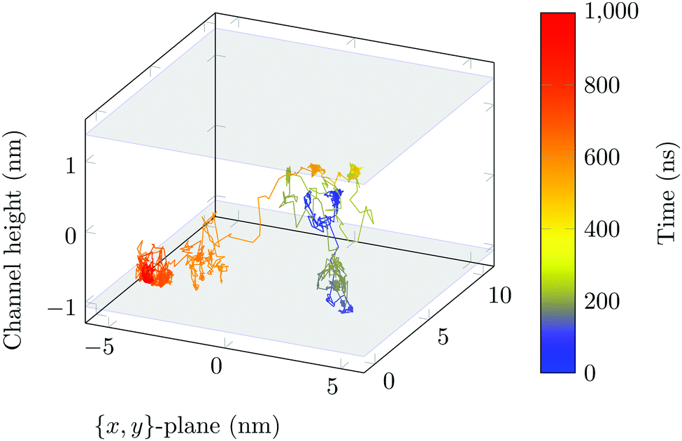 | ||
| Fig. 3 Sample 3D trajectory. Position of the COM of the DOX molecule is shown every 200 ps. The grey surface planes indicate the average position of the COM of the hydrogen surface atoms. The colour of the trajectory shows the time evolution (shown in ns). | ||
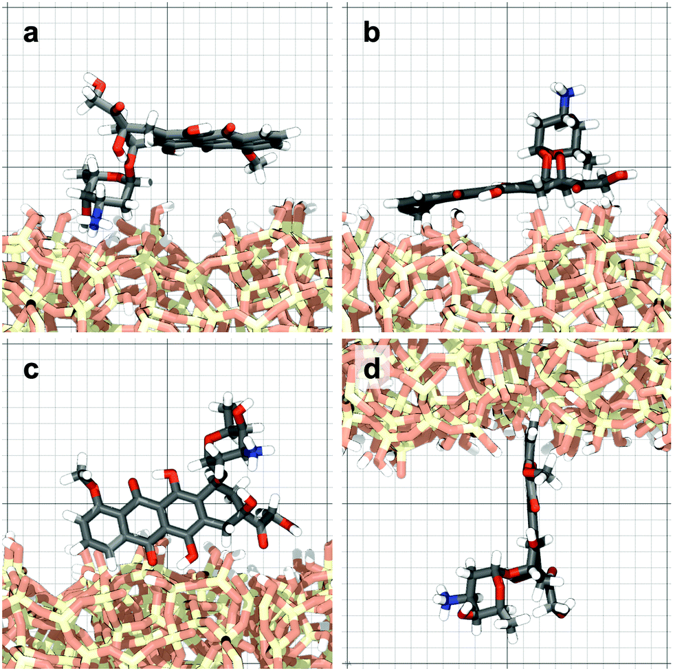 | ||
| Fig. 4 Four representative configurations of the drug molecule adsorbed on the silica surfaces. The background grid has a cell size of 1 nm. | ||
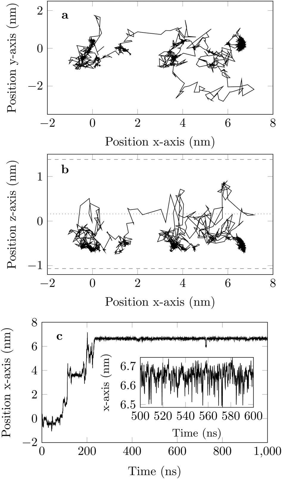 | ||
| Fig. 5 One trajectory of the DOX molecule projected in the (a) {x,y}-plane and (b) {x,z}-plane recorded for 1000 ns, with COM positions shown every 200 ps. The averaged COM position of the hydrogen-surface atoms is the pair of grey dashed lines. The channel centre is the dotted line. Panel (c) shows the time evolution of the position along the x-axis. | ||
Surface-detachment events are rare and often accompanied by quick lateral diffusion of the molecule in the channel, see Fig. 5 and 6. This two-state process with alternating periods of adsorbed motion and much less restricted bulk-like diffusion in the channel is physically similar to the picture of CTRWs:22,57 these feature distinct sojourn periods (here the bound states) and jump events. A similar phenomenon of intermittent, almost fully immobile states was observed, for instance, for the motion of Ka channels in the membranes of living human kidney cells.58–60
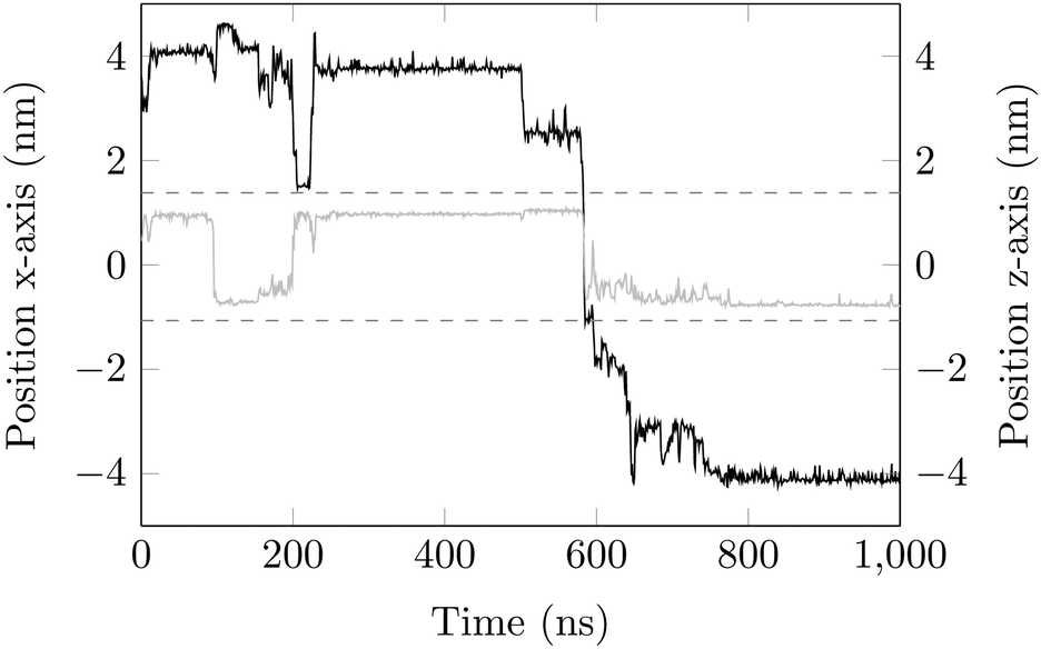 | ||
| Fig. 6 DOX displacement along the x-axis for one trajectory (black) and along the channel height (grey), with COM positions shown every ns. | ||
The density of water perpendicular to the channel axis varies non-monotonically as the silica surface is approached, first increasing slightly before decreasing steadily into the surface, which indicates a degree of water structuring typical for liquid–solid interfaces, see Fig. 2. When adsorbed, DOX displaces the water layer from the silica surface (notice the decrease in the water density in Fig. 2).
3.2 Mean-squared displacements show anomalous diffusion
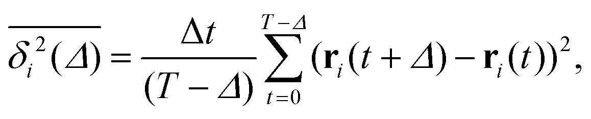
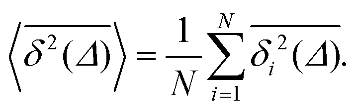
To quantify the above observations we plot the ensemble- and time-averaged MSD (EAMSD and TAMSD respectively) of DOX, see Fig. 7. The EAMSD is computed from | (2) |
 | (3) |
 | (4) |
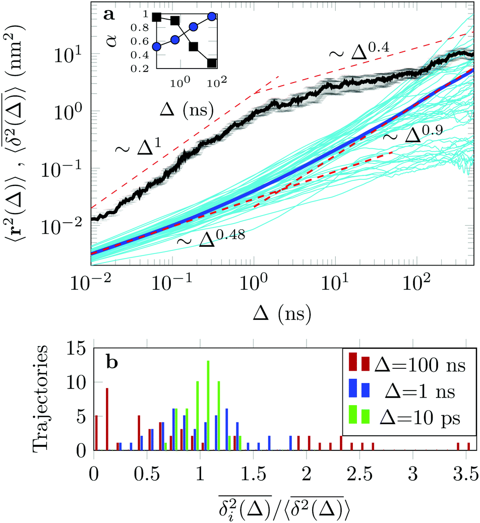 | ||
Fig. 7 (a) EAMSD (black), individual TAMSDs (light blue) and mean TAMSD (dark blue) of the drug molecule in the channel as a function of lag time. Asymptotes are indicated by the dashed lines. The error bars for the EAMSD curve are computed over 50 trajectories. The inset shows the variations of the time-local EAMSD and TAMSD scaling exponent, α (same colour coding). (b) Shows the amplitude-scatter distribution of individual TAMSDs  around their mean around their mean  . . | ||
The EAMSD starts linearly and after ≈1 ns turns into a subdiffusive behaviour with exponent α ≈ 0.4. In stark contrast, the mean TAMSD starts with exponent α ≈ 0.5 at short lag times and has an extended region of nearly normal diffusion at intermediate lag times, with α ≈ 0.9, see Fig. 7a. This disparity between EAMSD and TAMSD is often called weak ergodicity breaking22,61,62 and is not equivalent to non-ergodicty in the stronger mixing sense.63 Even a well defined process such as Brownian motion will display stochastic variations of the TAMSD from one trajectory to the next when measured over a finite time period.22,62 Similar fluctuations can also be seen in the single-trajectory power spectrum.64,65
For non-Brownian motion the distribution of such amplitude fluctuations are often characteristic to identify the specific underlying motion, e.g., to distinguish FBM from a CTRW process.22,66 The spread of the individual TAMSD is here quantified in Fig. 7b based on distributions of  . We observe that at very short lag times (Δ = 10 ps) the distribution is approximately bell-shaped but the maximum occurs just above the average. At lag time Δ = 1 ns the distribution has a clear dip in the probability at ξ = 1. At later lag times, at Δ = 100 ns, the difference between TAMSDs becomes more pronounced, with the emergence of traces with ξ > 3 and a large fraction of realisations with ξ close to zero. This broad distribution suggests subdiffusive CTRWs as a possible model for the observed diffusion. For subdiffusive CTRWs, however, theoretically the TAMSD should grow strictly linearly with lag time and the MSD should have a sublinear scaling with time,17–19,22 in contrast to our observations presented in Fig. 7. In fact the combination of CTRW with other processes, such as FBM and diffusion on a fractal, was observed in the single-particle tracking data from ref. 58 and 66.
Ageing is a another characteristic of subdiffusive CTRWs: the longer the time, T, allowed for the particle to move, the greater the probability it gets trapped for a long period of time (of the order of the recorded trajectory). In Fig. 5c, for example, the molecule displaces by more than 6 nm along the x-axis during the first 300 ns (intermittently undergoing short adsorption events) and then adsorbs in a very stable configuration (see Fig. 4a) for the remaining 700 ns. As these long periods of immobility are included in the sliding-window average, the TAMSD decreases.62 This is observed in Fig. 8a. A good fit by equation  , which describes the ageing behaviour of subdiffusive CTRWs,62 is achieved for α ≈ 0.66, see Fig. 8b. While only over a decade in time, the agreement with the scaling law ΔTα−1 is quite remarkable.
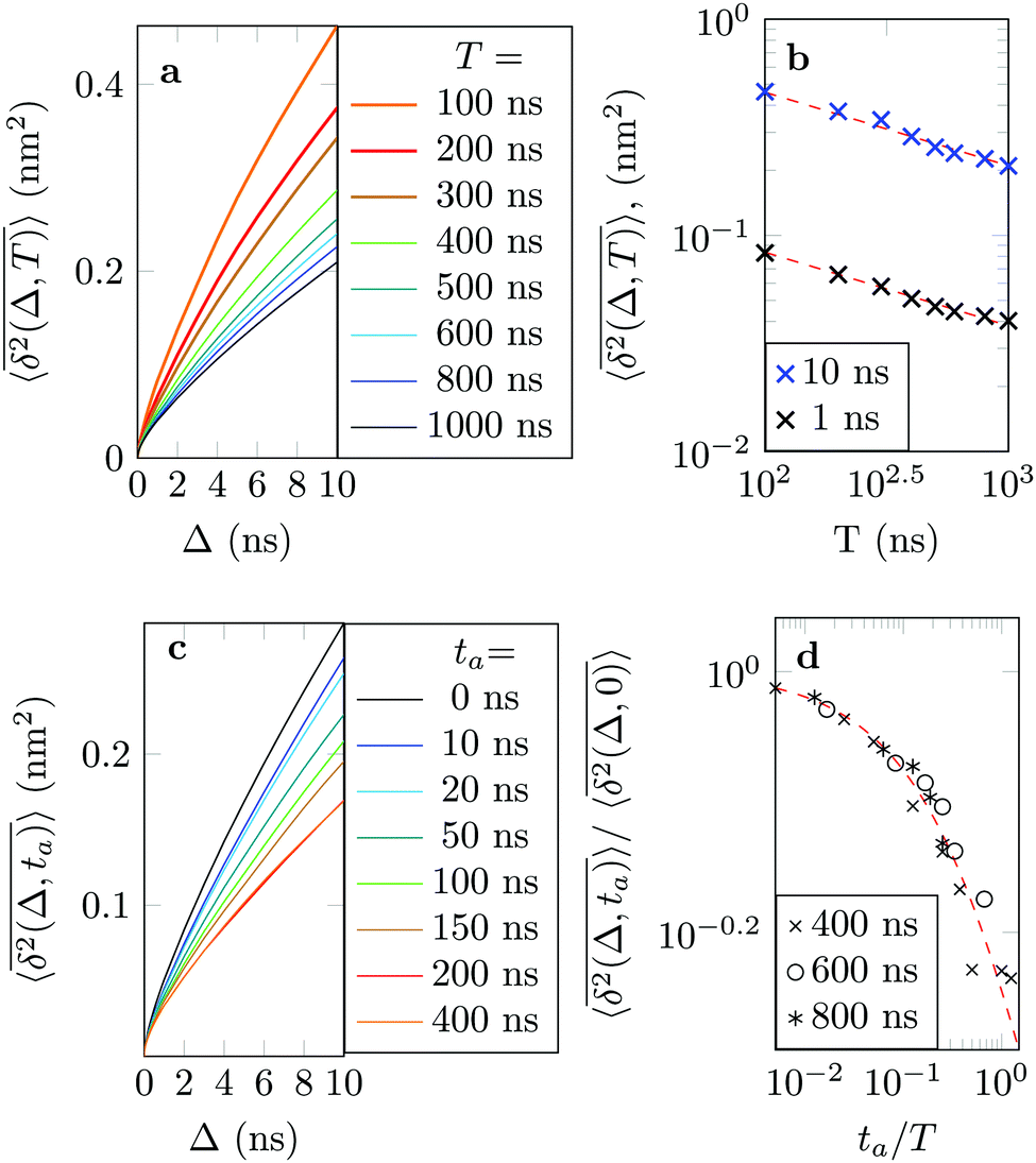 | ||
Fig. 8 (a) Mean TAMSD plotted for different trajectory lengths T. (b) Decrease in the mean TAMSD magnitude with increasing T, for Δ = 1 ns and Δ = 10 ns, the asymptotes,  , for α = 0.66 being shown as the dashed lines. (c) Mean TAMSD plotted for different ageing times ta, for trajectory segments of T = 400 ns. (d) Ratios of aged versus non-aged mean TAMSDs for different trajectory lengths T plotted versus the universal variable ta/T at Δ = 10 ns. The dashed asymptote is according to eqn (5) for the fit value α = 0.65. , for α = 0.66 being shown as the dashed lines. (c) Mean TAMSD plotted for different ageing times ta, for trajectory segments of T = 400 ns. (d) Ratios of aged versus non-aged mean TAMSDs for different trajectory lengths T plotted versus the universal variable ta/T at Δ = 10 ns. The dashed asymptote is according to eqn (5) for the fit value α = 0.65. | ||
Another manifestation of ageing is observed when an initial segment of the trajectory (termed the ageing time ta) is discarded and as a result the TAMSD decreases. In Fig. 8c, we take a segment of T = 400 ns and calculate the mean TAMSD when this segment starts at t = 0 (as in Fig. 8a) and at t = ta. As ta increases we observe a decrease in the mean TAMSD. The results after normalising the magnitude of the aged TAMSD to that of the non-aged for Δ = 10 ns and different values of T were plotted in Fig. 8d as a function of the universal rescaled variable ta/T and fitted to a well defined relation characteristic of subdiffusive CTRWs,67–69 with α = 0.65,
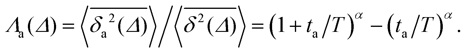 | (5) |
If we look at the percentage of time the molecule spends at different heights across the channel, Fig. 9, we see that during the first 100 ns the molecule is more likely (by an order of magnitude) to be in the central region of the channel compared to the last 100 ns of the trajectory. This is another illustration of the phenomenon discussed above: as the system evolves, the likelihood of finding the DOX molecule adsorbed in a very stable configuration increases.
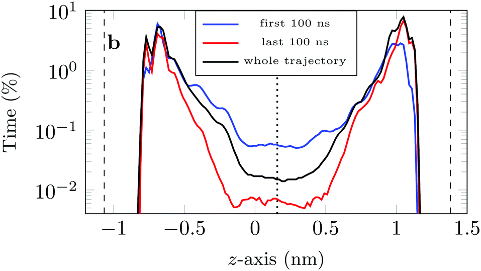 | ||
| Fig. 9 Percentage of time the COM of the drug molecule is found at a certain height in the channel, as calculated from all simulated trajectories for different intervals during the trajectory (the position was measured every picosecond and the positions grouped in 0.02 nm intervals). The dashed lines indicate the average position of the COM of the hydrogen surface atoms, whereas the dotted line indicates the centre of the channel. | ||
This is also clear from the sharp increase in the peak closest to the left surface and the overall increase in the probability of finding DOX close to the right surface.
3.3 Distribution of DOX displacements
The distribution of DOX displacements turns from an almost Gaussian shape at short times (1 ps) to a clearly non-Gaussian distribution at longer times in Fig. 10. A stretched Gaussian, which has been previously used to characterise non-Gaussian distributions of displacements70,71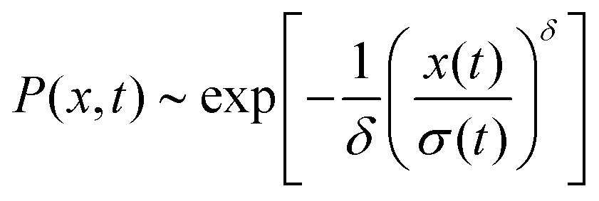 | (6) |
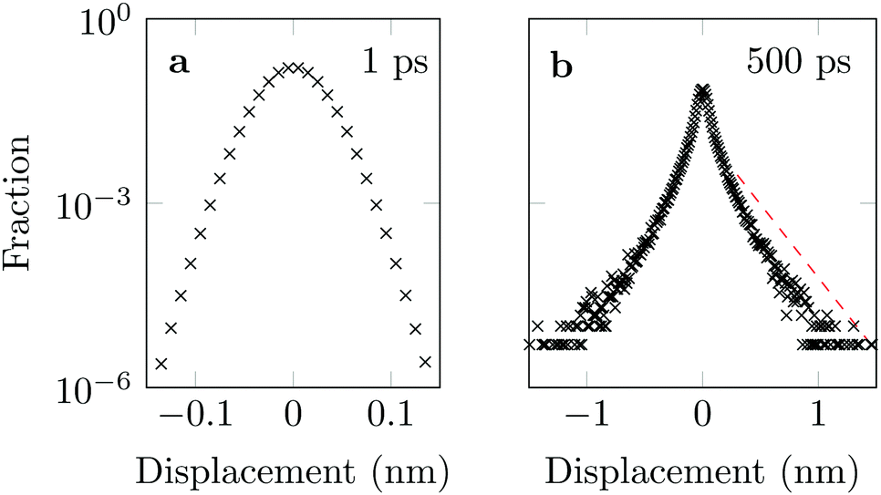 | ||
| Fig. 10 Characteristic displacements of the drug molecule after (a) 1 ps and (b) 500 ps. The dashed red line in (b) serves as reference indicating an exponential decay. | ||
As an alternative, we use the sum of four Gaussians with different amplitudes and widths. In order to obtain a fit independent of the bin width, the Gaussians were integrated over consecutive bin widths, producing discrete probability points, which were then fitted to the data. The probability of measuring a displacement of size, x, in the interval (a,b) is therefore given by
 | (7) |
The four Gaussian curves produce an excellent fit, as illustrated in Fig. 11. While the argument of Occam's razor would favour fewer adjustable parameters, the following discussion develops our reasoning to apply a description based on four Gaussians. Two Gaussian curves were insufficient to describe the tails of the distribution, three curves produced a good fit at short lag times but could not describe the tails correctly at larger times, while four produced an excellent fit for all computed distributions. Importantly, this choice yields a scaling of the standard deviation, encoded in this displacement distribution, consistent with the TAMSD growth, see Fig. 12a. Moreover, the fractional contribution of each Gaussian to the distribution remains approximately constant, see inset of Fig. 12a (compare ref. 3 and 6). Namely, the average weights of the fitted curves (in the order of increasing mobility) are ![[w with combining macron]](https://www.rsc.org/images/entities/i_char_0077_0304.gif) i = 44.8, 42.2, 11.8, and 1.2%. The narrowest Gaussian stops widening after ≈ 100 ps. The time evolution of the remaining three Gaussian curves could be fitted with the relation σi(t) ∼ tγi where γi ≈ 0.18, 0.32, and 0.43 respectively, see Fig. 12a. The spreading dynamics is therefore slower than Brownian motion (γ = 0.5) for all cases. The different spreading rates would explain the change in the distribution's shape observed in Fig. 10.
i = 44.8, 42.2, 11.8, and 1.2%. The narrowest Gaussian stops widening after ≈ 100 ps. The time evolution of the remaining three Gaussian curves could be fitted with the relation σi(t) ∼ tγi where γi ≈ 0.18, 0.32, and 0.43 respectively, see Fig. 12a. The spreading dynamics is therefore slower than Brownian motion (γ = 0.5) for all cases. The different spreading rates would explain the change in the distribution's shape observed in Fig. 10.
 | ||
| Fig. 11 Distribution of DOX displacements (crosses) with time lag 50 ps (a) and (b) and 200 ps (c) and (d), shown together with the fits by a combination of four Gaussian curves. Individual Gaussians are shown by the brown, red, yellow and green lines, while their sum is the solid blue curve. Displacements were measured separately along the x and y axis and their average evaluated afterwards. Dashed lines serve as reference indicating an exponential decay. | ||
 | ||
| Fig. 12 (a) Time evolution of the standard deviation for the data (crosses) and the four fitted Gaussian curves (coloured symbols). The dashed line shows the best fit to the data ∼t0.24. Best fits to the curves are 0.31t0.43, 0.3t0.32 and 0.3t0.18 for the green, yellow and red data points respectively. Inset: Shows the weights of each of the fitted Gaussian curves. The average values, i, for the green, yellow, red, and brown curves are: 1.2, 11.8, 42.2 and 44.8%, respectively and are indicated by the black lines. (b) Percentage of time the COM of the drug molecule is found at a certain height in the channel, as calculated from all simulated trajectories (the position was measured every picosecond and the position recorded in 0.02 nm intervals). The green, yellow, red, and brown areas occupy, respectively, ≈1.2, 12.9, 40.3, and 45.6% of the time. The dashed lines indicate the average position of the COM of the hydrogen surface atoms, whereas the dotted line indicates the centre of the channel. The colour coding is the same in both panels. | ||
From the macroscopic symmetry of the system, in the limit of infinitely long time and large simulation cell, the molecule would spend equal times in regions equally distant from the midplane of the channel, and we see in Fig. 12b that this symmetry of the distribution versus height in the channel is not exactly satisfied in the simulations. In Fig. 12b the channel is divided into four sections: a central region (green) and three regions (yellow, red and brown), each one closer to the surface than the previous one. The boundaries of these sections are chosen to match features in the distribution of time versus distance: for example, the regions closest to the surface end at the maxima of the distribution. This subdivision of the channel in four sections serves to illustrate our physical interpretation of the four fitted Gaussians by comparing their weights in the fit with the probability of finding the COM of the molecule at certain heights in the channel: 1 = 1.2% (DOX spends 1.2% of the time in green channel region), 2 = 12.9% (11.8% in the yellow region), 3 = 42.2% (40.3% in the red region) and 4 = 44.8% (45.6% in the brown region).
In the region highlighted in green, the molecule's COM is at least 7.8 Å from the surface; since DOX is ≈1.5 nm long, in this region the molecule is not in direct contact with the surface. The two Gaussians with the highest weights and slowest spreading dynamics correspond to the distribution peaks close to each surface.
Taken literally, this model would correspond to a division of the channel into layers 1, 2, 3 and 4, exhibiting four different mobilities of the diffusing molecule, between which the molecule hops at random intervals. Layer 1 would be a sub-channel centred on the mid-plane of the channel, where the mobility is highest, and layer 4 would be adjacent to the walls of the channel, where the mobility is most retarded by attachments. Layers 2 and 3 would fill the space between layers 1 and 4. Although there is no such clear discrete layering of the channel in our simulation, the physical picture we have is very similar if we interpret the four Gaussians to be a discrete representation of the continuously increasing mobility along the channel as a function of the distance of the molecule's COM from either surface.
3.4 Distribution of attachment times
A molecule is considered immobile if it stays for a given time τesc within a region of the {x,y}-plane with the escape radius resc. For these two parameters the values of τesc = 0.5, 1 ns and resc = 1, 2, 3, 5, and 10 Å were used in the analysis.We obtain long tails ∼τ−(1+γ) (leading to infinite theoretical sojourn times for γ < 1), see Fig. 13. Such scale-free distributions of immobilisation times are observed, e.g., in ref. 58 and 66. However the exponent γ is shown to decrease from ≈0.65 for resc = 3 Å to ≈0.1 for resc = 5 Å (both computed for τesc = 0.5 ns). Although functionally similar to the CTRW-process, the scaling exponent γ varies strongly, complicating a CTRW-based interpretation of this data, see below for more details.
 | ||
| Fig. 13 Normalised frequency of escape events from the circle of radius resc in the {x,y}-plane for resc = 3 Å (black, left axis) and resc = 5 Å (blue, right axis), with τesc = 0.5 ns for both panels. Both distributions are shown together in the inset (sharing the same y-axis). | ||
3.5 Displacement-autocorrelation function
A sensitive quantifier of the underlying diffusion process is the displacement autocorrelation function (ACF) of the drug molecules defined as | (8) |
In Fig. 14 we demonstrate that the displacement-autocorrelation function reveals antipersistent features, corresponding to the negative part of the correlation function. Physically this means that a displacement in one direction is likely followed by one in the opposite direction. This is consistent with the slower spreading dynamics of the Gaussian curves fitted to the displacement distributions when compared with Brownian motion. The data for ε = 10 ps is compared in Fig. 14 to a subdiffusive FBM process with a scaling exponent of α ≈ 0.47, producing a good fit. Note that a subdiffusive unconfined CTRW does not exhibit negative values in its displacement-autocorrelation function.17,22 The depth of the minimum decreases for larger ε values approaching a constant negative value asymptotically, see the inset of Fig. 14. In contrast, the FBM model predicts a minimum value independent of ε. Similar behaviour was recently reported for the diffusion of rhodamine molecules confined in a water layer between a silica surface and a vapour phase.12 The mininum value, in the FBM description, also approaches asymptotically a constant negative value, which is interpreted as an indication of true anticorrelation.12 Previously a dependence of the minimum value on ε had also been reported for the diffusion of nanoparticles in crowded dextran solutions, see ref. 72. Here, however, the minimum value approached zero asymptotically, which the authors attributed to a transient FBM process evolving towards Brownian motion.72,73
 | ||
| Fig. 14 Measured displacement-autocorrelation function (black crosses) compared with the theoretical FBM prediction for α = 0.47 and ε = 10 ps (red line). The inset shows the dependence of the measured displacement autocorrelation function on the binning size ε for values of ε of 1 ps (green), 10 ps (red), 100 ps (violet), 500 ps (blue) and 1000 ps (light blue). | ||
We measure the frequency with which n consecutive correlated displacements (or steps) of the drug molecule occur. For this calculation we consider the x and y directions separately. The results should be independent of the direction along which the steps were measured, so for optimal statistics an average was taken over both axes. The occurrence of each sequence of correlated steps is normalised by the number of times the steps change from being positively correlated to negatively correlated or vice versa. For example if we have the following six displacements: (+ + + − − −) we have two positively correlated steps (+ + +), followed by one negatively correlated step (+ −), followed by two positively correlated steps (− − −). The correlation therefore changed twice. In Fig. 15a we see that the decay in the correlation is independent of the time interval used to define the displacement, as is the case of the FBM model.
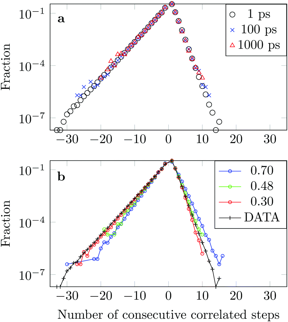 | ||
| Fig. 15 (a) Frequency of consecutive correlated displacements along simulated trajectories after intervals of 1 ps, 100 ps and 1000 ps. (b) Comparison with numerically simulated FBM trajectories with α = 0.30, α = 0.48 and α = 0.70. Positively correlated displacements are shown on the positive x-axis and negatively correlated displacements on the negative axis. | ||
The asymmetry of the curve, which exhibits a clear predominance of negatively correlated steps, highlights the already observed deviation from Brownian motion. The data coincides well with an FBM diffusion process with α = 0.30, see Fig. 15b, although there are some discrepancies at the tails. This could be due to the fact that we have a superposition of FBM processes or due to additional effects from the complex DOX-wall interactions.
4 Discussion
We studied in detail the motion of a single DOX molecule in a nanochannel with silica surfaces. Our simulations shed light on previously inaccessible time- and length-scales, providing new insight into diffusion in nanoconfinement.We observed that the DOX molecule adsorbs for prolonged periods on the silica surfaces and diffuses rapidly when detached. Once it adsorbs in a stable configuration it often remains in that position for the rest of the trajectory. This leads to so-called ageing, where on average the TAMSD is larger if measured at the beginning of the trajectory, (the molecule is less likely to have found a stable adsorption configuration), than when it is calculated from a segment later in the trajectory (when it is more likely to have adsorbed for a prolonged period of time). The motion of DOX, with its prolonged interruptions, therefore exhibits subdiffusive CTRW traits. The specific characteristics of the oscillatory motion induced by the presence of the surface could be causing the FBM-like character (with pronounced negative displacement correlations when adsorbed and almost vanishing correlations in the central region of the channel). The simulated data also exhibit properties that are not consistent with either of these two stochastic models. For example, while the overall shape of the autocorrelation function matches the FBM prediction, its minimum value depends on ε. A summary of the properties observed in our data compared to those of the FBM and CTRW models is shown in Table 1. Features of diffusion arising, as ours do, from different physical mechanisms within a system, have been observed previously.12,58,66,74
| Ergodicity | Ageing | Gaussianity | Min. ACF | |
|---|---|---|---|---|
| Data | No | Yes | No (4 Gaussians) | Negative value (ε dep.) |
| CTRW | No | Yes | No | Zero |
| FBM | Yes | No | Yes | Negative value (ε indep.) |
We fitted the diffusion of DOX by a time-independent superposition of four Gaussian processes, evolving at a rate slower than that associated with Brownian motion. The fit by four Gaussian curves is suggestive of the model discussed by Wang et al.,25 a particle intermittently undergoing different Gaussian processes leading to an overall non-Gaussian displacement distribution. In reality the molecule is moving through a continuum of Gaussian diffusion regimes parallel to the surfaces as it explores the width of the channel.
It has been demonstrated theoretically that ageing (specifically: a decrease in the TAMSD with increasing T as  ) can arise from the superposition of two Gaussian Brownian processes when a significant difference between the diffusion coefficients exists and the theoretical average time the diffusing object spends in the slow mode is infinite.75 Our system suggests a variation of this scenario, where we have a superposition of subdiffusive-FBM-like processes. At short lag times (in the order of several picoseconds), the difference in the displacements associated with these different processes is not pronounced, resulting in a FBM-like nonlinear TAMSD. As the lag times become longer the differences become larger and the α exponent approaches the CTRW value of 1.
In fact, the trajectories (see Fig. 6), might appear similar to those of the noisy CTRW,76 where the movements during periods of attachment are described by Ornstein-Uhlenbeck noise. In this system we might be observing a more complex motion due to the size of the molecule, with its 69 atoms sampling different parts of the channel simultaneously. Eliazar et al.,77 describe a scenario in which a superposition of Ornstein-Uhlenbeck processes can lead to FBM. A variation of this description could explain the origin of the observed FBM-type dynamics. Alternatively, as suggested in ref. 12, this FBM motion could be an indication that the water near the silica surface is viscoelastic.
Experimental studies measuring the percentage of DOX released from hollow mesoporous silica nanoparticles over a period of 30 hours showed that release was faster as the pore size was increased from 3.6 nm to 12.6 nm.32 As the pore diameter increases, the central region associated with fast diffusion increases leading to an overall increased diffusion rate. Furthermore, in a sufficiently large channel, Brownian motion would be recovered in the central region.
5 Outlook
In order to facilitate the design of new drug-carriers with optimal drug-release rates, it is useful to be able to extract the diffusion coefficient of DOX (or other drug molecules) through a variety of silica membranes (or other porous materials) either from single-molecule tracking experiments or computer simulations. The ultimate goal would be to produce mathematical expressions that predict the drug release rate at timescales that are relevant for medical applications and can be compared with experimental data.This study provides insight into the complexity of the diffusion process even in the simplest scenario, and shows that an analysis in which the diffusion coefficient is extracted simply from the classical Brownian motion equation, as in the single-molecule tracking experiments of DOX in silica nanopores,34 is not valid. Furthermore, this anomalous diffusion approach might prove advantageous compared to models that try to approach the problem by considering classical diffusion combined with an adsorption/desorption process (such as for example in ref. 78 and 79). Within the anomalous diffusion approach, all adsorption/desorption information is contained within the distribution of displacements and attachment times, the MSD and correlation analysis, thus avoiding the challenge of modelling the adsorption process explicitly.
We finally remark here that diffusion was modelled with a finite set of different Brownian motions with different diffusivities in the context of NMR signals,80 and an analogous model has recently been proposed for single-particle dynamics.81,82
Conflicts of interest
There are no conflicts to declare.Acknowledgements
A. D. F. and M. W. F. are grateful to Molly Stevens and Irene Yarovsky for helpful discussions. A. D. F. was supported through a studentship (Award reference: 1366033) in the Centre for Doctoral Training on Theory and Simulation of Materials at Imperial College London funded by the U.K. EPSRC. This work was carried out using the Imperial College Research Computing Service facilities, DOI: 10.14469/hpc/2232. R. M. acknowledges financial support by the Deutsche Forschungsgemeinschaft (DFG Grant ME 1535/7-1). R. M. also thanks the Foundation for Polish Science (Fundacja na rzecz Nauki Polskiej, FNP) for an Alexander von Humboldt Polish Honorary Research Scholarship.References
- M. J. Skaug and D. K. Schwartz, Ind. and Engin. Chem. Res., 2015, 54, 4414–4419 CrossRef CAS.
- D. Wang, R. Hu, M. J. Skaug and D. K. Schwartz, J. Phys. Chem. Lett., 2015, 6, 54–59 CrossRef CAS.
- C. E. Wagner, B. S. Turner, M. Rubinstein, G. H. McKinley and K. Ribbeck, Biomacromolecules, 2017, 18, 3654–3664 CrossRef CAS.
- T. J. Lampo, S. Stylianidou, M. P. Backlund, P. A. Wiggins and A. J. Spakowitz, Biophys. J., 2017, 112, 532–542 CrossRef CAS.
- S. Thapa, M. A. Lomholt, J. Krog, A. G. Cherstvy and R. Metzler, Phys. Chem. Chem. Phys., 2018, 20, 29018–29037 RSC.
- A. G. Cherstvy, S. Thapa, C. E. Wagner and R. Metzler, Soft Matter, 2019, 15, 2526–2551 RSC.
- S. Song, S. J. Park, M. Kim, J. S. Kim, B. J. Sung, S. Lee, J. H. Kim and J. Sung, Proc. Natl. Acad. Sci. U. S. A., 2019, 116, 12733–12742 CrossRef CAS.
- H. Yoshida, V. Kaiser, B. Rotenberg and L. Bocquet, Nat. Commun., 2018, 9, 1496 CrossRef.
- N. Bou-Rabee and M. C. Holmes-Cerfon, SIAM Rev., 2020, 62, 164–195 CrossRef.
- D. Wang, H. Wu and D. K. Schwartz, Phys. Rev. Lett., 2017, 119, 268001 CrossRef.
- M. J. Skaug, J. Mabry and D. K. Schwartz, Phys. Rev. Lett., 2013, 110, 256101 CrossRef.
- R. Sarfati and D. K. Schwartz, ACS Nano, 2020, 14, 3041–3047 CrossRef CAS.
- A. Ziemys, M. Ferrari and C. N. Cavasotto, J. Nanosci. Nanotechnol., 2009, 9, 6349–6359 CrossRef CAS.
- A. Ziemys, A. Grattoni, D. Fine, F. Hussain and M. Ferrari, J. Phys. Chem. B, 2010, 114, 11117–11126 CrossRef CAS.
- J.-P. Bouchaud and A. Georges, Phys. Rep., 1990, 195, 127–293 CrossRef.
- R. Metzler and J. Klafter, Phys. Rep., 2000, 339, 1–77 CrossRef CAS.
- S. Burov, J.-H. Jeon, R. Metzler and E. Barkai, Phys. Chem. Chem. Phys., 2011, 13, 1800–1812 RSC.
- E. Barkai, Y. Garini and R. Metzler, Phys. Today, 2012, 65, 29 CrossRef CAS.
- I. M. Sokolov, Soft Matter, 2012, 8, 9043–9052 RSC.
- M. J. Saxton, Biophys. J., 2012, 103, 2411–2422 CrossRef CAS.
- F. Höfling and T. Franosch, Rep. Prog. Phys., 2013, 76, 046602 CrossRef.
- R. Metzler, J.-H. Jeon, A. G. Cherstvy and E. Barkai, Phys. Chem. Chem. Phys., 2014, 16, 24128–24164 RSC.
- Y. Meroz and I. M. Sokolov, Phys. Rep., 2015, 573, 1–29 CrossRef.
- B. Wang, S. Anthony, S. Chul and S. Granick, Proc. Natl. Acad. Sci. U. S. A., 2009, 15160–15164 CrossRef CAS.
- B. Wang, J. Kuo, S. Bae Chul and S. Granick, Nat. Mater., 2012, 11, 481–485 CrossRef CAS.
- R. Metzler, Biophys. J., 2017, 112, 413–415 CrossRef CAS.
- Y. Barenholz, J. Controlled Release, 2012, 160, 117–134 CrossRef CAS.
- P. Vejpongsa and E. T. H. Yeh, J. Am. Coll. Cardiol., 2014, 64, 938–945 CrossRef CAS.
- M. Vallet-Regí, A. Rámila, R. P. Del Real and J. Pérez-Pariente, Chem. Mater., 2001, 13, 308–311 CrossRef.
- M. Vallet-Regí, M. Colilla, I. Izquierdo-Barba and M. Manzano, Molecules, 2018, 23, 47–66 CrossRef.
- N. Poonia, V. Lather and D. Pandita, Drug Discovery Today, 2018, 23, 315–332 CrossRef CAS.
- Y. Gao, Y. Chen, X. Ji, X. He, Q. Yin, Z. Zhang, J. Shi and Y. Li, ACS Nano, 2011, 5, 9788–9798 CrossRef CAS.
- J. Yang, D. Shen, L. Zhou, W. Li, X. Li, C. Yao, R. Wang, A. M. El-toni, F. Zhang and D. Zhao, Chem. Mater., 2013, 25, 3030–3037 CrossRef CAS.
- T. Lebold, C. Jung, J. Michaelis and C. Bräuchle, Nano Lett., 2009, 9, 2877–2883 CrossRef CAS.
- M. Hembury, C. Chiappini, S. Bertazzo, T. L. Kalber, G. L. Drisko, O. Ogunlade, S. Walker-Samuel, K. S. Krishna, C. Jumeaux, P. Beard, C. S. S. R. Kumar, A. E. Porter, M. F. Lythgoe, C. Boissière, C. Sanchez and M. M. Stevens, Proc. Natl. Acad. Sci. U. S. A., 2015, 112, 1959–1964 CrossRef CAS.
- H. Blas, M. Save, P. Pasetto, C. Boissière, C. Sanchez and B. Charleux, Langmuir, 2008, 24, 13132–13137 CrossRef CAS.
- J. Wang, W. Wang, P. A. Kollman and D. A. Case, J. Mol. Graphics Modell., 2006, 25, 247–260 CrossRef CAS.
- J. Wang, R. M. Wolf, J. W. Caldwell, P. A. Kollman and D. A. Case, J. Comput. Chem., 2004, 25, 1157–1174 CrossRef CAS.
- C. I. Bayly, P. Cieplak, W. D. Cornell and P. A. Kollman, J. Phys. Chem., 1993, 97, 10269–10280 CrossRef CAS.
- M. J. Frisch, G. W. Trucks, H. B. Schlegel, G. E. Scuseria, M. A. Robb, J. R. Cheeseman, G. Scalmani, V. Barone, G. A. Petersson, H. Nakatsuji, M. C. X. Li, A. Marenich, J. Bloino, B. G. Janesko, R. Gomperts, B. Mennucci, H. P. Hratchian, J. V. Ortiz, A. F. Izmaylov, J. L. Sonnenberg, D. Williams-Young, F. L. F. Ding, F. Egidi, J. Goings, B. Peng, A. PetroneT. Henderson, D. G. Ranasinghe, V. J. Gao, N. Rega, G. Zheng, W. Liang, M. Hada, M. Ehara, K. Toyota, R. Fukuda, J. Hasegawa, M. Ishida, T. Nakajima, Y. Honda, O. Kitao, H. Nakai, T. Vreven, K. Throssell, J. A. Montgomery, J. E. Peralta, F. Ogliaro, M. Bearpark, J. J. Heyd, E. Brothers, K. N. Kudin, V. N. Staroverov, T. Keith, R. Kobayashi, J. Normand, K. Raghavachari, A. Rendell, J. C. Burant, S. S. Iyengar, J. Tomasi, M. Cossi, J. M. Millam, M. Klene, C. Adamo, R. Cammi, J. W. Ochterski, R. L. Martin, K. Morokuma, O. Farkas, J. B. Foresman and D. J. Fox, Gaussian09 Revision C.01, 2010 Search PubMed.
- P. J. Stephens, F. J. Devlin, C. F. Chabalowski and M. J. Frisch, J. Phys. Chem., 1994, 98, 11623–11627 CrossRef CAS.
- A. D. Becke, J. Chem. Phys., 2014, 140, 18A301 CrossRef.
- L. F. Kuyper, R. N. Hunter and D. Ashton, J. Phys. Chem., 1991, 95, 6661–6666 CrossRef CAS.
- H. Heinz, T. Lin, R. K. Mishra and F. S. Emami, Langmuir, 2013, 29, 1754–1765 CrossRef CAS.
- F. S. Emami, V. Puddu, R. J. Berry, V. Varshney, S. V. Patwardhan, C. C. Perry and H. Heinz, Chem. Mater., 2014, 26, 2647–2658 CrossRef CAS.
- W. L. Jorgensen, J. Chandrasekhar, J. D. Madura, R. W. Impey and M. L. Klein, J. Chem. Phys., 1983, 79, 926–935 CrossRef CAS.
- E. R. Cruz-Chu, A. Aksimentiev and K. Schulten, J. Phys. Chem. B, 2006, 110, 21497–21508 CrossRef CAS.
- Y. Wu, H. L. Tepper, G. A. Voth and Y. Wu, J. Chem. Phys., 2006, 124, 024503 CrossRef.
- G. Raabe and R. J. Sadus, J. Chem. Phys., 2012, 137, 104512 CrossRef.
- K. Takemura and A. Kitao, J. Phys. Chem. B, 2007, 111, 11870–11872 CrossRef CAS.
- R. Innocenti Malini, A. R. Finney, S. A. Hall, C. L. Freeman and J. H. Harding, Cryst. Growth Des., 2017, 17, 5811–5822 CrossRef CAS.
- B. Hess, H. Bekker, J. C. H. Berendsen and G. E. M. J. Fraaije, J. Comput. Chem., 1997, 18, 1463–1472 CrossRef CAS.
- K. A. Feenstra, B. Hess and H. J. C. Berendsen, J. Comput. Chem., 1999, 20, 787–798 CrossRef.
- D. J. Evans and B. L. Holian, J. Chem. Phys., 1985, 83, 4069 CrossRef CAS.
- J. E. Basconi and M. R. Shirts, J. Chem. Theory Comput., 2013, 9, 2887–2899 CrossRef CAS.
- S. C. Harvey, R. K. Tan and T. E. Cheatham, J. Comput. Chem., 1998, 19, 726–740 CrossRef CAS.
- E. W. Montroll and G. H. Weiss, J. Math. Phys., 1965, 6, 167–181 CrossRef.
- A. V. Weigel, B. Simon, M. M. Tamkun and D. Krapf, Proc. Natl. Acad. Sci. U. S. A., 2011, 108, 6438–6443 CrossRef CAS.
- A. V. Weigel, M. M. Tamkun and D. Krapf, Proc. Natl. Acad. Sci. U. S. A., 2013, 110, E4591–E4600 CrossRef CAS.
- D. Krapf and R. Metzler, Phys. Today, 2019, 72, 48 CrossRef CAS.
- J.-P. Bouchaud, J. Phys. I, 1992, 2, 1705–1713 CrossRef.
- Y. He, S. Burov, R. Metzler and E. Barkai, Phys. Rev. Lett., 2008, 101, 058101 CrossRef CAS.
- J. L. Lebowitz and O. Penrose, Phys. Today, 1973, 26, 23–29 CrossRef.
- D. Krapf, E. Marinari, R. Metzler, G. Oshanin, X. Xu and A. Squarcini, New J. Phys., 2018, 20, 031001 CrossRef.
- D. Krapf, N. Lukat, E. Marinari, R. Metzler, G. Oshanin, C. Selhuber-Unkel, A. Squarcini, L. Stadler, M. Weiss and X. Xu, Phys. Rev. X, 2019, 9, 011019 CAS.
- S. M. A. Tabei, S. Burov, H. Y. Kim, A. Kuznetsov, T. Huynh and J. Jureller, Proc. Natl. Acad. Sci. U. S. A., 2013, 110, 4911–4916 CrossRef.
- J. H. P. Schulz, E. Barkai and R. Metzler, Phys. Rev. Lett., 2013, 110, 020602 CrossRef.
- J. H. P. Schulz, E. Barkai and R. Metzler, Phys. Rev. X, 2014, 4, 011028 Search PubMed.
- H. Krüsemann, R. Schwarzl and R. Metzler, Transp. Porous Media, 2016, 115, 327–344 CrossRef.
- A. G. Cherstvy, O. Nagel, C. Beta and R. Metzler, Phys. Chem. Chem. Phys., 2018, 20, 23034–23054 RSC.
- J.-H. Jeon, M. Javanainen, H. Martinez-Seara, R. Metzler and I. Vattulainen, Phys. Rev. X, 2016, 6, 021006 Search PubMed.
- M. Weiss, Phys. Rev. E: Stat., Nonlinear, Soft Matter Phys., 2013, 88, 010101 CrossRef.
- D. Molina-Garcia, T. Sandev, H. Safdari, G. Pagnini, A. Chechkin and R. Metzler, New J. Phys., 2018, 20, 103027 CrossRef.
- J.-H. Jeon, V. Tejedor, S. Burov, E. Barkai, C. Selhuber-Unkel, K. Berg-Sørensen, L. Oddershede and R. Metzler, Phys. Rev. Lett., 2011, 106, 048103 CrossRef.
- T. Miyaguchi, T. Akimoto and E. Yamamoto, Phys. Rev. E, 2016, 94, 012109 CrossRef.
- J.-H. Jeon, E. Barkai and R. Metzler, J. Chem. Phys., 2013, 139, 121916 CrossRef.
- I. Eliazar and J. Klafter, Phys. Rev. E: Stat., Nonlinear, Soft Matter Phys., 2009, 79, 021115 CrossRef.
- M. Kojic, M. Milosevic, N. Kojic, M. Ferrari and A. Ziemys, J. Serbian Soc. Comput. Mech., 2011, 5, 104–118 Search PubMed.
- A. Ziemys, M. Kojic, M. Milosevic, N. Kojic, F. Hussain, M. Ferrari and A. Grattoni, J. Comput. Phys., 2011, 230, 5722–5731 CrossRef CAS.
- J. Kärger, Adv. Colloid Interface Sci., 1985, 23, 129–148 CrossRef.
- A. Sabri, X. Xu, D. Krapf and M. Weiss, Phys. Rev. Lett., 2020, 125, 058101 CrossRef CAS.
- W. Wang, F. Seno, I. M. Sokolov, A. V. Chechkin and R. Metzler, New J. Phys., 2020, 22, 083041 CrossRef.
| This journal is © the Owner Societies 2020 |