
 Open Access Article
 This Open Access Article is licensed under a
 Creative Commons Attribution 3.0 Unported Licence
Quantum equilibration of the double-proton transfer in a model system porphine†
Guillermo
Albareda
 *ab,
Arnau
Riera
c,
Miguel
González
bd,
Josep Maria
Bofill
be,
Iberio de P. R.
Moreira
bd,
Rosendo
Valero
bd and
Ivano
Tavernelli
f
*ab,
Arnau
Riera
c,
Miguel
González
bd,
Josep Maria
Bofill
be,
Iberio de P. R.
Moreira
bd,
Rosendo
Valero
bd and
Ivano
Tavernelli
f
aMax Planck Institute for the Structure and Dynamics of Matter and Center for Free-Electron Laser Science, Luruper Chaussee 149, 22761 Hamburg, Germany. E-mail: guillermo.albareda@mpsd.mpg.de; guillealpi@gmail.com
bInstitute of Theoretical and Computational Chemistry, Universitat de Barcelona, Martí i Franquès 1, 08028 Barcelona, Spain
cICFO-Institut de Ciències Fotòniques, The Barcelona Institute of Science and Technology, Castelldefels (Barcelona), 08860, Spain
dDepartament de Ciència de Materials i Química Física, Universitat de Barcelona, Martí i Franquès 1, 08028 Barcelona, Spain
eDepartament de Química Inorgànica i Orgànica, Universitat de Barcelona, Martí i Franquès 1, 08028 Barcelona, Spain
fIBM Quantum, IBM Research – Zurich, 8803 Rüschlikon, Switzerland
First published on 14th September 2020
Abstract
There is a renewed interest in the derivation of statistical mechanics from the dynamics of closed quantum systems. A central part of this program is to understand how closed quantum systems, i.e., in the absence of a thermal bath, initialized far-from-equilibrium can share a dynamics that is typical to the relaxation towards thermal equilibrium. Equilibration dynamics has been traditionally studied with a focus on the so-called quenches of large-scale many-body systems. We consider here the equilibration of a two-dimensional molecular model system describing the double proton transfer reaction in porphine. Using numerical simulations, we show that equilibration indeed takes place very rapidly (∼200 fs) for initial states induced by pump–dump laser pulse control with energies well above the synchronous barrier. The resulting equilibration state is characterized by a strong delocalization of the probability density of the protons that can be explained, mechanistically, as the result of (i) an initial state consisting of a large superposition of vibrational states, and (ii) the presence of a very effective dephasing mechanism.
1 Introduction
There is currently a renewed interest in the derivation of statistical mechanics from the dynamics of a closed quantum system.1 In this approach, instead of assuming a priori that the system is in some mixed state, such as e.g. a micro-canonical ensemble, one describes it at all times using a pure state. One then seeks to show that, under reasonable conditions, the system behaves as if it was described by a statistical ensemble. In this way the use of statistical mechanics can be justified without introducing additional external degrees of freedom, such as e.g. thermal “baths”.A central part of this programme has been to understand the process of equilibration, i.e., how a constantly-evolving closed quantum system can share aspects typical to the relaxation towards a static equilibrium. The main insight relies on the fact2–4 that, if measurements are limited to small subsystems or restricted sets of observables, then “typical” pure states of large quantum systems are essentially indistinguishable from thermal states. It can then be shown5,6 that under very general conditions on the Hamiltonian and for nearly all initial states, the system will eventually equilibrate, in the sense that an (again, restricted) set of relevant physical quantities will remain most of the time very close to fixed, “equilibrium” values.
Quantum equilibration has been recently put within reach of experimental verification. Fueled by enormous improvements in experimental techniques it is now feasible to control quantum systems with many degrees of freedom. This is particularly true for the development of techniques to cool and trap ultracold atoms with optical lattices (giving raise to effective lattice systems)7–11 or suitable confinement potentials (that lead to effective low-dimensional continuous systems).12–15 Similarly, systems of trapped ions16,17 allow us to precisely study the physics of interacting systems in the laboratory.18–23 In such highly controlled settings, equilibration and thermalisation dynamics has been studied both experimentally24–28 and numerically, often with a focus on the so-called quenches, i.e. rapid changes of the Hamiltonian.29–37
While the most common notion of equilibration applies to thermodynamically large systems, we are here interested on the more general notion of equilibration on average1 (viz., a time-dependent property equilibrates on average if its value is for most times during the evolution close to some equilibrium value). This notion of equilibration applies also to small systems and we use it here to characterize the dynamics of an isolated molecular system. We consider a model system describing the double proton transfer reaction in the electronic ground state of porphine, a paradigmatic system in which the making and breaking of H-bonds occurs in an anharmonic Born–Oppenheimer potential-energy surface. Despite the approximations involved, the two dimensional analytical potential energy surface describing the coupled linear motions of the two protons serves well for the proof of principle discussed here. As it will be shown, for initial states with energies above the synchronous double-proton transfer energy barrier involving a large coherent sum of vibrational states, the isomerization dynamics can reach a long-lived quasi-stationary regime with associated physical quantities, such as the mean position or momentum, that remain close to fixed, “equilibrium”, values.
2 Definitions
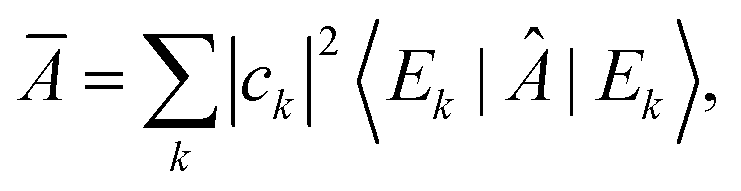
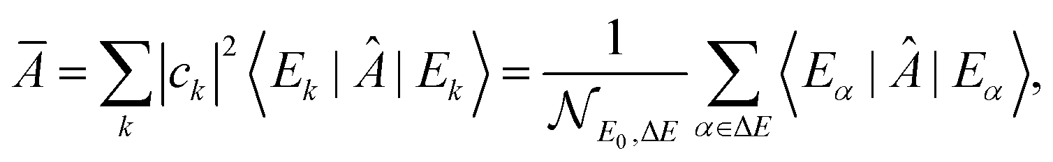
Equilibration is achieved when a measurable quantity, after having been initialised at a non-equilibrium value, evolves towards some value and then stays close to it for an extended amount of time. More precisely, given some observable A and a system of finite but arbitrarily large size, if its expectation value 〈Â(t)〉 equilibrates, then it must do so around the infinite time average,1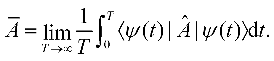 | (1) |
This notion of equilibration is compatible with the recurrent and time reversal invariant nature of unitary quantum dynamics in finite dimensional systems. To see that, let us assume a closed system whose state is described by a vector in a Hilbert space of dimension dT and whose Hamiltonian has a spectral representation 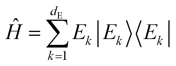 , where Ek are its energies and |Ek〉 are eigenstates of Ĥ.‡ Choosing units such that ħ = 1, the state at time t is then given by
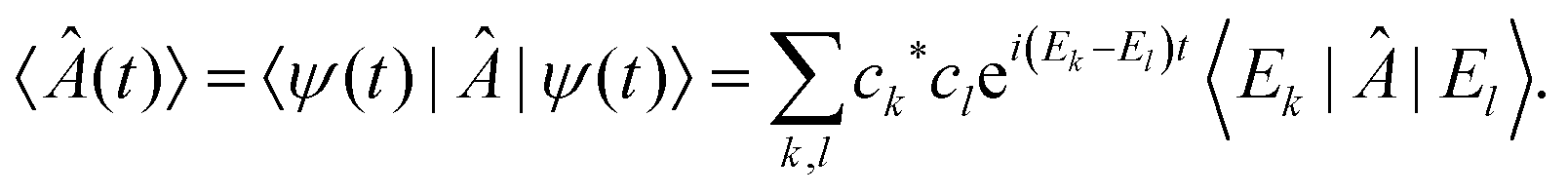
 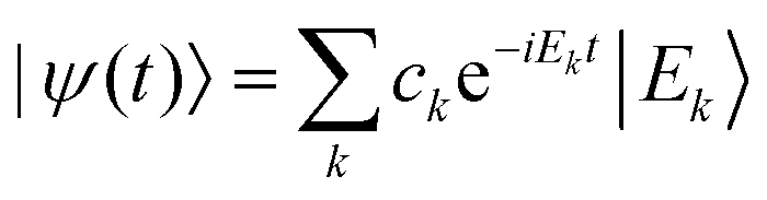 with ck ≡ 〈Ek|ψ(0)〉, and the expectation value of  can be written as:
 | (2) |
 | (3) |
 . Therefore, if the system relaxes at all, it must be to the following density matrix:
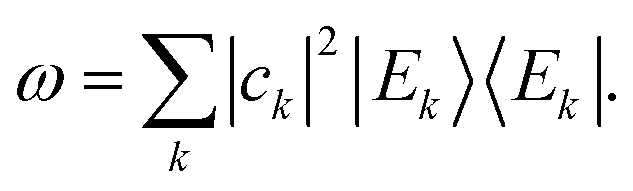 | (4) |
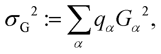
Sufficient conditions for equilibration in the sense defined above can be then defined in terms of the so-called effective dimension. Roughly speaking, the effective dimension is a measure of the number of significantly occupied energy eigenstates, and is defined as:
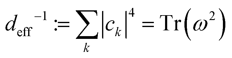 | (5) |
Provided that a given observable equilibrates, it was recently shown40 that the equilibration time can be related with a dephasing time τd as:
| Teq ∼ τd = π/σG. | (6) |
 | (7) |
![[capital G, script]](https://www.rsc.org/images/entities/char_e112.gif) = {(i,j):i, j ∈ {1,…dE}, i ≠ j}, and
= {(i,j):i, j ∈ {1,…dE}, i ≠ j}, and 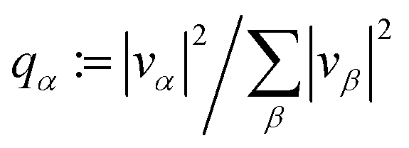 with vα = cj*Ajici/σA, and Aij := 〈Ei|A|Ej〉 are the matrix elements of A in the energy eigenbasis. The denominator σA = amax − amin is the range of possible outcomes, being amax(min) the largest (smallest) occupied eigenvalue of Â.
3 Porphine model
The above introduced concepts are now used to characterize the non-integrable model Porphine designed by Smedarchina et al.41 to describe the switch from synchronous (or concerted) to sequential (or stepwise) double-proton transfer.42,43 This model accounts for the motions of two protons (labeled 1 and 2) along coordinates R1 and R2, respectively, from the domains of the reactant (R) to the product (P) (see Fig. 1). The PES model is41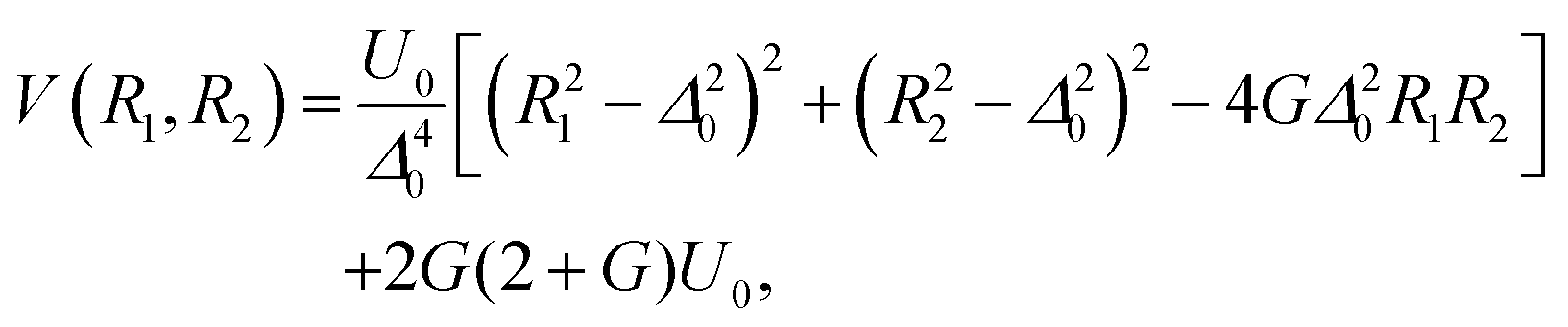 | (8) |
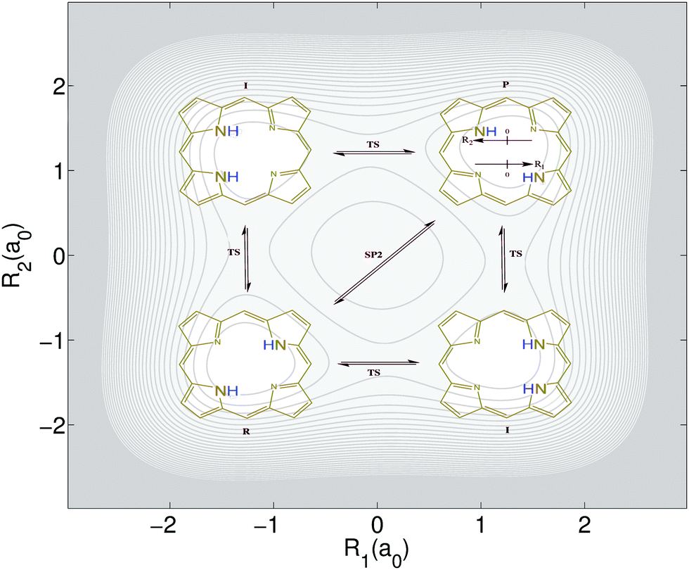 | ||
| Fig. 1 Double proton tranfer of the model porphine. The protons move along coordinates R1 and R2. The four snapshots represent the transfer of the two protons from reactant (R) to product (P), sequentially along intermediate states (I) involving four transition states (TS), or simultaneously through a second order saddle point (SP2). In the background: Potential energy surface for the model porphine, eqn (8), adopted from ref. 41–43. The equidistant values of the contours range from 0 eV, for the potential minima of the reactant (R) and product (P) configurations, to 5 eV. The corresponding energies of the local minima for the intermediates (I), of the four barriers labeled TS, and of the second order saddle point (SP2) are 0.238, 0.600, and 1.069 eV, respectively. | ||
The model potential in eqn (8) is symmetric with respect to the diagonals R1 = ±R2. It accommodates nearly degenerate doublets of eigenstates Ψv+(R1,R2) and Ψv−(R1,R2), with energies below the barriers TS, plus higher excited states. We then chose our initial state to be of the general form:
| Ψ0(R1,R2;ΔR) = Ψ0,R(R1 + ΔR,R2 + ΔR), | (9) |
 is a superposition state that represents the localized ground state wavefunction of the reactant, with Ψ0+(R1,R2) and Ψ0−(R1,R2) representing the lowest doublet (ν = 0), i.e., HΨν±(R1,R2) = Eν±Ψν±(R1,R2), where H is the full Hamiltonian of the system, i.e.:
| H(R1,R2) = TR1 + TR2 + V(R1,R2), | (10) |
 the kinetic energies of the two protons, M = mp the proton mass, and V(R1,R2) the scalar potential given in eqn (8).
Due to the symmetry of the model potential in eqn (8), the localized ground state wavefunction of the reactant is equivalent to the localized ground state wavefunction of the product. Therefore, the initial states in eqn (9) are, in fact, representative of two equivalent configurations where the two protons are placed along the reactant–product diagonal (see Fig. 2).
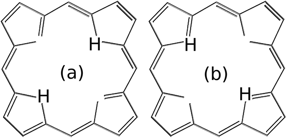 | ||
| Fig. 2 Due to the symmetry of the model potential used in this work, i.e., eqn (8), the states in eqn (9) are representative of the two equivalent hydrogen configurations in (a) and (b). | ||
The localization, eqn (9), of the reactant wavefunction may be generated by symmetry breaking, for example, by selective deuteration of the C4N rings for the reactant; this would not change the PES, but it would induce localization of the reactant wavefunction due to the slightly heavier mass that is associated with the reactant compared to the product.42 Also, shifts of initial wavefunctions from equilibrium to non-equilibrium positions may be induced, for example, by means of pump–dump laser pulse control,48 as designed by Tannor and Rice.49–51 Essentially, the ultrashort pump pulse transfers the molecule from the electronic ground state to an excited state. Here, the system evolves from the original configuration until it is shifted to the target position. Finally, the dump pulse brings the wavepacket back to the electronic ground state, thus preparing the initial state for the subsequent reaction. Analogous shifts of the original wavefunctions to nonequilibrium positions have been demonstrated by means of laser pulse control, by Kapteyn, Murnane, and co-workers.52
4 Equilibration time
To gain some insight into the behaviour of the effective dimension and the equilibration time in porphine, we consider the case of initial states defined in eqn (9) and the type of projective position measurements:![[R with combining circumflex]](https://www.rsc.org/images/entities/i_char_0052_0302.gif) = |R1〉〈R1| ⊗ = |R1〉〈R1| ⊗ ![[Doublestruck I]](https://www.rsc.org/images/entities/char_e16c.gif) 2 + 1 ⊗ |R2〉〈R2|. 2 + 1 ⊗ |R2〉〈R2|. | (11) |
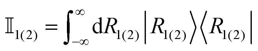 are identity operators in the position representation acting, respectively, in the subspaces defined by R1 and R2. Whereas the position operator in eqn (11) involves an infinite Hilbert space, the relevant energy subspace is finite in practice (for numerical purposes) and hence it is possible to apply the machinery introduced above.
We evaluate the effective dimension deff in eqn (5) and the equilibration time Teq in (6) for different values of ΔR ∈ [−2.7,2.7] (see Fig. 3). For that, we first computed vα = cj*Rjici/σR, where Rij := 〈Ei||Ej〉 and σR = Rmax − Rmin has been chosen to be σR = 3σgs, and  is the dispersion of the localized ground state wavefunction of the reactant.
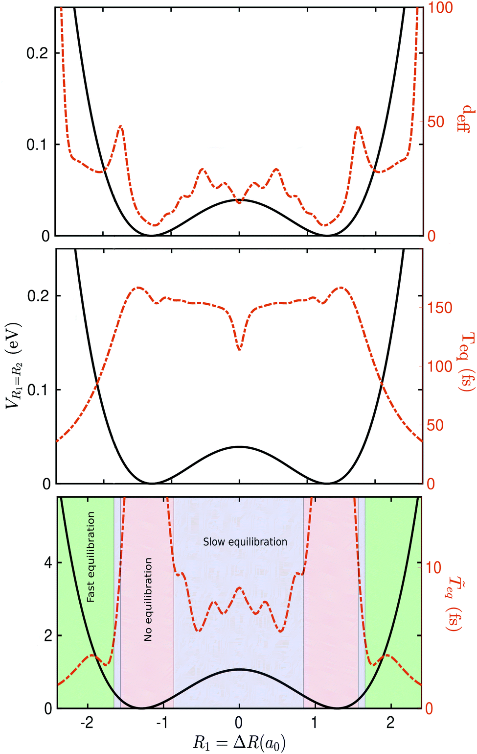 | ||
Fig. 3 Effective dimension deff (top panel), equilibration time Teq (mid panel), and effective equilibration time ![[T with combining tilde]](https://www.rsc.org/images/entities/i_char_0054_0303.gif) (bottom panel), all in dashed red line. The results are for the initial states defined in eqn (9) and different values of ΔR for the type of measurement defined in eqn (11) using a square grid of size 151a0 with a grid spacing of 0.08a0. The Born–Oppenheimer potential-energy surface is also plot in solid black line for reference. Three different regions are identified in the bottom panel: (i) in green, regions where equilibration is expected to occur rapidly, (ii) in blue, regions where equilibration is expected to be attained slowly, and (iii) in red, regions where equilibration is not expected to occur. (bottom panel), all in dashed red line. The results are for the initial states defined in eqn (9) and different values of ΔR for the type of measurement defined in eqn (11) using a square grid of size 151a0 with a grid spacing of 0.08a0. The Born–Oppenheimer potential-energy surface is also plot in solid black line for reference. Three different regions are identified in the bottom panel: (i) in green, regions where equilibration is expected to occur rapidly, (ii) in blue, regions where equilibration is expected to be attained slowly, and (iii) in red, regions where equilibration is not expected to occur. | ||
In addition to deff, which represents an equilibration criterion, and Teq, which provides an estimate of the velocity of the equilibration process, we found convenient to show also these two concepts in a compact way by introducing an effective equilibration time (or effective equilibration speed):
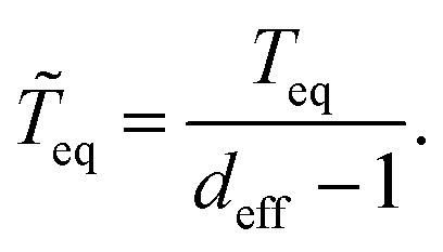 | (12) |
eq can still be close to infinite for initial states being eigenstates of the observable of interest (i.e., deff ∼ 1).
The resulting values of deff, Teq and eq are plotted in Fig. 3. We identified three different regions: (i) in green, regions where equilibration is expected to occur fast, (ii) in blue, regions where equilibration is expected to occur slowly, and (iii) in red, regions where equilibration is not expected to occur. Interestingly, region (iii) corresponds to the regime where our initial state can be written as the superposition of a very small number of energy eigenstates. Note that for ΔR ≈ 0 then Ψ0 is just the sum of two energy eigenstates Ψ0+ and Ψ0−. The number of energy eigenstates required to define the initial wavefunction increases as one departs from the global minima. Regions of slow equilibration (in blue) are the result of a non-trivial interplay between Teq and deff. Note, for example, the relative minimum shown by Teq at ΔR = 0 that corresponds to the situation where the initial wavefunction would fall equally to the left and right wells. In regions where equilibration is expected to occur fast (in green), the equilibration time Teq decreases almost monotonically. This is due to the fact that the barrier leads to a very effective dephasing mechanism at energies close or above the global maximum.
It is important to emphasize that the quantities deff, Teq and eq are to be understood only as qualitative descriptors of equilibration, as they are defined using rather heuristic arguments. Therefore, as it will be shown in the next section, these quantities do not provide an accurate quantitative estimation of the equilibration time, but do provide us with a good guess.
5 Equilibration dynamics
We now aim to study the dynamics that leads to equilibration for initial states induced by pump–dump laser pulse control of the form in eqn (9). Specifically, we choose ΔR = −2.2a0 such that the initial state lies in the rapid equilibration regime (see Fig. 3). The mean energy of this initial state is rather high (4.885 eV) and well above the TS and SP2 barriers (respectively 0.600 eV and 1.069 eV).Starting with Ψ0(R1,R2;−2.2a0) (see Fig. 4a), the initial synchronous mechanism of the first forward reaction is characterized by a rapid dispersion of the wavepacket and relief reflections of the broadened wavepacket from wide regions of the steep repulsive wall of the PES close to the minimum of the product that leads to the switch from the sequential to the synchronous mechanism (see Fig. 4b). This situation is reminiscent of the near field interference effect arising when periodic diffracting structures are illuminated by highly coherent light or particle beams.53
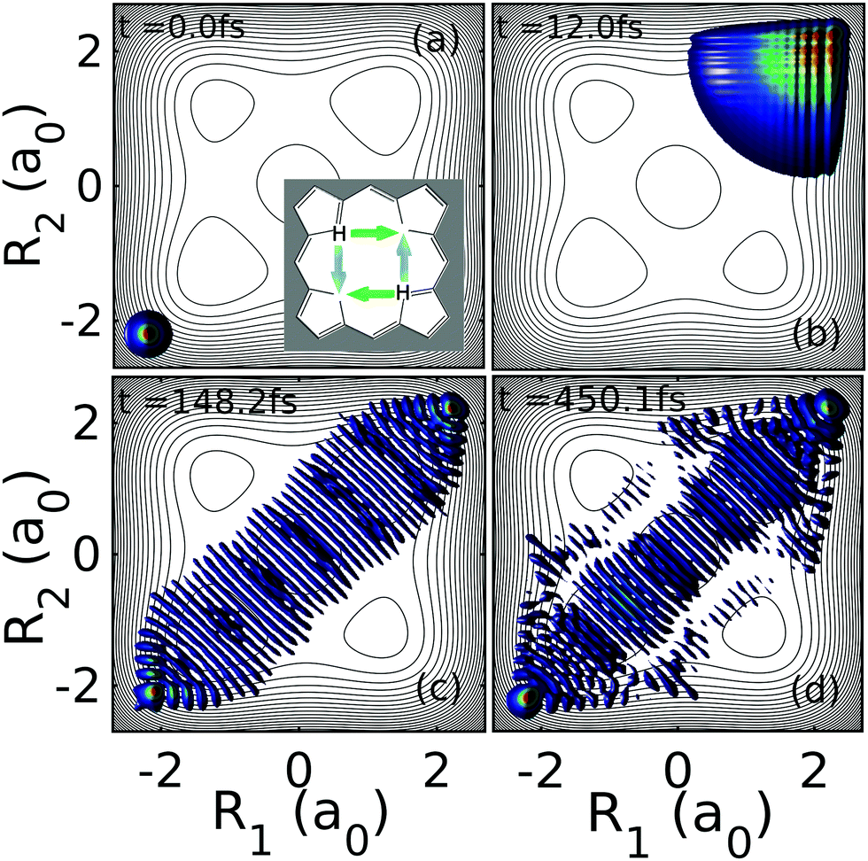 | ||
| Fig. 4 Dynamics of the two-proton density |Ψ(R1,R2,t)|2 at four different time snapshots for the initial state Ψ0(R1,R2;−2.2a0). The initially well-localized nuclear density gives way later to a strong proton delocalization along the synchronous pathway that is maintained for at least 1 ps. | ||
The time dilation supported by continuous wavepacket dispersion leads to a strong proton delocalization. An apparently “chaotic” flux is however coherently directing the recovery of the concerted double proton transfer at t ≳ 100 fs. Due to the dephasing between partial waves, the grid structure of the probability density associated to the sequential double proton transfer progressively dilutes into what is reminiscent of a stationary state, showing a series of minima disposed perpendicular to the diagonal R1 = R2 (see Fig. 4c). The long-lived quasi-stationary state, formed already at ∼150 fs, lasts beyond 500 fs (see Fig. 4d) and it gives rise to the equilibration of the position operator in eqn (11) as well as of the momentum operator ![[P with combining circumflex]](https://www.rsc.org/images/entities/i_char_0050_0302.gif) = |P1〉〈P1| ⊗ 2 + 1 ⊗ |P2〉〈P2|. The full evolution dynamics can be found in S1 (ESI†).
= |P1〉〈P1| ⊗ 2 + 1 ⊗ |P2〉〈P2|. The full evolution dynamics can be found in S1 (ESI†).
The above dynamics result into an effective equilibration of the phase-space variables. In Fig. 5 (top panel) we show the differences ![[R with combining macron]](https://www.rsc.org/images/entities/i_char_0052_0304.gif) − 〈(t)〉 and
− 〈(t)〉 and ![[P with combining macron]](https://www.rsc.org/images/entities/i_char_0050_0304.gif) − 〈(t)〉 as a function of time for the initial state Ψ0(R1,R2;−2.2a0). Equilibration is achieved once these differences become small (≪1) and stay small for a lapse of time that is comparable to the relevant time-scale of the dynamics.54
− 〈(t)〉 as a function of time for the initial state Ψ0(R1,R2;−2.2a0). Equilibration is achieved once these differences become small (≪1) and stay small for a lapse of time that is comparable to the relevant time-scale of the dynamics.54
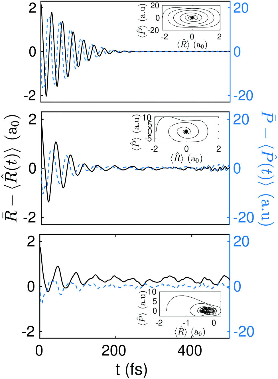 | ||
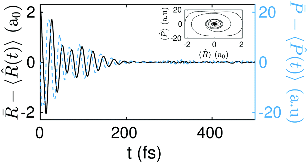
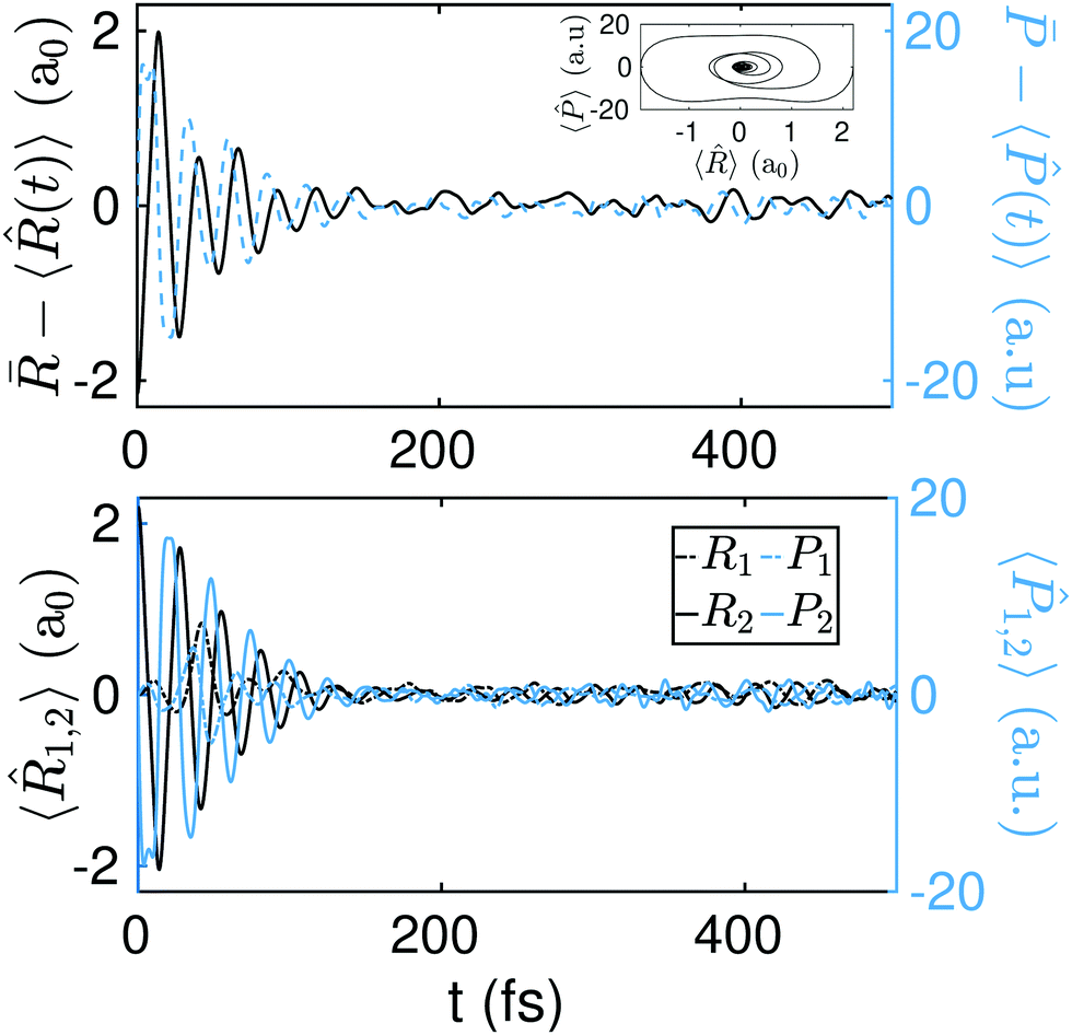
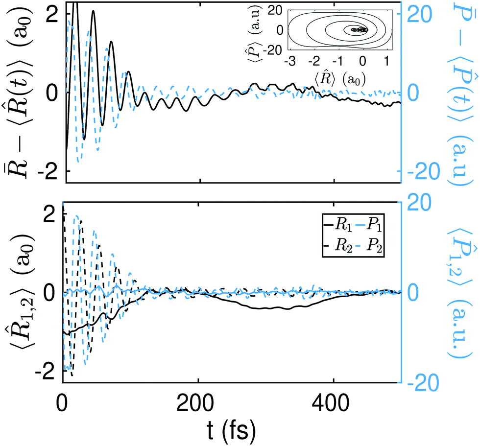
| Fig. 5 Equilibration of the position (solid black line) and momentum (dashed blue line). In the inset: Ensemble average of the phase space as a function of time. Upper panel: The initial state, Ψ0(R1,R2;−2.2a0), has an energy of 4.885 eV, i.e., 3.7 eV above the SP2. Middle panel: The initial state, Ψ0(R1,R2;−1.9a0), has an energy of 1.905 eV, i.e., 0.8 eV above the SP2. Bottom panel: The initial state, Ψ0(R1,R2;−1.75a0), has an energy of 1.185 eV, i.e., 0.1 eV above the SP2. The values of deff, Teff, and eff for the three different initial conditions ΔR(a0) = {−2.2,−1.9,−1.75}, are respectively deff = {29.89,33.39,48.2}, Teq = {35.12 fs,59.27 fs,72.75 fs}, and eq = {1.17 fs,1.77 fs,1.51 fs}. | ||
The equilibration of the position and momentum yields a phase-space portrait (see the inset in Fig. 5 top panel) that is reminiscent of the phase-space portrait of a damped harmonic oscillator. Interestingly, this phase-space dynamics is attained here without any loss (nor gain) of energy.
In Fig. 5 (middle and bottom panels) we show the dynamics of − 〈(t)〉 and − 〈(t)〉 for another two different initial states, viz., Ψ0(R1,R2;−1.9a0) and Ψ0(R1,R2;−1.75a0), with energies 1.905 eV and 1.185 eV (i.e., ∼0.8 eV and ∼0.1 eV above the SP2 barrier) respectively. As we decrease ΔR and thus approach the equilibrium position ΔR = 0, the energy of the initial state gets closer to the top of the synchronous barrier. This results into a dynamics that departs more and more from an equilibration process. Note, for instance, that while the phase-space portrait in Fig. 5 (mid panel) is still reminiscent of some damped dynamics, the phase-space diagram in Fig. 5 (bottom panel) is clearly not, as it does not converge to equilibrium. For even smaller ΔR values, the initial states fall down into the minimum of the well, where equilibration is no longer expected to occur. The full dynamics for the initial states Ψ0(R1,R2;−2.2a0), Ψ0(R1,R2;−1.9a0), and Ψ0(R1,R2;−1.75a0) can be found in S1, S2, and S3 (ESI†) respectively.
6 Discussion
One might think that provided there are at least two degrees of freedom with non-negligible coupling between each other, one can expect one to act as a bath for the other and vice versa, both leading to the damping of the mutual dynamics. As a result, one may encounter that observables reach some equilibrium value. While this hypothesis might sound reasonable, it is incorrect. First of all, two particles with identical masses (e.g., two protons) can hardly act one as a bath for the other. Second, even a system with a single degree of freedom can equilibrate. See for example the works in ref. 54 and 55. In order a quantum system to equilibrate there is no need for a bath. That is the main point that differentiates equilibration from thermalization. Also, working with initial conditions far-from-equilibrium within anharmonic regions of the potential-energy surface does not guarantee equilibration. Otherwise equilibration should be observed for almost every molecule out-of-equilibrium. This is definitely not the case.To gain more insight into the physical mechanism that yields equilibration, we here take advantage of the interpretation value of Bohmian mechanics.56–61 It is possible to reinterpret the quantum formalism as describing particles following definite trajectories, each with a precisely defined position at each instant in time. In this interpretation, called Bohmian mechanics, the trajectories of the particles are guided by the wavefunction. This allows for phenomena such as double-slit interference, as has been investigated experimentally for single photons.62–64 Note that this is different from semi-classical trajectories,65–67 other generalized hydrodynamic approaches,68 and also from the Feynman path formalism of quantum mechanics.69 For example, in contrast to the Feynman formalism, Bohmian mechanics says that each quantum particle in a given experiment follows a trajectory in a deterministic manner. Thus, much of the intuition of classical mechanics is regained.70 In any case, let us insist that we use an ensemble of exact Bohmian trajectories (evaluated from the wavefunction solution of the time-dependent Schrödinger equation) with the only intention to provide a different viewpoint on the process of equilibration that is more “digestible” for an adherent of classical mechanics and that it is at the same time compatible with the expectation values associated to the exact quantum dynamics.
We consider an ensemble of Bohmian trajectories {Rα(t)} = {Rα1(t),Rα2(t)} initially sampled from the probability distribution P(R1,R2) = |Ψ0(R1,R2,−2.2a0)|2 and whose time evolution is defined as
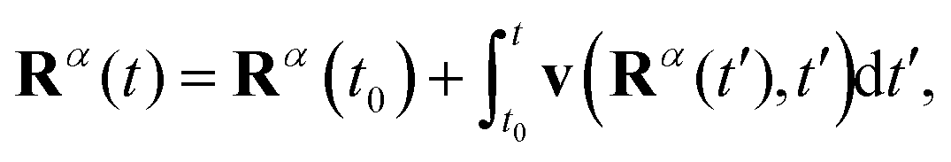 | (13) |
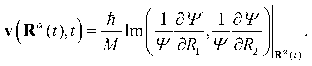 | (14) |
In Fig. 6 we show the time evolution of an ensemble of five hundred Bohmian trajectories Rα1(t) sampled from |Ψ0(R1,R2,−2.2a0)|2. An initially orchestrated oscillatory dynamics with an amplitude that extends over the two wells is rapidly (at around ∼50 fs) substituted by apparently incoherent oscillations with a very small amplitude. Not much later, at around 150 fs, the trajectories fall into a dynamics that is highly localized and homogeneously distributed. Of particular interest is the fine structure of the Bohmian trajectories, characterized by high frequency components and rapid shifts in their direction. This quantum mechanical motion arises from strong time-dependent quantum force fields (originating from quantum interferences) which essentially dominate the dynamics and are responsible for shifting the direction of trajectories away from that dictated by the classical force field.
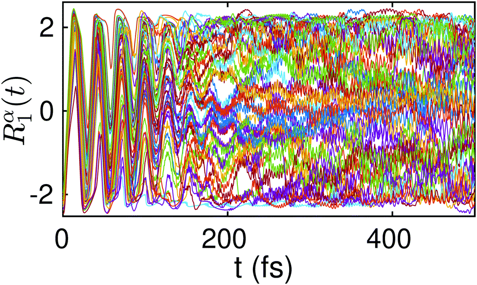 | ||
| Fig. 6 Time evolution of a randomly chosen set of five hundred Bohmian trajectories Rα1(t) sampled from |Ψ0(R1,R2,−2.2a0)|2. | ||
As already anticipated in Section (4), the above dynamics can be seen as the result of a very efficient dephasing mechanism that leads to a diagonal ensemble. The barrier in between the two wells induces a continuous time dilatation supported by wavepacket dispersion that yields strong interference effects between different parts of the wavepacket. Eventually, these interferences are responsible for freezing the transfer of the two protons and lead to the localization of the corresponding trajectories within the concerted pathway (see Fig. 6). This equilibration dynamics corresponds to the picture where the two protons become localized at certain configurations along the concerted transfer reaction path, as if they were associated to a stationary state.
In view of the above results, we may conclude that there are two effects that must coexist to find equilibration:
(i) Initial states consisting of a large superposition of energy eigenstates.
(ii) The presence of a very effective dephasing mechanism.
Note that these two conditions are not easily met in general, but can be found for the porphine molecule and probably also for other related molecules, under certain initial conditions. More specifically, for the porphine model considered in this work, condition (i) is met for initial states with energies well above the SP2 barrier, and the dephasing mechanism in condition (ii) is originated by the SP2 barrier.
Concerning condition (i), there are other types of initial states, different from those defined in eqn (9), that can be considered as potentially leading to the equilibration of the canonical variables and . Very general initial conditions can be defined, for example, by introducing the wavefunction ΨG(R1 + ΔR1,R2 + ΔR2), where ΨG(R1,R2) represents a Gaussian approximation to the localized ground state wavefunction of the reactant, with a dispersion  and centered at the origin of coordinates. In particular, for ΔR1 = −ΔR2, the wavepacket ΨG(R1 + ΔR1,R2 + ΔR2) is centered along the diagonal R1 = −R2 that leads from one Intermediate to the other (i.e., perpendicular to the diagonal R1 = R2 that leads from the reactant to the product). Due to the symmetry of the model potential in eqn (8), the state ΨG(R1 + ΔR1,R2 − ΔR1) around the Intermediate minima, may correspond to four equivalent hydrogen atoms distributions (see Fig. 7). Starting from the initial state ΨG(R1 + 2.2a0,R2 − 2.2a0), the resulting dynamics is analogous to that shown in Fig. 4 but the probability density that corresponds to Fig. 4c and d extends now along the diagonal R1 = −R2 instead of R1 = R2 and there is a notable increase of the probability density along the sequential paths. The associated behaviour of 〈〉 and 〈〉 is not significantly different from the results in Fig. 5. Specifically, the results in Fig. 8 illustrate that the present definition of “quantum equilibration” in eqn (1) allows relaxation to states that are far from the traditional equilibrium scenarios, which are centered close to the potential minima. The full dynamics for the initial state ΨG(R1 + 2.2a0,R2 − 2.2a0) can be found in S4 (ESI†).
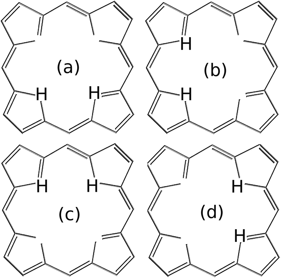 | ||
| Fig. 7 Due to the symmetry of the model potential defined in eqn (8), the initial states ΨG(R1 + ΔR1,R2 − ΔR1) localized around the intermediate minima may correspond to the four equivalent proton distributions in (a–d). | ||
 | ||
| Fig. 8 Equilibration of the position (solid black line) and momentum (dashed blue line) for the initial state ΨG(R1 + 2.2a0,R2 − 2.2a0). In the inset: Ensemble average of the phase space as a function of time. The initial state, ΨG(R1 + 2.2a0,R2 − 2.2a0), has an energy of 5.10 eV, i.e., 4.03 eV above the SP2. | ||
Other initial states, with resulting dynamics occurring outside the two main diagonals (concerted mechanism of proton transfer), can be also considered. Should the wavepacket be displaced along only one degree of freedom, one would likely observe the sequential mechanism of the proton transfer. In Fig. 9 and 10, we show the dynamics of 〈〉 and 〈〉 (and the corresponding expectation value dynamics of 〈1,2〉 and 〈1,2〉) that result from the initial states ΨG(R1 + 2.2a0,R2) and ΨG(R1 + 2.2a0,R2 − 1.0a0) respectively. The full dynamics for the initial states ΨG(R1 + 2.2a0,R2) and ΨG(R1 + 2.2a0,R2 − 1.0a0) can be found respectively in S5 and S6 (ESI†).
 | ||
| Fig. 9 Top panel: Equilibration of the position (solid black line) and momentum (dashed blue line) for the initial state ΨG(R1 + 2.2a0,R2). In the inset: Ensemble average of the phase space as a function of time. The initial state, ΨG(R1 + 2.2a0,R2), has an energy of 3.08 eV, i.e., 2.01 eV above the SP2. Bottom panel: Dynamics of 〈1,2〉 and 〈1,2〉. | ||
 | ||
| Fig. 10 Top panel: Equilibration of the position (solid black line) and momentum (dashed blue line) for the initial state ΨG(R1 + 2.2a0,R2 − 1.0a0). In the inset: Ensemble average of the phase space as a function of time. The initial state, ΨG(R1 + 2.2a0,R2 − 1.0a0), has an energy of 2.85 eV, i.e., 1.78 eV above the SP2. Bottom panel: Dynamics of 〈1,2〉 and 〈1,2〉. | ||
As it is apparent from all the above dynamics, the symmetry of the initial state does not seem to play a crucial role. Instead, it seems to be the energy of the initial state in comparison with the height of the SP2 barrier what determines whether or not equilibration will take place. As the energy of the initial wavepacket is decreased and gets closer to the height of the SP2 barrier, it takes longer to equilibrate. Overall, this is in consonance with the theoretical predictions in Fig. 3.
In general, our results are in accordance with the idea that the diagonal and microcanonical ensembles give the same predictions for the relaxed value,29i.e.:
 | (15) |
7 Conclusions
To summarize, we have shown that quantum equilibration, mostly studied for many-body systems made of a large number of particles, can also play a role in isolated molecular systems that involve a few number of degrees of freedom. Specifically, we have seen that a two-dimensional model system describing the double proton transfer in porphine can present equilibration dynamics for a wide range of far-from-equilibrium initial states that are compatible with a pump–dump preparation scheme. We have seen that the resulting equilibration state is reached in ∼200 fs and that it is associated with zero mean position and momentum of the two protons. This equilibration state is characterized by a strong delocalization of the probability density of the protons, which can appear either along the concerted or sequential transfer paths depending on the symmetry of the initial conditions.By picking up a number of very general initial conditions, we have shown that the symmetry of the initial state does not play a crucial role. Instead, it is the energy of the initial state in comparison with the height of the SP2 barrier what determines whether or not equilibration will take place and how long it will take to develop. We have thus concluded that there are two main facts that must coexist to find equilibration:40 (i) initial states consisting of a large superposition of energy eigenstates, and (ii) the presence of a very effective dephasing mechanism. For the porphine model considered in this work, condition (i) is met for initial states with energies well above the SP2 barrier, and it is the SP2 barrier itself that facilitates the fulfillment of (ii). This conclusion is compatible with the idea that the diagonal and microcanonical ensembles give the same predictions for the relaxed value for a wide range of initial conditions.29
Relying on the de Broglie–Bohm interpretation of quantum mechanics, we have shown that the equilibration process in porphine can be associated with the picture where, due to strong interferences, the two protons become localized at certain configurations along the concerted and sequential transfer paths as if they where associated to a stationary state. This result may help, for example, in the interpretation of experimental data. That is, the close connection between Bohmian mechanics and weak values64,71,72 provides an operational interpretation of the above described equilibration mechanism based on trajectories that could be put within reach of experimental verification.62,63 Let us insist that Bohmian trajectories have been introduced in this work with the intention to gain insight into the physical mechanism that yields equilibration. However, the conclusion that equilibration is actually taking place is based solely on the analysis of the time-evolution of the position and momentum expectation values (which are not dependent on the particular interpretation choice).
Witnessing equilibration dynamics in the laboratory for an arbitrary type of molecules could be feasible thanks to the development of femtosecond spectroscopy73,74 and to the most recent technological advances that allow characterizing wavepacket dynamics at an experimental level in a wide variety of molecular systems.75–77 However, whether quantum equilibration dynamics in an isolated porphine molecule might be actually observed will strongly depend on the validity of the approximations considered in the employed model. The model porphine considered here does not include the effect of the heavy atom vibrations of the molecular scaffold,78 and therefore, while it served well for a proof of principle, the excitation of specific heavy atom vibrations might have a sizable influence on the proton transfer dynamics. Yet, avoiding possible effects coming from the scaffold dynamics could be possible. Because of the bistability in the position of the two protons, which can occupy different, energetically equivalent positions (tautomerization), porphines have been devised as molecular switches.79–82 In this respect, there exist an extensive literature (see e.g.ref. 80) on the control of the scaffold structural freedom by means of surface anchoring81,83 or molecular assembling.82,84
Finally, let us mention a recent work where the third law of thermodynamics is investigated for a 1D model boron rotor B13+.55 In ref. 55 the entropy production reaches a stationary (or quasi-stationary) value (3.017). This value, however, does not correspond to the equilibrium value (3.401), which is far beyond the variance of the fluctuations (0.101). In the authors words: “this points to incomplete equilibration”. Furthermore, this quasi-equilibration process occurs in approximately 10 picoseconds. At the time scale of a few picoseconds it is difficult to imagine that the coupling of the rotation/pseudo-rotation of the boron rotor to the rest of degrees of freedom will not modify the dynamics.
Conflicts of interest
There are no conflicts to declare.Acknowledgements
The authors acknowledge financial support from the Spanish Ministerio de Economía y Competitividad (Projects No. CTQ2016-76423-P and No. PID2019-109518GB-I00), the Generalitat de Catalunya (Project No. 2017 SGR 348), and the Spanish Structures of Excellence María de Maeztu program (through grant MDM-2017-0767). G. A. acknowledges also financial support from the European Union Horizon 2020 research and innovation programme under the Marie Sklodowska-Curie Grant Agreement No. 752822. Open Access funding provided by the Max Planck Society.Notes and references
- C. Gogolin and J. Eisert, Rep. Prog. Phys., 2016, 79, 056001 CrossRef.
- P. Reimann, Phys. Rev. Lett., 2007, 99, 160404 CrossRef.
- S. Goldstein, J. L. Lebowitz, R. Tumulka and N. Zangh, Phys. Rev. Lett., 2006, 96, 050403 CrossRef.
- S. Popescu, A. J. Short and A. Winter, Nat. Phys., 2006, 2, 754 Search PubMed.
- P. Reimann, Phys. Rev. Lett., 2008, 101, 190403 CrossRef.
- N. Linden, S. Popescu, A. J. Short and A. Winter, Phys. Rev. E: Stat., Nonlinear, Soft Matter Phys., 2009, 79, 061103 CrossRef.
- M. Greiner, O. Mandel, T. W. Hänsch and I. Bloch, Nature, 2002, 419, 51 CrossRef CAS.
- M. Greiner, O. Mandel, T. Esslinger, T. W. Hänsch and I. Bloch, Nature, 2002, 415, 39 CrossRef CAS.
- A. Tuchman, C. Orzel, A. Polkovnikov and M. Kasevich, Phys. Rev. A: At., Mol., Opt. Phys., 2006, 74, 051601 CrossRef.
- I. Bloch, Nat. Phys., 2005, 1, 23 Search PubMed.
- T. Langen, R. Geiger and J. Schmiedmayer, Annu. Rev. Condens. Matter Phys., 2015, 6, 201–217 Search PubMed.
- L. Sadler, J. Higbie, S. Leslie, M. Vengalattore and D. Stamper-Kurn, Nature, 2006, 443, 312 CrossRef CAS.
- T. Kinoshita, T. Wenger and D. S. Weiss, Nature, 2006, 440, 900 CrossRef CAS.
- S. Hofferberth, I. Lesanovsky, B. Fischer, T. Schumm and J. Schmiedmayer, Nature, 2007, 449, 324 CrossRef CAS.
- A. Weller, J. Ronzheimer, C. Gross, J. Esteve, M. Oberthaler, D. Frantzeskakis, G. Theocharis and P. Kevrekidis, Phys. Rev. Lett., 2008, 101, 130401 CrossRef CAS.
- D. Porras and J. I. Cirac, Phys. Rev. Lett., 2004, 92, 207901 CrossRef CAS.
- A. Friedenauer, H. Schmitz, J. T. Glueckert, D. Porras and T. Schätz, Nat. Phys., 2008, 4, 757 Search PubMed.
- H. Häffner, W. Hänsel, C. Roos, J. Benhelm, M. Chwalla, T. Körber, U. Rapol, M. Riebe, P. Schmidt and C. Becher, Nature, 2005, 438, 643 CrossRef.
- P. Jurcevic, B. P. Lanyon, P. Hauke, C. Hempel, P. Zoller, R. Blatt and C. F. Roos, Nature, 2014, 511, 202 CrossRef CAS.
- B. P. Lanyon, C. Hempel, D. Nigg, M. Müller, R. Gerritsma, F. Zähringer, P. Schindler, J. T. Barreiro, M. Rambach and G. Kirchmair, Science, 2011, 334, 57–61 CrossRef CAS.
- P. Schindler, M. Müller, D. Nigg, J. T. Barreiro, E. A. Martinez, M. Hennrich, T. Monz, S. Diehl, P. Zoller and R. Blatt, Nat. Phys., 2013, 9, 361 Search PubMed.
- R. Blatt and C. F. Roos, Nat. Phys., 2012, 8, 277 Search PubMed.
- J. W. Britton, B. C. Sawyer, A. C. Keith, C.-C. J. Wang, J. K. Freericks, H. Uys, M. J. Biercuk and J. J. Bollinger, Nature, 2012, 484, 489 CrossRef CAS.
- S. Trotzky, Y.-A. Chen, A. Flesch, I. P. McCulloch, U. Schollwöck, J. Eisert and I. Bloch, Nat. Phys., 2012, 8, 325 Search PubMed.
- M. Cheneau, P. Barmettler, D. Poletti, M. Endres, P. Schauß, T. Fukuhara, C. Gross, I. Bloch, C. Kollath and S. Kuhr, Nature, 2012, 481, 484 CrossRef CAS.
- T. Langen, R. Geiger, M. Kuhnert, B. Rauer and J. Schmiedmayer, Nat. Phys., 2013, 9, 640 Search PubMed.
- M. Gring, M. Kuhnert, T. Langen, T. Kitagawa, B. Rauer, M. Schreitl, I. Mazets, D. A. Smith, E. Demler and J. Schmiedmayer, Science, 2012, 337, 1318–1322 CrossRef CAS.
- J. P. Ronzheimer, M. Schreiber, S. Braun, S. S. Hodgman, S. Langer, I. P. McCulloch, F. Heidrich-Meisner, I. Bloch and U. Schneider, Phys. Rev. Lett., 2013, 110, 205301 CrossRef CAS.
- M. Rigol, V. Dunjko and M. Olshanii, Nature, 2008, 452, 854 CrossRef CAS.
- M. Rigol, Phys. Rev. Lett., 2009, 103, 100403 CrossRef.
- M. Moeckel and S. Kehrein, Phys. Rev. Lett., 2008, 100, 175702 CrossRef.
- C. Kollath, A. M. Läuchli and E. Altman, Phys. Rev. Lett., 2007, 98, 180601 CrossRef.
- S. Deng, G. Ortiz and L. Viola, Phys. Rev. B: Condens. Matter Mater. Phys., 2011, 83, 094304 CrossRef.
- L. C. Venuti and P. Zanardi, Phys. Rev. A: At., Mol., Opt. Phys., 2010, 81, 032113 CrossRef.
- F. Goth and F. F. Assaad, Phys. Rev. B: Condens. Matter Mater. Phys., 2012, 85, 085129 CrossRef.
- M. Rigol and M. Fitzpatrick, Phys. Rev. A: At., Mol., Opt. Phys., 2011, 84, 033640 CrossRef.
- E. Torres-Herrera and L. F. Santos, Phys. Rev. A: At., Mol., Opt. Phys., 2014, 89, 043620 CrossRef.
- A. J. Short, New J. Phys., 2011, 13, 053009 CrossRef.
- A. J. Short and T. C. Farrelly, New J. Phys., 2012, 14, 013063 CrossRef.
- T. R. de Oliveira, C. Charalambous, D. Jonathan, M. Lewenstein and A. Riera, New J. Phys., 2018, 20, 033032 CrossRef.
- Z. Smedarchina, W. Siebrand and A. Fernández-Ramos, J. Chem. Phys., 2007, 127, 174513 CrossRef.
- A. Accardi, I. Barth, O. Kühn and J. Manz, J. Phys. Chem. A, 2010, 114, 11252–11262 CrossRef CAS.
- G. Albareda, J. M. Bofill, I. Tavernelli, F. Huarte-Larrañaga, F. Illas and A. Rubio, J. Phys. Chem. Lett., 2015, 6, 1529–1535 CrossRef CAS.
- T. J. Butenhoff and C. B. Moore, J. Am. Chem. Soc., 1988, 110, 8336–8341 CrossRef CAS.
- J. Braun, M. Koecher, M. Schlabach, B. Wehrle, H.-H. Limbach and E. Vogel, J. Am. Chem. Soc., 1994, 116, 6593–6604 CrossRef CAS.
- J. Braun, H.-H. Limbach, P. G. Williams, H. Morimoto and D. E. Wemmer, J. Am. Chem. Soc., 1996, 118, 7231–7232 CrossRef CAS.
- Z. Smedarchina, M. Z. Zgierski, W. Siebrand and P. M. Kozlowski, J. Chem. Phys., 1998, 109, 1014–1024 CrossRef CAS.
- M. K. Abdel-Latif and O. Kühn, Theor. Chem. Acc., 2011, 128, 307–316 Search PubMed.
- D. J. Tannor and S. A. Rice, J. Chem. Phys., 1985, 83, 5013–5018 CrossRef CAS.
- D. J. Tannor, R. Kosloff and S. A. Rice, J. Chem. Phys., 1986, 85, 5805–5820 CrossRef CAS.
- M. Shapiro and P. Brumer, Quantum Control of Molecular Processes, John Wiley & Sons, 2012 Search PubMed.
- W. Li, X. Zhou, R. Lock, S. Patchkovskii, A. Stolow, H. C. Kapteyn and M. M. Murnane, Science, 2008, 322, 1207–1211 CrossRef CAS.
- A. S. Sanz and S. Miret-Artés, J. Chem. Phys., 2007, 126, 234106 CrossRef CAS.
- A. S. Malabarba, N. Linden and A. J. Short, Phys. Rev. E: Stat., Nonlinear, Soft Matter Phys., 2015, 92, 062128 CrossRef.
- D. Jia, J. Manz and Y. Yang, AIP Adv., 2018, 8, 045222 CrossRef.
- A. Benseny, G. Albareda, Ã. S. Sanz, J. Mompart and X. Oriols, Eur. Phys. J. D, 2014, 68, 1–42 CrossRef CAS.
- X. Oriols and J. Mompart, Applied Bohmian Mechanics: From Nanoscale Systems to Cosmology, Pan Stanford, Florida, USA, 2012 Search PubMed.
- G. Albareda, H. Appel, I. Franco, A. Abedi and A. Rubio, Phys. Rev. Lett., 2014, 113, 083003 CrossRef.
- G. Albareda, A. Abedi, I. Tavernelli and A. Rubio, Phys. Rev. A, 2016, 94, 062511 CrossRef.
- L. González and R. Lindh, Quantum Chemistry and Dynamics of Excited States: Methods and Applications, Wiley, 2020 Search PubMed.
- G. Albareda, A. Kelly and A. Rubio, Phys. Rev. Mater., 2019, 3, 023803 CrossRef CAS.
- S. Kocsis, B. Braverman, S. Ravets, M. J. Stevens, R. P. Mirin, L. K. Shalm and A. M. Steinberg, Science, 2011, 332, 1170–1173 CrossRef CAS.
- D. H. Mahler, L. Rozema, K. Fisher, L. Vermeyden, K. J. Resch, H. M. Wiseman and A. Steinberg, Sci. Adv., 2016, 2, e1501466 CrossRef.
- F. Traversa, G. Albareda, M. Di Ventra and X. Oriols, Phys. Rev. A: At., Mol., Opt. Phys., 2013, 87, 052124 CrossRef.
- W. H. Miller, Faraday Discuss. Chem. Soc., 1977, 62, 40–46 RSC.
- G. Albareda, X. Saura, X. Oriols and J. Suné, J. Appl. Phys., 2010, 108, 043706 CrossRef.
- Y. Goldfarb, J. Schiff and D. J. Tannor, J. Chem. Phys., 2008, 128, 164114 CrossRef.
- B. Doyon, 2019, arXiv preprint arXiv:1912.08496.
- R. P. Feynman, Feynman's Thesis – A New Approach to Quantum Theory, World Scientific, 2005, pp. 71–109 Search PubMed.
- D. Pandey, R. Sampaio, T. Ala-Nissila, G. Albareda and X. Oriols, 2018, arXiv preprint arXiv:1812.10257.
- H. Wiseman, New J. Phys., 2007, 9, 165 CrossRef.
- D. Pandey, R. Sampaio, T. Ala-Nissila, G. Albareda Piquer and X. Oriols, 2019, arXiv preprint arXiv:1812.10257.
- I. Hertel and W. Radloff, Rep. Prog. Phys., 2006, 69, 1897 CrossRef CAS.
- D. J. Tannor, Introduction to Quantum Mechanics: a Time-Dependent Perspective, University Science Books, 2007 Search PubMed.
- H.-G. Duan, V. I. Prokhorenko, R. J. Cogdell, K. Ashraf, A. L. Stevens, M. Thorwart and R. D. Miller, Proc. Natl. Acad. Sci. U. S. A., 2017, 114, 8493–8498 CrossRef CAS.
- L. Bruder, U. Bangert, M. Binz, D. Uhl, R. Vexiau, N. Bouloufa-Maafa, O. Dulieu and F. Stienkemeier, Nat. Commun., 2018, 9, 4823 CrossRef.
- F. Ma, E. Romero, M. R. Jones, V. I. Novoderezhkin and R. van Grondelle, Nat. Commun., 2019, 10, 933 CrossRef.
- Y. Litman, J. O. Richardson, T. Kumagai and M. Rossi, J. Am. Chem. Soc., 2019, 141, 2526–2534 CrossRef CAS.
- P. Liljeroth, J. Repp and G. Meyer, Science, 2007, 317, 1203–1206 CrossRef CAS.
- M. Jurow, A. E. Schuckman, J. D. Batteas and C. M. Drain, Coord. Chem. Rev., 2010, 254, 2297–2310 CrossRef CAS.
- W. Auwärter, K. Seufert, F. Bischoff, D. Ecija, S. Vijayaraghavan, S. Joshi, F. Klappenberger, N. Samudrala and J. V. Barth, Nat. Nanotechnol., 2012, 7, 41 CrossRef.
- G. Bussetti, M. Campione, M. Riva, A. Picone, L. Raimondo, L. Ferraro, C. Hogan, M. Palummo, A. Brambilla and M. Finazzi, Adv. Funct. Mater., 2014, 24, 958–963 CrossRef CAS.
- Q. Zhang, X. Zheng, G. Kuang, W. Wang, L. Zhu, R. Pang, X. Shi, X. Shang, X. Huang and P. N. Liu, J. Phys. Chem. Lett., 2017, 8, 1241–1247 CrossRef CAS.
- E. Y. Li and N. Marzari, J. Phys. Chem. Lett., 2013, 4, 3039–3044 CrossRef CAS.
Footnotes |
| † Electronic supplementary information (ESI) available: (S1) Dynamics of the two-proton density for the initial state Ψ0(R1,R2;2.2a0). (S2) Dynamics of the two-proton density for the initial state Ψ0(R1,R2;−1.9a0). (S3) Dynamics of the two-proton density for the initial state Ψ0(R1,R2;−1.75a0). (S4) Dynamics of the two-proton density for the initial state ΨG(R1 + 2.2a0,R2 − 2.2a0). (S5) Dynamics of the two-proton density for the initial state ΨG(R1 + 2.2a0,R2). (S6) Dynamics of the two-proton density for the initial state ΨG(R1 + 2.2a0,R2 − 1.0a0). See DOI: 10.1039/d0cp02991b |
| ‡ Note that the sum runs over dE ≤ dT terms, since some eigenspaces can be degenerate. If the Hamiltonian has degenerate energies, we choose an eigenbasis of Ĥ such that the initial state, |ψ(0)〉, has non-zero overlap with only one eigenstate |Ek〉 for each distinct energy. |
| § Concerning the assumption of the Hamiltonian having non-degenerate gaps, it is shown in ref. 39 that as long as there are not exponentially many degeneracies the argument stays the same. |
| This journal is © the Owner Societies 2020 |