
 Open Access Article
 This Open Access Article is licensed under a
 Creative Commons Attribution 3.0 Unported Licence
On the polarization of ligands by proteins†
Soohaeng Yoo
Willow
a,
Bing
Xie
a,
Jason
Lawrence
b,
Robert S.
Eisenberg
 c and
David D. L.
Minh
*a
c and
David D. L.
Minh
*a
aDepartment of Chemistry, Illinois Institute of Technology, Chicago, Illinois 60616, USA. E-mail: dminh@iit.edu
bDepartment of Computer Science, Illinois Institute of Technology, Chicago, Illinois 60616, USA
cDepartment of Applied Mathematics, Illinois Institute of Technology, Chicago, Illinois 60616, USA
First published on 18th May 2020
Abstract
Although ligand-binding sites in many proteins contain a high number density of charged side chains that can polarize small organic molecules and influence binding, the magnitude of this effect has not been studied in many systems. Here, we use a quantum mechanics/molecular mechanics (QM/MM) approach, in which the ligand is the QM region, to compute the ligand polarization energy of 286 protein–ligand complexes from the PDBBind Core Set (release 2016). Calculations were performed both with and without implicit solvent based on the domain decomposition Conductor-like Screening Model. We observe that the ligand polarization energy is linearly correlated with the magnitude of the electric field acting on the ligand, the magnitude of the induced dipole moment, and the classical polarization energy. The influence of protein and cation charges on the ligand polarization diminishes with the distance and is below 2 kcal mol−1 at 9 Å and 1 kcal mol−1 at 12 Å. Compared to these embedding field charges, implicit solvent has a relatively minor effect on ligand polarization. Considering both polarization and solvation appears essential to computing negative binding energies in some crystallographic complexes. Solvation, but not polarization, is essential for achieving moderate correlation with experimental binding free energies.
1 Introduction
Noncovalent binding to proteins is a key mechanism by which small organic molecules (ligands) interact with biological systems. Most drugs are noncovalent inhibitors of particular targets. Signaling molecules generally bind to specific receptors. Molecules with low solubility often bind to serum albumin. Even in enzymes, some noncovalent binding of substrates is a prerequisite to catalysis.Many proteins generate a strong electrostatic potential that can influence ligand binding. To promote stable folding, globular proteins typically consist of a hydrophobic core and hydrophilic surface. Many amino acids in the latter region are charged. Indeed, in an analysis of 573 enzyme structures, Jimenez-Morales et al.1 observed a high number density of oft-charged acidic (aspartic and glutamic acid) and basic (lysine, arginine, and histidine) amino acids in catalytic sites (18.9 ± 0.58 mol L−1) and other surface pockets, including ligand-binding sites (28.2 ± 0.34 mol L−1). For context, the number density of charges is 2.82 ± 0.03 mol L−1 in entire proteins1 and 74.3 mol L−1 in a sodium chloride salt crystal.2 Charged amino acid side chains generate patterns in the surrounding electrostatic potential that can have functional roles that include mediating associations with other proteins with complementary electrostatics and channeling charged enzyme substrates.3 Within a protein, electrostatic forces can alter redox potentials, shift the pKas of amino acid residues,3 accelerate enzyme catalysis,4,5 and polarize ligands.6
The importance of ligand polarization in protein–ligand binding has been demonstrated by studies that compare results from similar models with and without polarization. Although the vast majority of current studies modeling biological macromolecules are based on fixed-charge molecular mechanics force fields, polarizable models are being actively developed.7,8 Jiao et al.9 demonstrated that incorporating polarization into a molecular mechanics force field was essential for accurately computing the binding free energy between trypsin and the charged ligands benzamidine and diazamidine. Quantum mechanics (QM) and mixed quantum mechanics/molecular mechanics (QM/MM) methods have also been increasingly employed in predicting the binding pose – the configuration and orientation of a ligand in a complex – and binding affinity.10,11 Semiempirical QM methods have shown particular promise in correctly distinguishing the native (near-crystallographic) binding pose from decoy poses (non-native poses that have low docking scores) in diverse sets of protein–ligand complexes.12–15 QM/MM methods usually couple the QM and MM regions via electrostatic embedding, in which charges from the MM region alter the Hamiltonian in the QM region. Electrostatic embedding allows the QM region (which in most protein–ligand binding studies includes the ligand and sometimes surrounding residues) to polarize in response to charges in the environment. Cho et al.16 demonstrated the importance of embedding by evaluating the ability of multiple docking schemes to recapitulate ligand binding poses in 40 diverse complexes. They found that assigning ligand charges using a QM/MM method with electrostatic embedding was generally more successful than a gas-phase QM method without embedding. Subsequently, Kim and Cho17 performed a more systematic assessment focusing on 40 G protein-coupled receptor crystal structures. The QM/MM method outperformed (1.115 Å average RMSD and RMSD < 2 Å in 36/40 complexes) a gas-phase QM method without embedding (1.672 Å average RMSD and RMSD < 2 Å in 31/40 complexes) and a fixed-charge molecular mechanics method (1.735 Å average RMSD and RMSD < 2 Å in 32/40 complexes). Beyond the context of protein–ligand binding, the inclusion of the polarization energy has been shown to dramatically affect water density18 and the structure and dynamics of solvated ions in water clusters.19–22
Ligand polarization effects have also been isolated using a decomposition scheme pioneered by Gao and Xia,23 which was originally applied to the polarization of solutes by aqueous solvents. In this scheme, the polarization energy of molecule I, ΞpolI (eqn (6)), is the sum of the energy from distorting the wave function, ΞdistI (eqn (8)), and the energy from stabilizing Coulomb interactions relative to the gas phase, ΞstabI (eqn (9)). For three high-affinity inhibitors of human immunodeficiency virus type 1 (HIV-1) protease, Hensen et al.6 found that the magnitude of the ligand polarization energy can be as large as one-third of the electrostatic interaction energy. Fong et al.24 considered 6 ligands of HIV-1 protease in near-native poses and found that depending on the level of theory, the polarization energy is from 16% to 21% of the electrostatic interaction energy.
Although comparative studies and energy decomposition schemes have strongly indicated the importance of ligand polarization, the magnitude of this term and the factors contributing to the ligand polarization energy have not, to our knowledge, been investigated for many diverse systems. Moreover, the extent of ligand polarization by the protein environment has not been compared to the extent of ligand polarization by solvent. Here, we address this knowledge gap by calculating the ligand polarization energy, with and without a continuum dielectric implicit solvent model, for 286 protein–ligand complexes from the PDBBind Core Set (release 2016).25 The PDBBind is a comprehensive database of complexes for which both Protein Data Bank crystal structures and binding affinity data are available. The Core set is a subset of the PDBBind with high-quality and non-redundant structures meant as a benchmark for molecular docking methods. The size and diversity of this dataset allow us to draw more general and statistically meaningful conclusions about ligand polarization than previous efforts. Additionally, calculations with implicit solvent allow us to compare the magnitude of ligand polarization by the protein and the solvent.
2 Theory and methods
2.1 Energies
We employed a QM/MM scheme in which the ligand is the QM region and other atoms are the MM region. To enable energy decomposition, the Schrödinger equation for the ligand was solved for several Hamiltonians: in the gas phase, with electrostatic embedding, and with electrostatic embedding and a continuum dielectric implicit solvent model.In the gas phase, the Hamiltonian operator ĤI of a molecule I is,
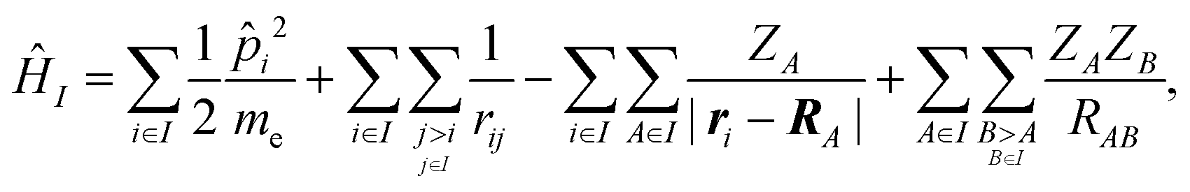 | (1) |
![[p with combining circumflex]](https://www.rsc.org/images/entities/i_char_0070_0302.gif) i is the momentum operator and me is the mass of an electron. ri is the position of electron i, RA is the position of atom A, and ZA is the atomic number of atom A. rij is the distance between electrons i and j, and RAB is the distance between atoms A and B. The ground-state energy EI of the molecule I is
i is the momentum operator and me is the mass of an electron. ri is the position of electron i, RA is the position of atom A, and ZA is the atomic number of atom A. rij is the distance between electrons i and j, and RAB is the distance between atoms A and B. The ground-state energy EI of the molecule I is| EI = 〈ΨI|ĤI|ΨI〉, | (2) |
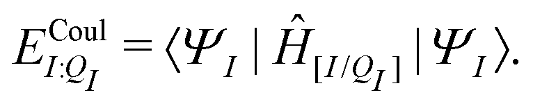
When the molecule I is placed in an embedding field QI = {qF}, the Hamiltonian operator of the embedded molecule is given by ĤI:QI = ĤI + Ĥ[I/QI]. We will use I:QI to denote the embedding of molecule I in the embedding field QI. The Hamiltonian operator Ĥ[I/QI] for Coulomb interactions between the molecule I (QM) and the field QI (MM) is,
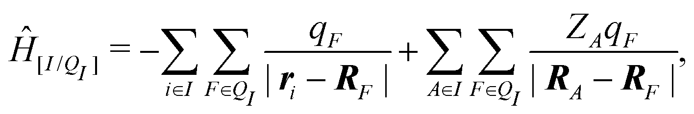 | (3) |
| EI:QI = 〈ΨI:QI|ĤI:QI|ΨI:QI〉, | (4) |
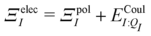
We will use the symbol Ξ to denote a difference between two expectation values. The electronic interaction energy describes the change in electronic energy of a molecule upon interaction with the embedding field,
| ΞelecI = 〈ΨI:QI|ĤI:QI|ΨI:QI〉 − 〈ΨI|ĤI|ΨI〉. | (5) |
| ΞpolI = 〈ΨI:QI|ĤI:QI|ΨI:QI〉 − 〈ΨI|ĤI:QI|ΨI〉, | (6) |
 | (7) |
 . Hensen et al.6 further decomposed the polarization energy ΞpolI into an energy of distorting the gas-phase wave function,
| ΞdistI = 〈ΨI:QI|ĤI|ΨI:QI〉 − 〈ΨI|ĤI|ΨI〉, | (8) |
| ΞstabI = 〈ΨI:QI|Ĥ[I/QI]|ΨI:QI〉 − 〈ΨI|Ĥ[I/QI]|ΨI〉. | (9) |
In a system of N molecules, the total electronic interaction energy and its decomposition into polarization and permanent Coulomb energies are,
| Ξelec = Ξpol + ECoul | (10) |
 | (11) |
 | (12) |
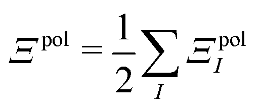
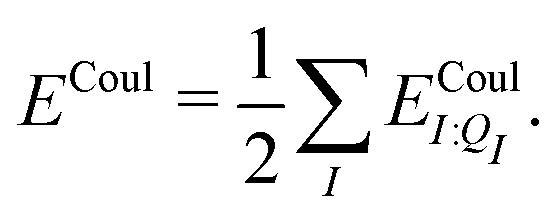
In our present scheme, only one molecule, the ligand, is treated quantum mechanically. Thus Ξelec = ΞelecI, Ξpol = ΞpolI, Ξdist = ΞdistI, Ξstab = ΞstabI, and 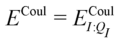 , where I is the ligand molecule.
Both ΨI and ΨI:QI were calculated using the restricted Hartree–Fock method26 in conjunction with the 6-311G** basis set.27 The atomic charge of atoms A with and without the embedding field QI = {qF},  and qQMA, respectively, were obtained by fitting to the quantum mechanical electrostatic potential (ESP) using the restrained electrostatic potential (RESP) method.28 Fitted point charges were used to evaluate the stabilization energy,
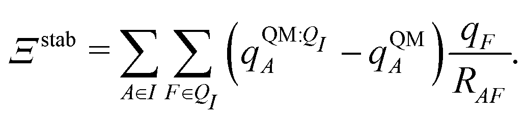 | (13) |
For most reported calculations, the embedding field QI = {qF} consisted of all of the non-ligand atoms in the system. In order to evaluate the distance at which embedding field atoms affect the polarization energy, we also performed calculations in which the embedding field consists of all atoms within a cutoff parameter Rcut of any ligand atom. The cutoff parameter was varied from Rcut ∈ {4,5,…,10,12,…,20}. Even when different Rcut were used for determining ΨI:QI and  , energies were evaluated using an embedding field based on all atoms in the model.
In addition to the electrostatic interaction energy, coupling between the QM and MM region also includes a van der Waals interaction energy modeled by the Lennard-Jones potential,
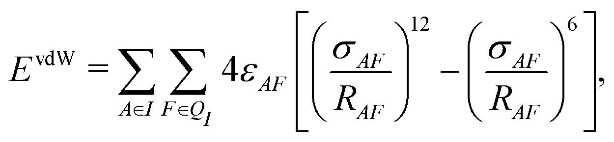 | (14) |
| Epair = ECoul + EvdW. | (15) |
Because we are interested in molecules in solution, opposed to the gas phase, we also consider the solvation free energy. We will use W(X) to denote a solvation free energy, where X ∈ {PL,P,L} represent the complex, protein, and ligand, respectively. The solvation free energy is an integral over all the solvent degrees of freedom. There are many possible ways to compute this quantity. In this paper, we used two continuum dielectric implicit solvent models for the electrostatic component of the solvation free energy: the Onufriev Bashford Case 2 (OBC2)29 generalized Born and domain decomposition COnductor-like Screening MOdel (ddCOSMO).30,31 We will elaborate on how we applied these models in subsequent paragraphs, but here we would like to point out a key distinction between the models: ddCOSMO accounts for polarization of the solute by solvent. On the other hand, the OBC2 model, which was developed for fixed-charge molecular mechanics force fields, does not. The nonpolar cavity formation term in the solvation free energy was calculated as the product of the surface tension γ and surface area A(X).
Given a particular solvation free energy model, the total binding energy is given by (Fig. 1),
| Ψbind = Epair + Ξpol + Wbind, | (16) |
| Wbind = W(PL) − W(P) − W(L). | (17) |
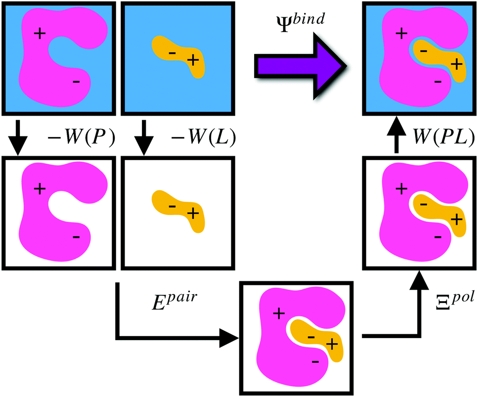 | ||
| Fig. 1 Schematic illustrating the decomposition of binding energy, Ψbind, into desolvation free energy of the protein, −W(P), the desolvation free energy of the ligand, −W(L), the intermolecular pairwise interaction energy, Epair, the ligand polarization energy, Ξpol, and the solvation free energy of the complex, W(PL). | ||
In applying the OBC2 model, which does not explicitly account for polarization by solvent, we used different ligand partial charge schemes. In the WOBC2(PL) calculation,  are used for ligand partial charges. On the other hand, the WOBC2(L) calculation uses qQMA for ligand partial charges. To isolate the effects of polarization by the embedding field, we also define a total binding energy that does not consider ligand polarization,
| Ψbind,npOBC2 = Epair + Wbind,np, | (18) |
| Wbind,npOBC2 = W(PL,np) − W(P) − W(L). | (19) |
In the COnductor-like Screening MOdel (COSMO), the solvent is treated as a set of apparent charges on the surface of the solute cavity. These charges interact with the system according to Coulomb's law, such that,
 | (20) |
For a species X in ddCOSMO solvent, the solvation free energy is given by
| WddCOSMO(X) = ΞelecX,sol + ΔGsurf, | (21) |
The electrostatic components of these energies are given by,
| ΞelecX,sol = 〈ΨX,sol|ĤX,sol|ΨX,sol〉 − 〈ΨX|ĤX|ΨX〉. | (22) |
| ΞpolX,sol = 〈ΨX,sol|ĤY,sol|ΨX,sol〉 − 〈ΨX|ĤY,sol|ΨX〉, | (23) |
| ECoulX,sol = 〈ΨX|Ĥ[Y/sol]|ΨX〉, | (24) |
A helpful way to summarize the effect of polarization by the solvent (in addition to polarization by the embedding field) is
| Ξpolsol = ΞpolPL,sol − ΞpolL,sol. | (25) |
2.2 Other properties
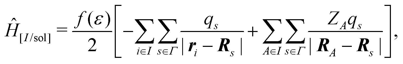
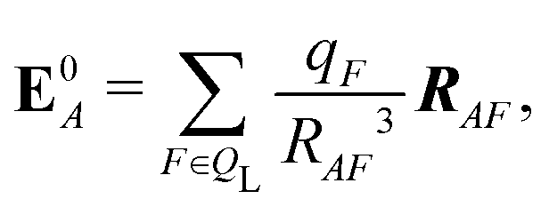
We computed a number of other properties to assess whether they have a clear relationship with the polarization energy.Motivated by the observation of a high density of acid and base side chains in enzymes,1 we computed two quantities: the percentage of atoms in a protein that are highly charged; and the number density of highly charged atoms within 6 Å of any ligand atom. The percentage of atoms in the protein that are highly charged is defined as,
 | (26) |
 | (27) |
We also computed a number of properties inspired by classical electrostatics. In classical electrostatics, the internal energy of a dipole moment in an electric field is the dot product of the dipole with the field. We considered two classical models: one in which the entire ligand is treated as a dipole and a second in which each atom is treated as a dipole.
If the ligand is considered as a dipole, the change in internal energy due to an induced dipole is,
| Ξpol,cL = −μindL·E0L, | (28) |
 | (29) |
The induced dipole moment of the ligand μindL was calculated in two ways. The first was from the expectation value of the dipole moments,
 | (30) |
![[small mu, Greek, circumflex]](https://www.rsc.org/images/entities/i_char_e0b3.gif) is the dipole moment operator. The second was based on the molecular polarizability tensor, αL, and the electric field on the center of mass of the ligand,
is the dipole moment operator. The second was based on the molecular polarizability tensor, αL, and the electric field on the center of mass of the ligand, | (31) |
 | (32) |
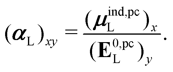
 , could potentially reduce the computational costs of Ξpol prediction. To facilitate comparison with the polarization energy, we also computed the molecular polarizability scalar of the ligand, αL, defined as,
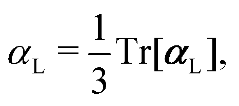 | (33) |
If each atom on the ligand is considered as a dipole, then the change in internal energy due to an induced dipole is,
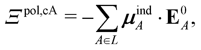 | (34) |
 | (35) |
 | (36) |
In all, we considered the relationship between Ξpol and a number of other properties: the
(1) percentage of highly charged atoms in a protein (eqn (26));
(2) molecular polarizability scalar, αL (eqn (33));
(3) Coulomb interaction energy, ECoul (eqn (7));
(4) magnitude of the electric field on the ligand center of mass, |E0L|, where E0L is from eqn (29);
(5) magnitude of total electric field on the ligand atom sites,  , where E0A is from eqn (35);
(6) magnitude of the induced dipole moment based on wave functions, |μind,QML|, where μind,QML is from eqn (30);
(7) magnitude of the induced dipole moment based on the molecular polarizability tensor,  , where
  is from eqn (31);
(8) classical polarization energy of a ligand dipole, Ξpol,cL (eqn (28)), using eqn (30) for the induced dipole moment;
(9) classical polarization energy of a ligand dipole, Ξpol,cL,αL (eqn (28)), using eqn (31) for the induced dipole moment;
(10) classical polarization energy of atomic dipoles, Ξpol,cA (eqn (34));
(11) and ligand polarization energy including solvent effects, Ξpolsol (eqn (25)).
2.3 Computational methods
Structures from the PDBBind Core Set (release 2016) were processed through an automated workflow based on AmberTools 1738 and customized QM/MM codes. Protein protonation states were assigned using PDB2PQR 1.9.0 at a pH of 7.0 and ligand protonation states using pkatyper in the QUACPAC 1.7.0.2 toolkit (OpenEye). AMBER topology files based on protein and cation parameters (Na+, Mg2+, Ca2+, and Zn2+) from the AMBER ff14SB force field39 and ligand parameters from the Generalized AMBER Force Field 240 were built using AmberTools 17.38Using OpenMM 7.3.1,41 complexes in OBC229 generalized Born/surface area implicit solvent were minimized with heavy atom restraints of 2 kcal mol−1 Å−2 towards crystallographic positions until energies converged within 0.24 kcal mol−1.
In our modified QM/MM codes, the evaluation of molecular integrals of many-body operators over Gaussian functions were obtained using libint 2.5.042 and the linear algebra and eigenvalue decomposition of a symmetric matrix were done with the Armadillo 8.500.1.43,44
OpenMM 7.3.141 was also used to evaluate van der Waals and solvation energies, the latter with the OBC229 generalized Born/surface area implicit solvent model. It was also used for the ΔGsurf term in eqn (21). The PySCF 1.7.0 python package45 was used to perform QM/MM calculations in the ddCOSMO scheme.30,31
3 Results and discussion
3.1 The distribution of polarization energy is broad and skewed
Signs of the calculated polarization energy Ξpol, the distortion energy Ξdist, and the stabilization energy Ξstab are mostly as expected (Fig. 2). In nearly all of the calculations, Ξpol < 0, Ξdist > 0, and Ξstab < 0. The embedding field reshapes the wave function to have stronger Coulomb interactions between the electronic probability density and point charges, such that Ξstab < 0. Because the gas-phase wave function of the ligand has the optimal intramolecular potential, perturbing the wave function leads to a higher intramolecular potential energy such that Ξdist > 0. In the vast majority of systems, the calculated distortion is more than compensated for by the calculated stabilization such that the calculated net effect on the interaction energy due to polarization, Ξpol, is negative.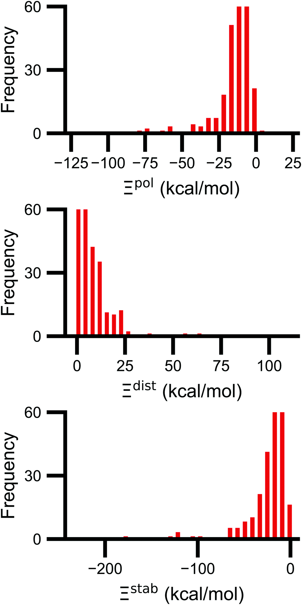 | ||
| Fig. 2 Histograms of the ligand polarization (top, Ξpol), distortion (middle, Ξdist), and stabilization (bottom, Ξstab) energies in the PDBBind Core Set. The three quantities are related by Ξpol = Ξdist + Ξstab. | ||
Exceptions to the trend of negative calculated ligand polarization energies are due to structural modeling issues that lead to short intermolecular distances. Positive Ξpol values were calculated in three complexes. In our models of these structures, there are very short distances between a hydrogen atom in the ligand and in the protein: 0.73 Å in 2fxs, 1.06 Å in 3u5j, and 0.87 Å in 4f2w. The close proximity of atoms leads to a severe distortion in the wave function that is not overcome by more favorable Coulomb interactions. These steric clashes could be resolved by changing the models in minor ways that are equally compatible with crystallographic evidence and pKa predictions. In the 2fxs and 4f2w models, the proton on a carboxylic acid was arbitrarily placed near a ligand hydrogen instead of on the other carbonyl oxygen. In the 3u5j model, the clash could be resolved by switching the position of the terminal oxygen and amine groups, which have nearly identical electron density, on asparagine 140.
The distribution of Ξpol, Ξdist, and Ξstab is broad and skewed. There is a peak in the distribution of Ξpol around −10 kcal mol−1. However, for a small number of complexes, Ξpol is much lower, with a minimum value of −128 kcal mol−1.
3.2 Systems with the lowest Ξpol have close cations
We hypothesized that the lowest Ξpol could be due to crystallographic cations. To test this hypothesis, we subdivided the PDBBind Core Set into two subsets: 90 complexes with cations (Na+, Mg2+, Ca2+, and Zn2+) and 196 complexes without cations in the crystal structure.Histograms of Ξpol for the two subsets are consistent with our hypothesis (Fig. S1 in the ESI†). All systems in which Ξpol < −50 kcal mol−1 are in the subset with cations. In contrast, the minimum Ξpol in the subset without cations is around −40 kcal mol−1. The range of Ξdist and Ξstab is also much smaller in the subset without cations.
Crystallographic cations may have an outsize role in ligand polarization because the magnitude of their charge is larger than the charge of most protein atoms. In the AMBER ff14SB force field,39 protein partial charges were determined by applying RESP28 to electrostatic potentials from QM calculations. Most protein atoms have near-zero charge. The magnitude of the charge is greater than 0.6e, where e represents the elementary charge, in only a few atoms. It is less than 1e in all atoms. These conclusions are also true for protein atoms in our data set (Fig. S2 in the ESI†). The low magnitude of charge results from delocalization of net charges across several atoms. In contrast, the cations have a charge of +1e or +2e that is localized onto a single atom and have a more focused effect on the electrostatic potential.
Beyond the presence of cations, the distance between ligand and cation atoms also plays an important role in ligand polarization (Fig. 3). Even if cations are present in a crystal structure, they are not necessarily close enough to the ligand to significantly polarize its wave function. In many systems, cations are over 10 Å from any ligand atom. In all of the complexes in which Ξpol < −50 kcal mol−1, a cation is within 4 Å of a ligand atom.
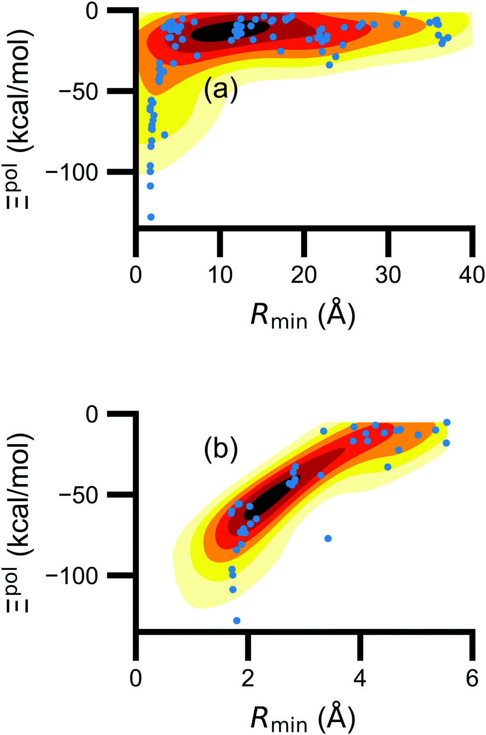 | ||
| Fig. 3 Scatter plot of the ligand polarization energy Ξpol as a function of the minimum distance between a ligand and cation atom, Rmin, for (a) the entire range of Rmin and (b) Rmin < 6 Å. | ||
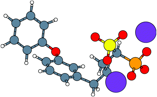
Unfortunately, the extent of ligand polarization when ligands are close to cations is likely overestimated by our QM/MM scheme. Because only the ligand is included in the QM region, cations are simply represented as positive point charges. While actual cations have inner-shell electrons that repel further electron density, the point charges are purely attractive. The purely attractive forces draw an unrealistic amount of electron density between the ligand and cation, leading to a very negative polarization energy. For an estimate of the extent of overpolarization in several systems, see Table S1 in the ESI.† As an illustrative example, there is a significant gain in the electron density between the ligand and cation in the complex 3dx1 (Fig. 4). Hence, we will proceed with extra caution in interpreting points where Ξpol < −50 kcal mol−1.
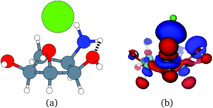 | ||
| Fig. 4 (a) The molecular structure of the ligand with one zinc cation Zn2+ in the complex 3dx1. Hydrogen, carbon, nitrogen, oxygen, and zinc atoms are colored with white, gray, blue, red, and green, respectively. (b) The difference in the electronic probability density is plotted. Blue and red contours illustrate the gain and loss of the electronic probability density due to the embedding field. | ||
3.3 The importance of the embedding field size diminishes with distance
The size of the embedding field strongly affects estimates of the polarization energy (Fig. 5). Changes in the cutoff distance Rcut alter the partial charges included in the embedding field, the wave function ΨI:QI, and then the RESP charges. Regardless of Rcut, nearly every estimate of ΔΞpol(Rcut) = Ξpol(Rcut) − Ξpol(Rcut = ∞) is positive, indicating that the ligand wave function accommodates even distant charges in the embedding field. However, the influence of protein and cation charges diminishes with distance. Correspondingly, as ΔΞpol diminishes, so does its variance. For larger values of Rcut = 8, 9, 10, and 12 Å, the mean (and standard deviation) of ΔΞpol is 1.81 (1.77), 1.49 (1.80), 1.10 (1.23), and 0.92 (1.14) kcal mol−1, respectively. | ||
| Fig. 5 Dependence of the Coulomb interaction ECoul, the ligand polarization energy Ξpol, and the distortion energy Ξdist on the cutoff distance Rcut. Here, the deviation and the gradient are defined as ΔF(Rcut) = F(Rcut) − F(∞) and G = dF(Rcut)/dRcut, respectively, where F is either E or Ξ. In these violin plots, the width of the shaded area is proportional to the frequency of observations. Large blue points are placed at mean values. In the plot of ΔΞpol as a function of Rcut, the green line is a function that was fitted to the mean values, 80.778Rcut−2 + 0.177. | ||
The decomposition of the polarization energy into ECoul and Edist is more sensitive to Rcut than the polarization energy itself; distributions of the values (relative to values with no cutoff) and numerical derivatives are broader. Even at Rcut = 8, 9, 10, and 12 Å, the mean (and standard deviations) of ΔECoul are −2.28 (4.94), −1.46 (4.71), −1.18 (4.06), and −0.99 (3.38) kcal mol−1.
On average, the decay of ΔΞpol is well-described by an inverse square law. A nonlinear least-squares regression using scipy.optimize.curve_fit (https://scipy.org/) of x1Rcut−2 + x2 for x1 and x2 yielded a curve that closely matches the data. The curve is best for low Rcut, slightly underestimates the mean for intermediate Rcut, and slightly overestimates the mean for larger Rcut. The inverse square power law is consistent with the R−4 dependence of ion-induced dipole interactions because the volume of the region containing embedding field charges increases as Rcut2.
3.4 Of computed properties, Ξpol is most correlated with the electric field, the induced dipole moment, and the classical polarization energy
We observed that a number of properties – the percentage of atoms in a protein that are highly charged, the number density of highly charged atoms, and the Coulomb interaction energy – have little or only weak correlation with the ligand polarization energy (Fig. S3 in the ESI†). We also observed that the molecular polarizability scalar (αL) has a strong linear correlation with the number of electrons in the system (Fig. S4 in the ESI†) but not with the ligand polarization energy.In contrast with the aforementioned properties, there is a much clearer relationship between the ligand polarization energy, Ξpol, and several other properties: the magnitude of the electric field; the magnitude of the induced dipole moment of the ligand; and the classical polarization energy (Fig. 6). The linear correlation is strong with the magnitude of the electric field on the ligand center of mass, |E0L|, and even stronger with the magnitude of the total electric field vector active on all ligand atoms,  (Fig. 6 and Fig. S5 in the ESI†). Intriguingly, in both cases, there appear to be two distinct trends relating the electric field to the magnitude of the electric field; a linear correlation exists in systems where Ξpol < −50 kcal mol−1, but the slope is distinct from in systems where −50 kcal mol−1 < Ξpol < 0 kcal mol−1. The two measures of the electric field are also correlated with each other, with a Pearson's R of 0.54 (Fig. S6 in the ESI†). Similarly, the ligand polarization energy Ξpol is also strongly correlated with the magnitude of the induced dipole moment of the ligand. There is a stronger correlation with the magnitude of the induced dipole moment based on wave functions |μind,QML|, where μind,QML is from eqn (30), than the magnitude of the induced dipole moment based on the molecular polarizability tensor,
  , where
  is from eqn (31) (Fig. 6 and Fig. S7 in the ESI†).
 | ||
| Fig. 6 The ligand polarization energy, Ξpol, as a function of the magnitude of the electric field |E0L| (top), the magnitude of the induced dipole moment |μind,QML| (middle), and the classical polarization energy Ξpol,cL (bottom), where E0L, μind,QML, and Ξpol,cL are from eqn (29), (30), and (28), respectively. The range of Ξpol is either Ξpol < 0 kcal mol−1 (left) or −50 kcal mol−1 < Ξpol < 0 kcal mol−1 (right). | ||
Finally, in addition to the strong relationship between the ligand polarization energy Ξpol and both the magnitude of the electric field and the induced dipole, there is also a clear correspondence between the ligand polarization energy Ξpol and the classical polarization energy. Of approaches to compute the classical polarization energy, treating the entire ligand as a dipole and using eqn (30) for the induced dipole moment led to the best correlation with the quantum polarization energy (Fig. 6 and Fig. S8 in the ESI†). The clear correlation between the two quantities suggests that the classical model of a dipole in an electric field is a reasonable explanation for the quantum behavior. Limitations of the molecular polarizability model are described in Fig. S9 and S10 in the ESI.†
The observed linear correlation between the ligand polarization energy and the magnitude of the electric field |E0L| (Fig. 6) has potential implications for modeling protein–ligand interactions with MM, including molecular docking. Because |E0L| is computed without a QM calculation, a relatively inexpensive polarization energy estimate based on linear regression can be added to binding energy estimates. Such an approach could recapitulate some of the success of semi-empirical QM in reconstructing binding poses.12–15
3.5 Polarization is a substantial and variable fraction of interaction and binding energies
We observe that the ligand polarization energy Ξpol can be a substantial and highly system-dependent fraction of the interaction energy and binding energy (Fig. 7). In most systems where −50 kcal mol−1 < Ξpol < 0 kcal mol−1, the ratio Ξpol/Ξelec ranges from 0 to 0.4 (Fig. 7a). Exceptions occur when Ξelec is positive, leading to a negative ratio, or when it is small, leading to a ratio much larger than 1 (Table S2 in the ESI†). Positive and small values of Ξelec result from positive ECoul. For example, the complex 5c2h has Ξpol = −22.45 kcal mol−1, ECoul = 19.60 kcal mol−1, and Ξelec = −2.85 kcal mol−1. Hence, Ξpol/Ξelec = −7.88. The histogram of Ξpol/(Epair + Ξpol) is compressed compared to Ξpol/Ξelec, with the range with the largest density reduced to between 0 and 0.2 (Fig. 7b). Smaller ratios are due to the addition of van der Waals interactions that increase values in the denominator. The histograms of Ξpol/(Ψbind,npOBC2 + Ξpol) and Ξpol/ΨbindOBC2 is notable for a clear peak around 0.2 (Fig. 7c and d). If all systems in the PDBBind are considered, qualitative trends are similar but there is increased density at higher ratios (Fig. S11 in the ESI†).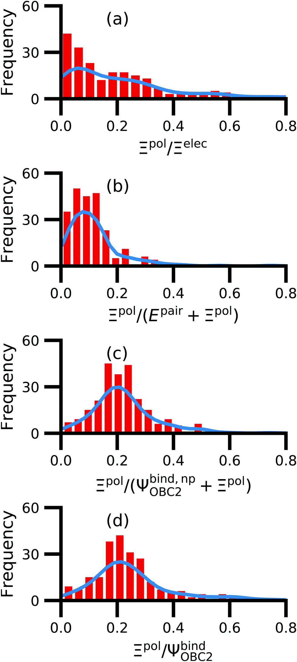 | ||
| Fig. 7 Histograms of ratio of the polarization energy of the ligand to (a) the electrostatic interaction (Ξelec = ECoul + Ξpol), (b) the intermolecular pairwise potential energy with the ligand polarization energy (Epair + Ξpol), (c) the binding energy without considering ligand polarization in the solvation free energy (Ψbind,npOBC2 + Ξpol), and (d) the binding energy with considering ligand polarization in the solvation free energy (ΨbindOBC2). The histograms are truncated at a ratio of 1.25. Data are only included for complexes where Ξpol < 0 kcal mol−1 (left) or −50 kcal mol−1 < Ξpol < 0 kcal mol−1. For analogous histograms including all data, see Fig. S11 in the ESI.† | ||
When considering the polarization energies of three HIV-protease inhibitors, Hensen et al.6 found that Ξpol can approach one-third of the electrostatic interaction energy. In our much larger data set, we found that Ξpol can be a larger fraction of Ξelec.
With the caveat that polarization could be overestimated in these cases, two examples where Ξpol/(Ψbind,npOBC2 + Ξpol) is particularly large, 3dx1 and 3dx2, highlight the potentially outsized importance of Ξpol for small ligands (Table S2 in the ESI†). In 3dx1, Ψbind,npOBC2 + Ξpol = −12.953 kcal mol−1, Ξpol = −80.77 kcal mol−1, and the ratio is Ξpol/(Ψbind,npOBC2 + Ξpol) = 6.236. For comparison, in 2zcq, Ψbind,npOBC2 + Ξpol = −295.48 kcal mol−1, Ξpol = −128.01 kcal mol−1, and the ratio is Ξpol/(Ψbind,npOBC2 + Ξpol) = 0.43. The ligand in 3dx1 (Fig. 4) is much smaller than the ligand in 2zcq (Fig. 8). Small ligands have fewer opportunities for pairwise contacts with their protein binding partners than larger ligands. The limited number of contacts leads to a weaker Ψbind,npOBC2, such that Ξpol can play a larger role.
 | ||
| Fig. 8 The molecular structure of the ligand with two magnesium cations Mg2+ in the complex, 2zcq. Hydrogen, carbon, oxygen, magnesium, phosphorus, and sulfur atoms are colored with white, gray, red, pink, orange, and yellow, respectively. | ||
The relative importance of ligand polarization in small ligands may explain the poor performance of binding free energy methods based on a fixed-charge force field in distinguishing molecules that are active and inactive against T4 lysozyme L99A.46 In this protein, the L99A mutation forms a pocket known to bind a number of small hydrophobic compounds. Xie et al.46 performed binding free energy calculations for a library of 141 small hydrophobic compounds whose thermal activity against T4 lysozyme L99A had been measured. Many of the compounds contained highly polarizable aromatic groups. The best-performing method in Xie et al.46 had an area under the receiver operating characteristic curve of 0.74 (0.04) out of 1 for a perfect binary classifier. Binary classification performance could potentially be improved by incorporating the ligand polarization, as described in the current paper.
3.6 Solvent usually has a small effect on ligand polarization
In the vast majority of systems, polarization of the ligand is similar whether solvent is considered or not (Fig. 9). The difference between Ξpolsol and Ξpol has a mean of 2.0 kcal mol−1 and standard deviation of 6 kcal mol−1. Only a small percentage (7%) of the scatter plot for the two quantities deviate from linearity (y = x) by more than 10 kcal mol−1, such that |Ξpolsol − Ξpol| > 10 kcal mol−1 (Fig. S12 in the ESI†). While the scatter plot focuses on the range where −40 kcal mol−1 < Ξpolsol < 0 kcal mol−1, the same trend, in which the embedding field dominates ligand polarization energies, holds true for even lower Ξpolsol. In most complexes, ligands are embedded in their respective receptors. When the ASCs are far from the ligand, they have a minimal effect on the electric field experienced by the ligand and on the ligand polarization energy.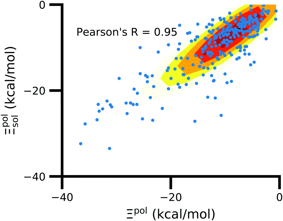 | ||
| Fig. 9 Solvent effect on the ligand polarization energies of the ligand–protein complexes. The axes are limited to a range of −40 kcal mol−1 < Ξpol < 0 kcal mol−1. | ||
There are small number of systems in which the ligand is polarized by the solvent much more so than by the protein. These are exceptions rather than the rule. They can only occur when the ligand is exposed to the surface and the protein generates a strong electrostatic potential at the surface.
Further underscoring the relatively limited effect of solvent on ligand polarization energies, solvation free energies calculated with and without polarization by solvent are highly correlated (Fig. 10). If solvent had a large effect on ligand polarization, the solvation free energy estimate from the OBC2 model, which does not treat solvent-induced ligand polarization, would have a markedly different trend than ddCOSMO model, which does. Instead, the Pearson R between the two estimates is nearly 1.
 | ||
| Fig. 10 Comparison of solvation free energy estimates (in kcal mol−1) based on OBC2 (x-axis) and ddCOSMO (y-axis). Solvation free energy estimates are of the (a) ligand, (b) protein, (c) complex, and (d) the binding energy. | ||
Although the solvation free energy estimates are very correlated, there is small systematic difference between the implicit solvent models. For the ligand, protein, complex, and binding energy, the slope (and intercept) are 0.94 (5.7), 1.04 (121.6), 1.04 (99.2), and 0.96 (−18.1). The shift in the intercept suggests a systematic error in one of the models.
3.7 Solvation and polarization can be key drivers of native complex formation
For a number of native complexes, both polarization and solvation were required to compute negative binding energies (Fig. 11). Due to the harmonic restraint maintained during minimization, our models closely resemble their native crystal structures. In order for these protein–ligand complexes to adopt these structures, they should have a negative binding energy (presuming that binding results in entropy loss). Intriguingly, the Coulomb interaction energy is positive in a significant fraction of these systems (Fig. 11a). Incorporating van der Waals interactions in Epair slightly reduces the number of systems in which the interaction energy is positive (Fig. 11c). However, these pairwise terms, which are standard to molecular docking, are insufficient to accurately describe all the native complexes with a negative interaction energy. Incorporating a ligand polarization term (Fig. 11b and d) or nonpolarizable solvation energy term (Fig. 11e and g) alone is also insufficient. However, when both polarization and solvation are considered, all the native complexes have a negative binding energy (Fig. 11f, h, i and j) (Fig. 11i removes ligand polarization but the solvation energy still considers polarization.) Considering both polarization and solvation terms also appears to attenuate the broad range of binding energies observed in Epair, Epair + Ξpol, and Ψbind,np (Fig. 11f, h, i and j). Using the partial charges qQMA opposed to does not have a qualitative effect on these trends. The trends also hold for systems within the normal range of −50 < Ξpol < 0 kcal mol−1 (Fig. S13 in the ESI†). The importance of including ligand polarization and solvation was previously noted by Kim and Cho,17 who achieved superior performance at binding pose prediction using a protocol that combined atomic charges from QM/MM with solvation compared to using either by themselves.
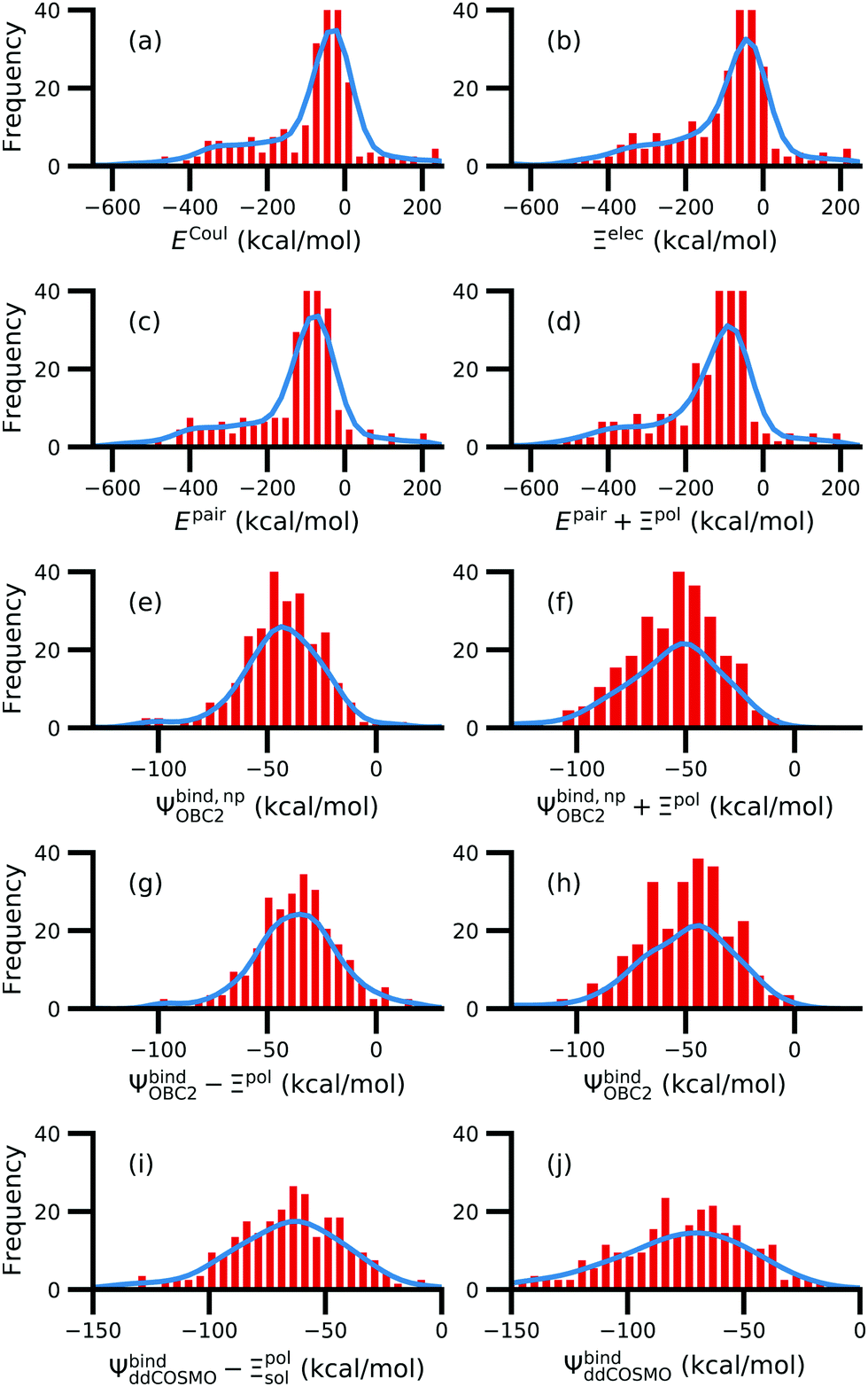 | ||
| Fig. 11 Histograms of intermolecular potential energies and binding energies. The intermolecular potential energies are (a) the permanent Coulomb interaction (ECoul), (b) the electrostatic interaction (Ξelec = ECoul + Ξpol), (c) the intermolecular pairwise potential energy (Epair = EvdW + ECoul), and (d) the intermolecular pairwise potential energy with the polarization energy of the ligand (Epair + Ξpol) in the gas phase. The OBC2 binding energies are (e) without considering ligand polarization at all, Ψbind,npOBC2, (f) considering ligand polarization for electrostatic interactions but not in the solvation free energy, Ψbind,npOBC2 + Ξpol, (g) considering ligand polarization in the solvation free energy but not for electrostatic interactions, ΨbindOBC2 − Ξpol, (h) considering ligand polarization both in the electrostatic interactions and the solvation free energy. The ddCOSMO binding energies are (i) without and (j) with the ligand polarization energy. A similar plot that only considers systems for which −50 < Ξpol < 0 kcal mol−1 is available as Fig. S13 in the ESI.† | ||
The lowest ECoul are due to phosphate groups. The lowest ECoul is observed in the complex 2zcq. The complex contains two Mg2+ in close proximity to a negatively-charged phosphate group (Fig. 8). The complex 1u1b also has a very low ECoul. The ligand in 1u1b contains four phosphates (Fig. S14 in the ESI†). RESP charges on the phosphorus are around 1.4e and oxygen charges range from −0.4 to 0.8e, leading to a low ECoul.
3.8 Solvation but not polarization improves correlation with experimental binding free energies
An important goal in protein–ligand modeling is the accurate calculation of binding free energies – which quantify the strength of noncovalent association – that are consistent with experimentally observed values.For several reasons, the computed binding energy ΔGbind is not expected to completely agree with the experimentally measured binding free energy ΔGbind for complexes in the PDBBind Core Set. These reasons include that:
• The binding free energy ΔGbind is not rigorously equivalent to Ψbind, but is actually an exponential average over the ensemble of the complex.47,48 Using Ψbind to model ΔGbind is an approximation that neglects entropy.
• The binding energy model is not exact. For example, the present model does not explicitly treat polarization of the free ligand by solvent, polarization of the protein by the ligand, and the solvation model does not include explicit water.
• The PDBBind is a heterogeneous data set in which experimental ΔGbind were determined by various modalities and under different experimental conditions. There may be systematic differences between measured ΔGbind that are not considered in our models.
• On a related note, experimental conditions used to obtain crystal structures and binding affinity data are different. Crystal structures have packing forces and are generally at a lower temperature.
Nonetheless, a comparison between computed interaction energies and experimental binding free energies can be informative.
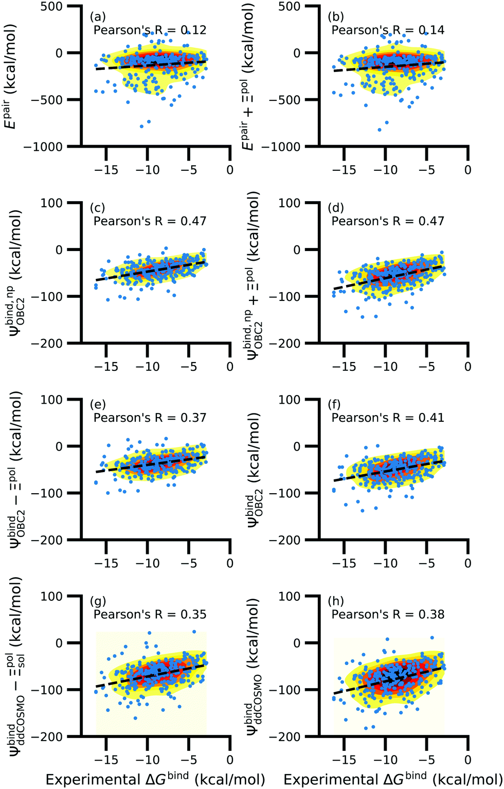
While the treatment of solvation is essential, ligand polarization energies have a minimal effect on the correlation between Ψbind and experimental ΔGbind (Fig. 12 and Fig. S15 in the ESI†). If solvation energies are not considered, the distribution of intermolecular pairwise potential energies Epair of the protein–ligand complexes is distributed extremely broadly from −1000 kcal mol−1 to 250 kcal mol−1 and the correlation between Ψbind and experimental ΔGbind is negligible (Fig. 12a, b and Fig. S15a, b in the ESI†). Incorporating solvation but not polarization significantly improves Pearson's R to 0.47 for complexes where −50 kcal mol−1 < Ξpol < 0 kcal mol−1 and 0.44 for complexes where Ξpol < 0 kcal mol−1 (Fig. 12c and Fig. S15c in the ESI†). Although the range of computed binding energies is dramatically reduced to −200 kcal mol−1 to 0 kcal mol−1, it is still very broadly distributed compared to the distribution of experimentally measured binding free energies (−16 kcal mol−1 < ΔGbind < −3 kcal mol−1), supporting the idea that a single structure cannot represent an ensemble of structures obtained in experimental conditions. Adding the polarization energy to solvation energies computed without solvation has no effect on the solvation energy (Fig. 12d and Fig. S15d in the ESI†). In comparison, computing solvation energies using partial charges from the induced dipole diminishes correlation with experiment (Fig. 12e, f and Fig. S15e, f in the ESI†). The solvation energy computed with ddCOSMO demonstrates similar performance (Fig. 12g, h and Fig. S15g, h in the ESI†).
 | ||
| Fig. 12 Comparison of interaction energies (in kcal mol−1) to experimentally measured binding free energies (in kcal mol−1) for complexes with −50 kcal mol−1 < Ξpol < 0 kcal mol−1. Interaction energies are according to (a) the intermolecular pairwise potential energy (Epair = EvdW + ECoul) and (b) the intermolecular pairwise potential energy with the polarization energy of the ligand (Epair + Ξpol) in the gas phase. Panels (c–h) are binding energies, with (c–f) based on the OBC2 and (g and h) based on the ddCOSMO implicit solvent models. The OBC2-based binding energies are: (c) Without considering ligand polarization at all, Ψbind,npOBC2; (d) considering ligand polarization for electrostatic interactions but not in the solvation free energy, Ψbind,np + Ξpol; (e) considering ligand polarization in the solvation free energy but not for electrostatic interactions, Ψbind − Ξpol; or (f) considering ligand polarization both in the electrostatic interactions and the solvation free energy. The ddCOSMO-based binding energies are (g) without and (h) with considering the ligand polarization energy. A similar plot for all complexes is available as Fig. S15 in the ESI.† | ||
In a critical assessment of a number of docking programs and scoring functions across eight different diverse proteins, Warren et al.49 concluded that “no statistically significant relationship existed between docking scores and ligand affinity.” Our data suggest that the lack of correlation stems from a poor or nonexistent treatment of solvation in the scoring functions. Perhaps due to cancellation of error, neglect of ligand polarization does not appear to be a major factor in the poor performance of docking scores.
4 Conclusions
Using QM/MM6,23,50,51 with and without ddCOSMO implicit solvent,30,31 we computed polarization energies (Ξpol and Ξpolsol) for 286 complexes in the PDBBind Core Set.25 The distributions of Ξpol, Ξdist, and Ξstab were found to be broad and skewed. For properly prepared systems without atoms in unrealistically close contact, these terms all have the expected sign of Ξpol < 0, Ξdist > 0, and Ξstab < 0. The lowest Ξpol were observed in systems where cations are close to ligand atoms. In these systems, the extent of polarization is likely to be overestimated. The importance of including embedding field charges on Ξpol appears to diminish, on average, as an inverse square law. There is no clear relationship between Ξpol and the percentage of highly charged atoms in a protein and molecular polarizability scalar. There is a weak correlation between Ξpol and the Coulomb energy ECoul. On the other hand, there is a stronger linear correlation between Ξpol and the magnitude of the electric field, the magnitude of the induced dipole moment, and the classical polarization energy. The ligand polarization energy Ξpol is observed to a substantial and system-dependent fraction of the electronic interaction energy and the total interaction energy. In most cases, the effect of the implicit solvent on the ligand polarization energy is minor. In some systems, consideration of ligand polarization and solvation are both essential for calculating negative interaction energies for crystallographic complexes. While consideration of solvation is essential for achieving moderate correlation between interaction energies and experiment, we did not observe that the ligand polarization energy Ξpol improves the correlation between the binding energy and experimental binding free energies.Conflicts of interest
There are no conflicts to declare.Acknowledgements
We thank Pengyu Ren for the suggestion to compare polarization energies with molecular polarizability. We thank Filippo Lipparini and Qiming Sun for valuable discussions and implementation of QM/MM/ddCOSMO. We thank OpenEye Scientific Software, Inc. for providing academic licenses to their software. This research was supported by the National Institutes of Health (R01GM127712).Notes and references
- D. Jimenez-Morales, J. Liang and B. Eisenberg, Eur. Biophys. J., 2012, 41, 449–460 CrossRef CAS PubMed.
- W. M. Haynes, CRC Handbook of Chemistry and Physics, CRC Press, 94th edn, 2016 Search PubMed.
- B. Honig and A. Nicholls, Science, 1995, 268, 1144–1149 CrossRef CAS PubMed.
- M. Garcia-Viloca, D. G. Truhlar and J. Gao, J. Mol. Biol., 2003, 327, 549–560 CrossRef CAS PubMed.
- M. W. van der Kamp, F. Perruccio and A. J. Mulholland, Proteins: Struct., Funct., Bioinf., 2007, 69, 521–535 CrossRef CAS PubMed.
- C. Hensen, J. C. Hermann, K. Nam, S. Ma, J. Gao and H.-D. Höltje, J. Med. Chem., 2004, 47, 6673–6680 CrossRef CAS PubMed.
- Y. Shi, Z. Xia, J. Zhang, R. Best, C. Wu, J. W. Ponder and P. Ren, J. Chem. Theory Comput., 2013, 9, 4046–4063 CrossRef CAS PubMed.
- Z. Jing, C. Liu, S. Y. Cheng, R. Qi, B. D. Walker, J.-P. Piquemal and P. Ren, Annu. Rev. Biophys., 2019, 48, 371–394 CrossRef CAS PubMed.
- D. Jiao, P. A. Golubkov, T. A. Darden and P. Ren, Proc. Natl. Acad. Sci. U. S. A., 2008, 105, 6290–6295 CrossRef CAS PubMed.
- U. Ryde and P. Söderhjelm, Chem. Rev., 2016, 116, 5520–5566 CrossRef CAS PubMed.
- A. Crespo, A. Rodriguez-Granillo and V. T. Lim, Curr. Top. Med. Chem., 2017, 17, 2663–2680 CrossRef CAS PubMed.
- P. Chaskar, V. Zoete and U. F. Röhrig, J. Chem. Inf. Model., 2014, 54, 3137–3152 CrossRef CAS PubMed.
- A. Pecina, R. Meier, J. Fanfrlík, M. Lepšík, J. Řezáč, P. Hobza and C. Baldauf, Chem. Commun., 2016, 52, 3312–3315 RSC.
- A. Pecina, S. Haldar, J. Fanfrlík, R. Meier, J. Řezáč, M. Lepšík and P. Hobza, J. Chem. Inf. Model., 2017, 57, 127–132 CrossRef CAS PubMed.
- H. Ajani, A. Pecina, S. M. Eyrilmez, J. Fanfrlík, S. Haldar, J. Řezáč, P. Hobza and M. Lepšík, ACS Omega, 2017, 2, 4022–4029 CrossRef CAS PubMed.
- A. E. Cho, V. Guallar, B. J. Berne and R. Friesner, J. Comput. Chem., 2005, 26, 915–931 CrossRef CAS PubMed.
- M. Kim and A. E. Cho, Phys. Chem. Chem. Phys., 2016, 18, 28281–28289 RSC.
- S. Y. Willow, X. C. Zeng, S. S. Xantheas, K. S. Kim and S. Hirata, J. Phys. Chem. Lett., 2016, 7, 680–684 CrossRef CAS PubMed.
- S. Yoo, Y. A. Lei and X. C. Zeng, J. Chem. Phys., 2003, 119, 6083–6091 CrossRef CAS.
- T.-M. Chang and L. X. Dang, Chem. Rev., 2006, 106, 1305–1322 CrossRef CAS PubMed.
- C. Caleman, J. S. Hub, P. J. van Maaren and D. van der Spoel, Proc. Natl. Acad. Sci. U. S. A., 2011, 108, 6838–6842 CrossRef CAS.
- P. Bajaj, A. W. Götz and F. Paesani, J. Chem. Theory Comput., 2016, 12, 2698–2705 CrossRef CAS PubMed.
- J. Gao and X. Xia, Science, 1992, 258, 631–635 CrossRef CAS PubMed.
- P. Fong, J. P. McNamara, I. H. Hillier and R. A. Bryce, J. Chem. Inf. Model., 2009, 49, 913–924 CrossRef CAS PubMed.
- Z. Liu, M. Su, L. Han, J. Liu, Q. Yang, Y. Li and R. Wang, Acc. Chem. Res., 2017, 50, 302–309 CrossRef CAS PubMed.
- A. Szabo and N. S. Ostlund, Modern Quantum Chemistry, Dover Publications, 1996 Search PubMed.
- R. Krishnan, J. Binkley, R. Seeger and J. Pople, J. Chem. Phys., 1980, 72, 650–654 CrossRef CAS.
- C. I. Bayly, P. Cieplak, W. Cornell and P. A. Kollman, J. Phys. Chem., 1993, 97, 10269–10280 CrossRef CAS.
- A. Onufriev, D. Bashford and D. A. Case, Proteins: Struct., Funct., Bioinf., 2004, 55, 383–394 CrossRef CAS PubMed.
- F. Lipparini, B. Stamm, E. Cancés, Y. Maday and B. Mennucci, J. Chem. Theory Comput., 2013, 9, 3637–3648 CrossRef CAS PubMed.
- F. Lipparini, G. Scalmani, L. Lagardére, B. Stamm, E. Cancés, Y. Maday, J.-P. Piquemal, M. J. Frish and B. Mennucci, J. Chem. Phys., 2014, 141, 184108 CrossRef PubMed.
- M. L. Connolly, Science, 1983, 221, 709–713 CrossRef CAS PubMed.
- T. J. Richmond, J. Mol. Biol., 1984, 178, 63–89 CrossRef CAS PubMed.
- A. Bondi, J. Phys. Chem., 1964, 68, 441–451 CrossRef CAS.
- A. Klamt, Wiley Interdiscip. Rev.: Comput. Mol. Sci., 2018, 8, e1338 Search PubMed.
- M. Schaefer, C. Bartels, F. Leclerc and M. Karplus, J. Comput. Chem., 2001, 22, 1857–1879 CrossRef CAS PubMed.
- S. Y. Willow, M. A. Salim, K. S. Kim and S. Hirata, Sci. Rep., 2015, 5, 14358 CrossRef CAS PubMed.
- D. Case, D. Cerutti, I. T. E. Cheatham, T. Darden, R. Duke, T. Giese, H. Gohlke, A. Goetz, D. Greene, N. Homeyer, S. Izadi, A. Kovalenko, T. Lee, S. LeGrand, P. Li, C. Lin, J. Liu, T. Luchko, R. Luo, D. Mermelstein, K. Merz, G. Monard, H. Nguyen, I. Omelyan, A. Onufriev, F. Pan, R. Qi, D. Roe, A. Roitberg, C. Sagui, C. Simmerling, W. Botello-Smith, J. Swails, R. Walker, J. Wang, R. Wolf, X. Wu, L. Xiao, D. York and P. Kollman, AMBER 2017, University of California, San Francisco, 2017 Search PubMed.
- J. A. Maier, C. Martinez, K. Kasavajhala, L. Wickstrom, K. E. Hauser and C. Simmerling, J. Chem. Theory Comput., 2015, 11, 3696–3713 CrossRef CAS PubMed.
- J. Wang, W. Wang, P. A. Kollman and D. A. Case, J. Mol. Graphics Modell., 2006, 25, 247–260 CrossRef CAS PubMed.
- P. Eastman and V. S. Pande, Comput. Sci. Eng., 2010, 12, 34–39 CAS.
- E. F. Valeev, Libint: A Library for the Evaluation of Molecular Integrals of Many-Body Operators over Gaussian Functions, 2017, version 2.4.2.
- C. Sanderson and R. Curtin, J. Open Source Software, 2016, 1, 26 CrossRef.
- C. Sanderson and R. Curtin, in Mathematical Software – ICMS 2018, ed. J. H. Davenport, M. Kauers, G. Labahn and J. Urban, Springer International Publishing, Cham, 2018, vol. 10931, pp. 422–430 Search PubMed.
- Q. Sun, T. C. Berkelbach, N. S. Blunt, G. H. Booth, S. Guo, Z. Li, J. Liu, J. McClain, E. R. Sayfutyarova, S. Sharma, S. Wouters and G. K.-L. Chan, Wiley Interdiscip. Rev.: Comput. Mol. Sci., 2018, 8, e1340 Search PubMed.
- B. Xie, T. H. Nguyen and D. D. L. Minh, J. Chem. Theory Comput., 2017, 13, 2930–2944 CrossRef CAS PubMed.
- E. Gallicchio, M. Lapelosa and R. M. Levy, J. Chem. Theory Comput., 2010, 6, 2961–2977 CrossRef CAS PubMed.
- W. Menzer, C. Li, W. Sun, B. Xie and D. D. L. Minh, J. Chem. Theory Comput., 2018, 14, 6035–6049 CrossRef CAS PubMed.
- G. L. Warren, C. V. W. Andrews, A.-M. Capelli, B. Clarke, J. LaLonde, M. H. Lambert, M. Lindvall, N. Nevins, S. F. Semus, S. Senger, G. Tedesco, I. D. Wall, J. M. Woolven, C. E. Peishoff and M. S. Head, J. Med. Chem., 2006, 49, 5912–5931 CrossRef CAS PubMed.
- M. J. Field, P. A. Bash and M. Karplus, J. Comput. Chem., 1990, 11, 700–733 CrossRef CAS.
- J. Gao, Acc. Chem. Res., 1996, 29, 298–305 CrossRef CAS.
Footnote |
| † Electronic supplementary information (ESI) available. See DOI: 10.1039/d0cp00376j |
| This journal is © the Owner Societies 2020 |