
 Open Access Article
 This Open Access Article is licensed under a Creative Commons Attribution-Non Commercial 3.0 Unported Licence
Xe⋯OCS: relatively straightforward?†‡
Peter
Kraus§
 *a,
Daniel A.
Obenchain§
b,
Sven
Herbers
b,
Dennis
Wachsmuth
b,
Irmgard
Frank
a and
Jens-Uwe
Grabow
b
*a,
Daniel A.
Obenchain§
b,
Sven
Herbers
b,
Dennis
Wachsmuth
b,
Irmgard
Frank
a and
Jens-Uwe
Grabow
b
aTheoretical Chemistry, Leibniz Universität Hannover, Callinstrasse 3A, 30167 Hannover, Germany. E-mail: peter.kraus@theochem.uni-hannover.de
bInstitut für Physikalische Chemie und Elektrochemie, Leibniz Universität Hannover, Callinstrasse 3A, 30167 Hannover, Germany
First published on 20th February 2020
Abstract
We report a benchmark-quality equilibrium-like structure of the Xe⋯OCS complex, obtained from microwave spectroscopy. The experiments are supported by a wide array of highly accurate calculations, expanding the analysis to the complexes of He, Ne, Ar, Kr, Xe, and Hg with OCS. We investigate the trends in the structures and binding energies of the complexes. The assumption that the structure of the monomers does not change significantly upon forming a weakly bound complex is also tested. An attempt at reproducing the r(2)m structure of the Xe⋯OCS complex with correlated wavefunction theory is made, highlighting the importance of relativistic effects, large basis sets, and inclusion of diffuse functions in extrapolation recipes.
1 Introduction
Nicolas Cage once said that “every great story seems to begin with a snake.” Our story began with the COBRA microwave spectrometer¶ undergoing maintenance, after which we've decided to check the instrument by recording a spectrum of carbonyl sulphide (OCS). In the field of microwave spectroscopy, OCS is probably the most often intentionally studied gas. Every rotational spectroscopy lab has buckets of this stinky stuff: it is not particularly expensive, it has been well characterised since the 60's,1 it has a well-defined spectrum with easily populated transitions, a precise value of its dipole moment is known,2 and it is stable. Therefore, it is quite useful for setting up instruments, calibrating Stark plates, and due to its pungent aroma, it is also easy to notice leaks.For one reason or another, our bottle of OCS was mixed with xenon as the carrier gas. The fact that we could observe the Xe⋯OCS complex is not particularly surprising, as many OCS complexes have been studied previously, including complexes of OCS with a single atom3–9 or a di-/tri-atomic partner.10–12 Initially, we thought that somebody must have studied this complex before, as it is the last one in series of OCS complexes with non-radioactive noble gases. However, it does not seem to be the case, and it is up to us to fill this particular gap in this series of homologues.
However, despite the somewhat serendipitous impetus behind this opus, the Xe⋯OCS complex is far from a gap-filler. There are 6 stable and relatively abundant (>4%) isotopes of Xe, in addition to the abundant 13C and 34S isotopologues of OCS. As only 6 structural parameters are necessary to fully define the geometry of any tetratomic species (4 parameters, if we assume OCS is linear and the complex is planar), it is possible to obtain a purely experimental near-equilibrium structure of Xe⋯OCS. We have previously investigated three of the rare gas (Rg) complexes of OCS, providing semi-experimental equilibrium structures (rSEe) of the Ne, Ar, and Kr isomorphs.13 In the current work we (i) determine analogous rSEe structures of the He, and Xe complexes, completing the Rg⋯OCS series, and also include the Hg⋯OCS complex for comparison. Then we (ii) report the fully-experimental r(2)m structure of the Xe⋯OCS complex. Finally, we (iii) push the limits of correlated wavefunction theory (WFT) to explain the differences between the observed r(2)m structure and the calculated re and semi-experimental rSEe structures of the Xe⋯OCS complex. As foreshadowed in the title of the current work, particular attention will be paid to relativistic effects, and the deformation of the O![[double bond, length as m-dash]](https://www.rsc.org/images/entities/char_e001.gif) CS monomer upon complexation.
CS monomer upon complexation.
2 Experimental methods
After initial discovery of possible Xe⋯OCS transitions, broadband spectra were collected on the In-phase/quadrature-phase Modulation Passage-Acquired-Coherence Technique (IMPACT) spectrometer.14 The presence of the xenon complex was quickly confirmed thanks to the distinctive pattern of the six main xenon isotopologues: 132Xe (26.9%), 129Xe (26.4%), 131Xe (21.2%), 134Xe (10.4%), 136Xe (8.9%), and 130Xe (4.1%). An example transition is shown in Fig. 1. This spectrum can also serve as a pedagogical example of how isotopic shifts of transitions can be related to changes in mass in a nearly-rigid rotor.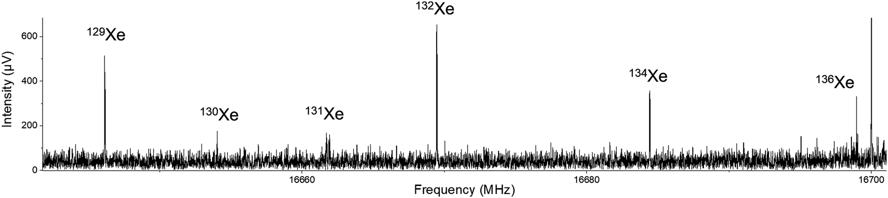 | ||
Fig. 1 The 624 ← 615 transitions for the six most abundant xenon isotopes. The intensity pattern follows the relative abundances of each isotope, with the exception of 131Xe, which is split into nuclear hyperfine components (I131Xe = 3/2). The spike at 16![[thin space (1/6-em)]](https://www.rsc.org/images/entities/char_2009.gif) 700 MHz is a carrier frequency signal. 700 MHz is a carrier frequency signal. | ||
Up to this point, all measurements were made using 1% OCS (Air Products) in pure Xe. To save on the expensive xenon, further measurements were made with a mixture of 1% OCS and 1% xenon in argon. Signals were slightly better in argon expansions than in pure xenon. Backing pressures of 0.7–1.5 bar absolute pressure were used for both carrier gases. With the broadband spectra and assignments as a guide, the sample was brought back to the Coaxially Oriented Beam-Resonator Arrangement (COBRA) spectrometer to complete the measurement of the nine reported isotopologues. The strongest transitions were observed for the μb selection rule, the μa dipole transitions were observed only for the most abundant isotopologues. Fit results of the parent isotopologue are shown in Table 1 where they are compared to selected computational methods. Fits for all isotopologues, including centrifugal distortion constants and inertial defects for the parent species, are included in the ESI.‡
| BLYP | B3LYP | B2PLYP | 132Xe | |
|---|---|---|---|---|
| A 0 (MHz) | 6308.90 | 6450.10 | 6484.08 | 6555.58843(43) |
| B 0 (MHz) | 774.967 | 783.848 | 778.667 | 770.764639(77) |
| C 0 (MHz) | 688.036 | 686.789 | 692.998 | 687.367332(40) |
| N | — | — | — | 131 |
| RMS (kHz) | — | — | — | 1.6 |
3 Computational details
All density functional theory (DFT) calculations are performed using Gaussian,15 using the G09.E01 and G16.A03 revisions. The three density functional approximations (DFAs) used in the current work are chosen to explore the trends in anharmonic vibration–rotation interaction constants (αi) when climbing the “Jacob's ladder” of DFT: they are the generalized gradient approximation BLYP,16,17 the global single hybrid B3LYP,18,19 and the double hybrid B2PLYP.20 All three functionals are always applied with the D3(BJ) empirical dispersion correction,21,22 counterpoise correction,23 and the Dunning-type 3-ζ basis set augmented by diffuse functions,24 with the appropriate effective core potentials (PP) for Xe25 and Hg.26 For the B2PLYP functional, frozen-core approximation is always applied. In the following text, BLYP, B3LYP, and B2PLYP are used instead of the CP-[B,B3,B2P]LYP-D3(BJ)/aug-cc-pVTZ-[PP] notation. Tighter geometry convergence criteria for forces (max. <2 μEh a0−1, RMS <1 μEh a0−1) and displacements (max. <6 μa0, RMS <4 μa0) and a “superfine” (250, 974) grid are applied in all DFT calculations.The anharmonic vibration–rotation interaction constants determined at the coupled cluster level of theory27 for the He, Ne and Ar complexes are calculated using Cfour.28 The basis sets used here are identical to the 3-ζ augmented basis sets used with in the DFT calculations. Frozen-core approximation is always applied. The geometries are optimized with a threshold for RMS of the gradient <10 μEh a0−1. In the following text, CCSD(T) is used instead of the FC-CCSD(T)/aug-cc-pVTZ notation.
The symmetry adapted perturbation theory (SAPT) calculations are performed in Psi429 version 1.3. The SAPT2+(CCD)δMP2 variant is applied with the 3-ζ augmented basis sets, following the recommendation of Parker et al.30 The 5-ζ variants are used as density fitting bases. The rSEe structures based on B2PLYP corrections are used in this set of calculations. In the following text this method is simply called SAPT.
The extrapolated WFT calculations are performed in Psi429 version 1.3rc1 and later. The extrapolation recipe consists of a Hartree–Fock component (HF/cc-pwcV[TQ5]Z), a MP2 component (MP2/cc-pwcV[Q5]Z), and a CCSD(T) correction to the MP2 correlation (ΔCCSD(T)/cc-pwcV[TQ]Z). All correlated levels of wavefunction theory are used with the frozen-core approximation, with density fitting used throughout. The weighted core-valence basis sets31 of 3-, 4-, and 5-ζ quality are used here, with the appropriate effective core potentials (ECP) for Kr, Xe, and Hg atoms. The default auxiliary basis sets for density fitting (up to def2-QZVPPD) are used throughout this work. The extrapolation is performed using the “cubic” Helgaker extrapolation formulas.32 This extrapolation method is called MP2+δ(T) in the following text.
Further corrections are applied to the MP2+δ(T) level of theory in the study of the Xe⋯OCS complex: the all-electron correlation, denoted δAEFC, is estimated by the difference of CCSD(T)/TZP calculations with and without frozen core approximation. To gauge relativistic effects, calculations at the CCSD(T)/TZP-DKH level with the 2nd or 4th order Douglas–Kroll–Hess Hamiltonian are compared to the CCSD(T)/TZP calculations. This correction is denoted δ[2,4]rel, and it is computed using the DKH interface33 in Psi4, with conventional CCSD(T) used instead of the density-fitted variant in the MP2+δ(T) recipe. The TZP-DKH and TZP basis sets are the 3-ζ quality basis sets from Campos and Jorge34 designed for use with and without the Douglas–Kroll–Hess Hamiltonian. Finally, to estimate the effects of diffuse functions on the structure, the aug-cc-pwCV[TQ5]Z basis sets for O, C and S are paired with the cc-pwcV[TQ5]Z-PP basis set for Xe, augmented by diffuse functions from the aug-cc-pV[TQ5]Z-PP basis sets. The results of this calculation are denoted as aug-MP2+δ(T).
All r0, rSEe, and r([1,2])m structures are fit directly to the rotational constants using STRFIT35 version 8a.X.2016.36 All Gaussian, Cfour, and Psi4 input/output files are included in the ESI.‡
4 Results and discussion
4.1 Semi-experimental structures with DFT corrections
The experimental rotational constants at the vibrational zero-point level (B0) can be used to determine a vibrationally averaged ground state structure (r0). Assuming the OCS monomer remains rigid upon complexation with a rare gas atom, the C⋯Rg distance and O–C⋯Rg angle are enough to determine the structure by fitting the measured rotational constants. The same process can be applied to rotational constants, that are corrected towards their equilibrium counterparts (Be). A semi-experimental correction uses the anharmonic vibration–rotation interaction constants αi to calculate the vibrational corrections ΔBDFTe from eqn (1).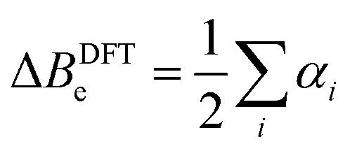 | (1) |
| B0 = Be + ΔBDFTe | (2) |
In principle, both electronic and vibrational effects should be considered in the ΔBe terms. However, the electronic contribution to the ΔBDFTe corrections is in the kHz range for the OCS complexes,13 well within the uncertainty of the vibrational correction. Therefore, we have omitted it in this work. As in our previous investigation,13 the r0 and rSEe structures are fitted to the rotational constants along the a and c axes. The planar structure of the complexes means the rotational constants are correlated, and the inclusion of the third constant would lead to a decreased quality of the fit. It could be argued, that all experimentally available information should be used in the fit, and that any associated decrease in the quality of the fit reflects the errors in either the ΔBDFTe or the fit itself. We have considered this issue, and prefer to remain consistent with previous work. As mentioned above, the equilibrium structure of the OCS monomer is kept rigid and linear. The bond lengths of Morino and Matsumura1 are used for all r0 and rSEe structures.
Unlike in the previous work, the initial fit reported here takes into account all available isotopologue data.|| The resulting rSEe structures obtained with B2PLYP corrections are shown in Fig. 2. The structures obtained using B3LYP and BLYP are listed in the ESI.‡
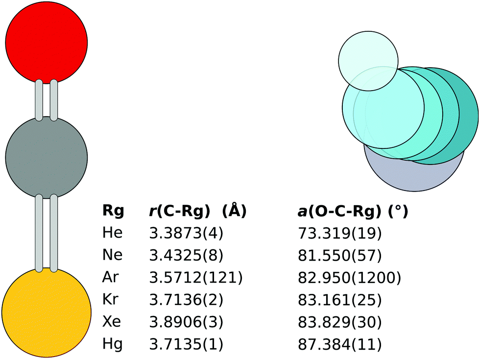 | ||
| Fig. 2 The rSEe structures of the six OCS complexes obtained with B2PLYP corrections. Note: the r(C–Ar) with the 18O isotopologue excluded is 3.5598(3) Å. | ||
The monomer separation increases down the rare gas group. The O–C⋯Rg angle increases with increased molecular weight of the Rg atom. An exception is the Hg⋯OCS complex, which has a monomer separation comparable to the Kr complex, despite the Hg atom being significantly heavier than Kr and even Xe. This shorter distance hints at a different bonding mechanism in the complex.
For the heavier complexes, the rSEe structures obtained with B2PLYP, B3LYP, and BLYP are comparable. This lends confidence to the quality of the structures. In Hg⋯OCS the B2PLYP structure differs from B3LYP and BLYP by less than 3 mÅ, attributed to the different ΔBDFTe along the c axis (1.2 vs. 2.1 and 2.2 MHz, respectively). For Xe⋯OCS the three structures agree within 1 mÅ. The largest relative deviation in the obtained rotational constants is observed for the A rotational constant, as shown in Table 1. In the case of Kr⋯OCS the B3LYP structure differs by 7 mÅ from the other two due to an outlier in ΔBDFTe along the A axis for the parent isotopologue.
In Ar⋯OCS, the B2PLYP-based ΔBDFTe results are affected by an inconsistency in the 18O isotopologue, for which the corrections to B0 and C0 are opposite in sign compared to the parent isotopologue (see ESI‡).13 Hence the somewhat large error in the bond length shown in Fig. 2. A CCSD(T) calculation of the parent isotopologue produces vibration–rotation interaction constants in line with the B3LYP and B2PLYP results. With the 18O isotopologue excluded from the B2PLYP-based fit, the B3LYP and B2PLYP structures agree to 1 mÅ with r(C⋯Ar) = 3.5598(3) for the B2PLYP variant.13 This structure is used as the rSEe in the following text. The BLYP functional predicts a 43 mÅ longer separation.
In the lightest two complexes, some of the DFAs yield negative frequencies when anharmonic corrections are applied to the (positive) harmonic frequencies. Two negative frequencies can be observed in the BLYP results for Ne⋯OCS, one can be observed in both B2PLYP and B3LYP results for the He⋯OCS complex. The weakly bound intermonomer mode is always one of those problematic degrees of freedom. For the Ne⋯OCS complex the B2PLYP and B3LYP corrections are comparable and the rSEe structures differ by less than 3 mÅ. However, the CCSD(T) results for the parent isotopologue are inconsistent with the DFT calculations.
The story is similar in the He⋯OCS complex. The B2PLYP-based rSEe follows the trend in bond lengths of the rare gas group, but the obtained angle is significantly different. On the other hand, the anharmonic frequencies obtained with BLYP do not have negative artefacts, and the angle in the BLYP structure of the He complex is more consistent with the rest of the dataset. However, the intermonomer separation obtained with BLYP is 3.7514(3) Å, which is longer than Kr⋯OCS and therefore unrealistic. The CCSD(T) structure has an angle similar to the BLYP structure, but the intermonomer separation of 3.233 Å is too short, even shorter than the B2PLYP result. Furthermore, the vibration–rotation interaction constants for the parent isotopologue are completely different between the CCSD(T) and the three DFAs. Therefore, the presented rSEe structures for the He and Ne complexes are unreliable.
4.2 Binding and interaction energies
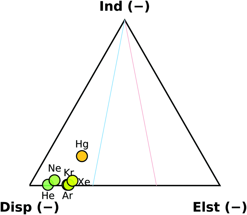
The overall binding energy of a complex (DE) can be defined as the experimentally observable change in the energy upon binding of the monomers. Ignoring basis set and size consistency errors, it can be thought of as the difference of the zero-point corrected energy of the complex from the sum of the zero-point corrected energies of the relaxed monomers. Alternatively, it can be thought of as a sum of the interaction energy (Eint), the deformation energy (ΔED) and the change in the zero-point energy (ΔEZPE). The interaction energy is widely used as a benchmark quantity for computational methods, as calculating Eint requires no geometry optimisation, but just a handful of single-point energy calculations.As a first look on the trends in the interaction energies in this set, we have applied the SAPT decomposition to the B2PLYP-based rSEe geometries. The contribution of the SAPT components of the interaction energy is shown in Fig. 3. The interaction with the rare gases is completely dispersion dominated, with electrostatic contribution increasing slightly down the group. The trend can be attributed to an increasing polarisability of the atoms (1.38, 2.66, 11.08, 16.78, 27.32, and 33.91 a.u. for He, Ne, Ar, Kr, Xe, and Hg, respectively38). The sole exception is the non-rare gas Hg⋯OCS complex, where the interaction contains a significant induction contribution. The second-order E(20)ind,r(A ← B) induction terms are responsible for this behaviour. In the rare gas complexes, the E(20)ind,r(Rg ← OCS) and the E(20)ind,r(OCS ← Rg) terms are approximately equal, while in Hg⋯OCS, the E(20)ind,r(Hg ← OCS) term is ∼10× higher than E(20)ind,r(OCS ← Hg). At infinite separation, these contributions would be determined by the polarisation of A in the unperturbed static multipole of B.39 As shown above, the difference in the static polarisability of Xe and Hg is smaller than between Kr and Xe, therefore this behaviour must have a different cause: at finite separations, the polarisation propagators of the monomers become important.39 It has been previously shown, that a simple electrostatic model is able to reproduce the induced dipole in the Rg⋯CO2 series, while it fails for Hg⋯CO2.40 In the OCS complexes, the predicted dipole moment along the Rg⋯C direction decreases along the group from 0.33 Debye for He down to a minimum of ∼0.17 Debye in the Kr and Xe complexes. In Hg⋯OCS the calculated dipole moment is higher again at 0.28 Debye. We attribute this behaviour to the empty p-orbitals on Hg, which enable additional flexibility in the polarisation of the system compared to the noble gas complexes.
 | ||
| Fig. 3 SAPT decomposition of the interaction energies of the six studied OCS complexes. Energies obtained at the rSEe structures. | ||
The SAPT interaction energies are compared to the counterpoise-corrected MP2+δ(T) interaction energies at the optimized geometries in Table 2. Literature counterpoise-corrected CCSD(T)/aug-cc-pVTZ values of Eint for the Ne8 and Ar41 complexes, along with a CCSD(T)/aug-cc-pVQZ value for the He42 and Kr complexes43 are also shown in Table 2. For the lighter two complexes, the literature values are in a great agreement with our SAPT results. This is not surprising as the geometries used by Feng et al.43 are not too different from our rSEe's. However, our MP2+δ(T) results differ significantly from the other results. For the Ne⋯OCS complex the significantly different geometry (∼0.1 Å) is a likely cause. For the other complexes, the use of the 3-ζ basis sets in the literature and SAPT data introduces a basis set incompleteness error. The MP2+δ(T) values reported here should be of significantly higher accuracy: the energies are calculated at the respective fully-relaxed minima, and the correlation is obtained from larger basis sets, as well as extrapolated towards the complete basis set limit.
| Complex | SAPT | Lit. CCSD(T) | MP2+δ(T) | Experiment | |
|---|---|---|---|---|---|
| E int @ rSEe | E int | E int @ re | D E @ re | D E @ r0 | |
| He⋯OCS | −0.510 | −0.519 | −0.478 | −0.035 | −0.152 |
| Ne⋯OCS | −0.964 | −0.975 | −0.709 | −0.381 | −0.518 |
| Ar⋯OCS | −2.491 | −2.653 | −2.434 | −2.007 | −1.943 |
| Kr⋯OCS | −3.079 | −3.249 | −3.314 | −2.871 | −2.536 |
| Xe⋯OCS | −3.665 | — | −4.025 | −3.827 | −3.158 |
| Hg⋯OCS | −5.015 | — | −4.570 | −4.148 | −3.157 |
A set of experimental estimates of the binding energy is obtained from experimental rotational constants (B, C) and is also shown in Table 2. A diatomic approximation is used to estimate the force constant between the two monomers (ks) from the centrifugal distortion constant (eqn (3)). Then this force constant is used to fit a Lennard-Jones model (eqn (4)).44
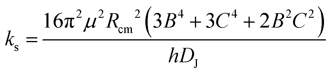 | (3) |
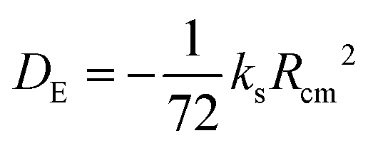 | (4) |
Such experimental binding energies are generally valid under two assumptions: (i) the center-of-mass axis of the monomers is approximately parallel with the a axis of inertia, and (ii) the centrifugal distortion is mainly due to a single vibrational mode along the center-of-mass axis. While the latter is true for all of the studied complexes, the former approximation is only valid from Ar⋯OCS down the group. The agreement between the experimental estimates and the calculated DE data is remarkably good for the rare gas complexes (within “chemical accuracy” of 0.4 kJ mol−1), given how naïve such a fit to a Lennard-Jones model is. The Hg⋯OCS complex is again an outlier: the experimental binding energy is significantly weaker than the calculated value. Relativistic effects are likely to play a significant role in both Hg and Xe complexes. Such effects are “included” implicitly in the experimental value, but in MP2+δ(T) they are treated only in the ECP of the basis set. See further remarks on relativistic effects below. For Hg⋯OCS, a rough estimate of the relativistic effects in the interaction energy can be obtained at the MP2+δ(T) level by replacing the 60-electron relativistic ECP by a 60-electron non-relativistic one. The non-relativistic Eint of −2.918 kJ mol−1 is 1.562 kJ mol−1 lower than the result with the relativistic ECP. The better agreement with the experimental value is likely purely coincidental. For Xe⋯OCS, we had to resort to an estimate using CCSD(T) with all-electron [TQ]ZP and [TQ]ZP-DKH basis sets34 used with and without second order Douglas–Kroll–Hess Hamiltonian, respectively. The non-relativistic Eint is 1.306 kJ mol−1 lower than the relativistic one, similar in magnitude and direction to the Hg⋯OCS case.
The Lennard-Jones model can be in principle cross-checked for validity using calculated data. This is achieved by using the Rcm's from the rB2PLYPe structures, along with the associated rotational constants, as well as the centrifugal distortion constant DB2PLYPJ obtained using second-order vibrational perturbation calculations. The results are shown in Table S12 in the ESI.‡ The binding energies obtained using the supermolecular approach (i.e. from Ecomplex − ∑Emonomers) should be identical to the Lennard-Jones model when B2PLYP-derived data is used in both. The large discrepancy between the rB2PLYPe results and all other results is due to the significant underprediction of the centrifugal distortion constants: for instance, in the He⋯OCS complex, B2PLYP and second-order vibrational perturbation theory predict a DB2PLYPJ of 79.05 kHz, while the experimental value is 438.63 kHz.
Predicting accurate centrifugal distortion constants is a difficult task. In diatomics, the predicted DJ's from wavefunction theory (CCSD(T)/aug-cc-pVTZ) and density functional theory (B3LYP/aug-cc-pVTZ) are comparable, within 10% of experimental values.46 The agreement worsens significantly for the polyatomic CH2PCl: CCSD(T)/cc-pVQZ results are within 25% of the experiment, while upon application of second-order vibrational perturbation theory, or single-hybrid DFAs, the deviation from experiment increases.47 Therefore, the disagreement between the binding energies from the supermolecular and Lennard-Jones approach reflects the innacurate DB2PLYPJ as opposed to an invalidity of the Lennard-Jones model.
The deformation energies for all complexes are negligible when compared to the overall binding energies. In the rare gas complexes, the OCS deformation energies are in the 1–3 J mol−1 range. For these complexes, the O–C–S angle bends towards the rare gas atom by at most 0.2°. In the Hg⋯OCS the deformation energy is slightly higher at 18 J mol−1, and the O–C–S bend reaches 0.3°. While it would seem that the deformation of the OCS monomer increases with increasing binding energy, this is not true for OCS complexes in general. The CS2⋯OCS complex has an interaction energy of ∼8 kJ mol−1, but the OCS molecule is deformed by less than 0.1° at a similar level of theory.48 The zero point energy differences show no particular trends, with the lowest difference calculated for Xe⋯OCS (0.196 kJ mol−1) and the highest for He⋯OCS (0.442 kJ mol−1).
4.3 Interaction energy surfaces
An interaction energy surface of the He⋯OCS dimer calculated with SAPT is shown in Fig. 4. The energy surfaces of the other dimers differ only quantitatively. The two adjusted parameters are the C⋯Rg distance and S–C⋯Rg angle. The OCS monomer was held at the equilibrium bond length.1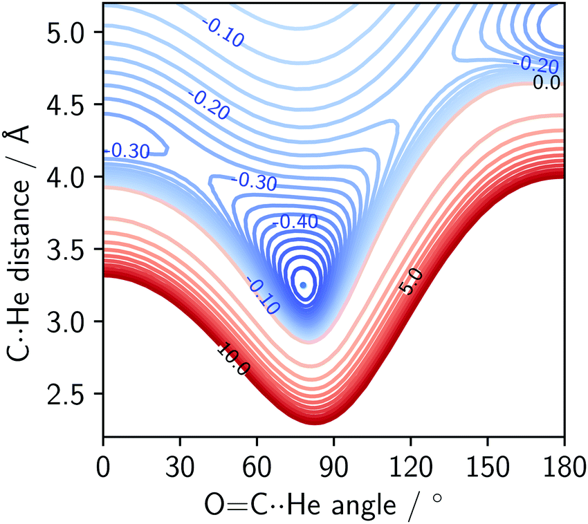 | ||
| Fig. 4 SAPT interaction energy surface of the He⋯OCS complex. Energies in kJ mol−1. Blue contours represent binding (spacing 0.025 kJ mol−1), red represent repulsion (spacing 1 kJ mol−1). | ||
The potential surface of the He complex contains the global minimum, as well as two local minima: the linear conformations He⋯SCO and SCO⋯He. The sulphur-bound conformer is more strongly bound of the two, with an interaction energy of ∼70% of the global minimum. The oxygen-bound conformer is more weakly bound, and for heavier complexes (Kr onwards) this stationary point becomes a transition state. The SAPT surfaces show the same features as the potential surfaces of He,42 Ne,8 Ar,41 and Kr⋯OCS43 complexes. The shape of the potential surface near the global minimum is extremely flat and asymmetric. In fact, for the He⋯OCS species with a calculated DE of −35 J mol−1 (at 0 K, see Table 2), it is surprising an experimental observation of the complex was possible at all.
4.4 Mass-dependent structures of Xe⋯OCS and Ne⋯OCS
An appealing alternative to the semi-experimental method for obtaining near-equilibrium structures is the mass-dependent approach of Watson.49 As above, the equilibrium moments of inertia (Ie) can be obtained from the experimental moments of inertia at the vibrational ground state (I0) and a vibrational zero-point correction (ε0). In a departure from the semi-experimental treatment, in the mass-dependent structures the vibrational corrections are fitted to experimental data according to eqn (5).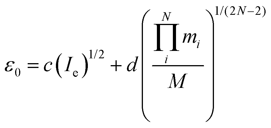 | (5) |
With a measurement of 9 isotopologues of Xe⋯OCS, it is possible to fit the 5 structural parameters required to fully define the structure of the planar complex, as well as the c and d coefficients. The fitted parameters are the C⋯Xe, CO, and CS lengths, and the O–C⋯Xe, and O–C–S angles. Additionally, the full set of cα's as well as dA and dB are fitted. The dihedral angle, as well as dC, are not fit to ensure planarity. In total, 10 parameters are fitted to the 27 rotational constants to obtain the r(2)m structure of Xe⋯OCS. The r(1)m structure was obtained analogously.
The only significant difference between the two mass-dependent structures is in the OC bond length. In the r(2)m structure the bond is 20 mÅ longer than the equilibrium distance of OCS. In the r(1)m the difference is only 10 mÅ. When the OC bond is held fixed to the shorter equilibrium bond length in OCS, the remaining structural parameters (OCS angle, CS bond length and the Xe-dependent parameters) remain within the uncertainty of the fits and the degree of fit decreases slightly. Both rm structures also show a bend in the OCS monomer of ∼1°. From this data alone it is impossible to judge whether the distortion of the OCS monomer is an artefact of the fit.
The most striking difference between the r(2)m and rSEe structures is in the 30 mÅ shorter C⋯Xe distance in the mass-dependent structure (see Fig. 5, as well as Fig. 2 for the rSEe structural parameters). The 1.3° higher O–C⋯Xe angle is mainly due to the 1.1° bend of the OCS unit from a linear shape. The intermonomer potential in the r(2)m structures is shifted slightly towards the S atom.
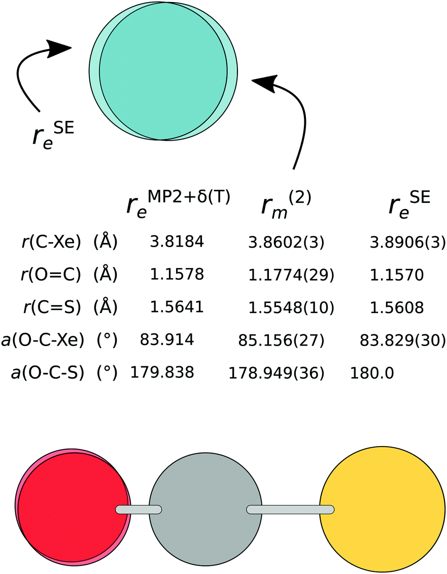 | ||
| Fig. 5 The semi-experimental (rSEe), mass-dependent (r(2)m), and theoretical (rMP2+δ(T)e) structure of Xe⋯OCS. | ||
A comparison with the equilibrium structure obtained using MP2+δ(T) reveals that the chosen level of wavefunction theory predicts a significantly shorter monomer separation compared to the mass dependent as well as the semi-experimental structures (by 43 mÅ and 73 mÅ, respectively). The OC⋯Xe angle from MP2+δ(T) is almost identical with the rSEe structure. The OCS monomer in the rSEe structure is only slightly distorted from the equilibrium values, with a 0.2° inward bend. This leads us to two conclusions: (i) the OCS monomer remains at near-equilibrium values, and the significant deviations of the OCS moiety from its equilibrium shape in both rm structures can be attributed to the fitting process, and (ii) an effect unaccounted for in the MP2+δ(T) method leads to a larger monomer separation in the experimental results.
As 7 isotopologues of the Ne⋯OCS complex have been measured by Xu and Gerry,6 it is possible to apply the above fitting process to that set of rotational constants. The resulting r(2)m structure is compared to the rSEe structure with B2PLYP-based corrections and the rMP2+δ(T)e structure in Fig. 6.
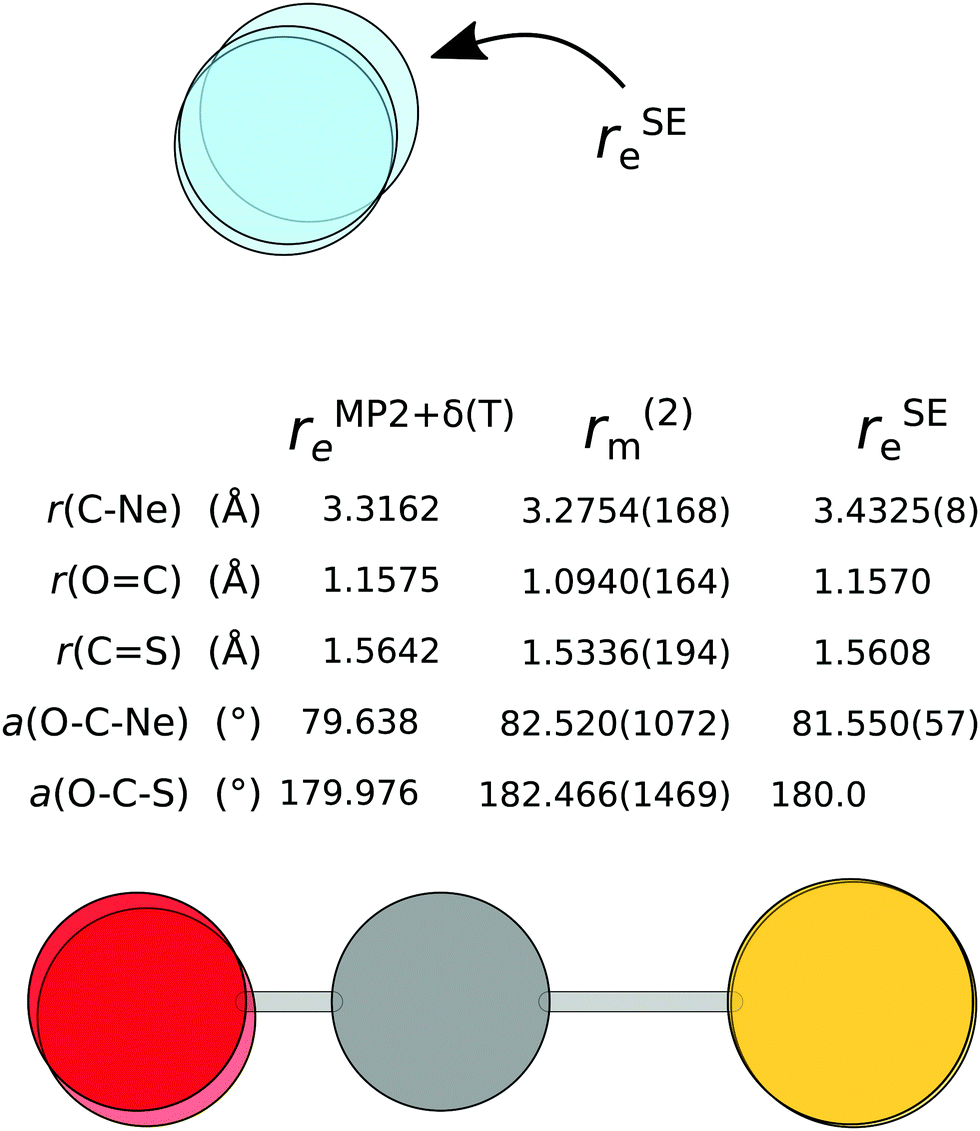 | ||
| Fig. 6 The semi-experimental (rSEe), mass-dependent (r(2)m) and theoretical (rMP2+δ(T)e) structure of Ne⋯OCS. | ||
The issues with the rSEe structure are obvious at the first glance: the C⋯Ne distance is longer by ∼140 mÅ compared to the other two structures, and the angle is also significantly different. As a very similar rSEe structure has been obtained with B3LYP-based corrections, this inaccuracy is unlikely due to the DFA itself, but more likely a failure of the vibrational perturbation theory for such shallow modes. The frequency shift of the C⋯Ne stretch into the imaginary region upon anharmonic correction supports this argument.
There are significant differences in the r(2)m and rMP2+δ(T)e structures. The position of the O-atom in the r(2)m structure is troublesome, despite including the 18O isotopologue in the fit. At 1.094 Å, the OC bond is unphysically short, and the O–C–S angle is over 180°, meaning the OCS molecule deflects away from the Ne atom. Unfortunately, fixing individual OCS parameters leads to a much poorer fit. When the OC distance is fixed to the equilibrium value, the structure fit doesn't converge, unless both CS length and O–C–S angle are also fixed. The best option seems to be to fix the O–C–S angle to 180°. This forces the OC bond to shrink even further, but brings the C⋯Ne bond length within 14 mÅ of the MP2+δ(T) value. Finally, while the d-contributions in the r(2)m fit are associated with a large uncertainty, simply removing them doesn't alleviate the issues with the structure. The r(1)m and r(2)m structures are essentially identical.
4.5 Chasing experimental accuracy with wavefunction theory
The MP2+δ(T) recipe contains a Hartree–Fock component calculated from a [3,4,5]-ζ extrapolation. The correlation energy is calculated from two components: a second-order Møller–Plesset component calculated in an extrapolated [4,5]-ζ basis, and a higher-order correlation correction obtained from a difference in CCSD(T) and MP2 energies in an extrapolated [3,4]-ζ basis.The Hartree–Fock component is likely to be converged to the complete basis set limit.51 The convergence of the correlation energy is not so certain, and can be improved in three ways: (i) by calculating correlation at a higher level of theory, (ii) by using a larger basis set or adding diffuse and/or midpoint functions, or (iii) by correlating all electrons in the calculation. Higher level correlation in dispersion-dominated complexes of similar interaction energies was studied by Řezáč and Hobza:52 the CCSDT(Q) correction to a CCSD(T) energy accounts for only 1–3% of the interaction energy. Due to the enormous computational cost of CCSDT(Q) calculations, we currently cannot investigate higher order effects on this system.
Basis set incompleteness at the CCSD(T)/[3,4]-ζ level is about ∼50 mÅ in the very weakly bound Ar⋯Ar complex, and decreases to ∼5 mÅ for a more strongly bound complex, such as NH3⋯HF.53 The effect of increasing basis set size in the δ(T) component of the MP2+δ(T) recipe is shown in Fig. 7, in the left panel. Note that the OC⋯S angle in the r(2)m structure ( ) is adjusted here by assuming the OCS monomer is linear. With increasing basis set size (
 ), the intermonomer distance hardly changes, and the main difference is in the OC⋯Xe angle. This further confirms that the structure is likely near convergence with respect to basis set size.
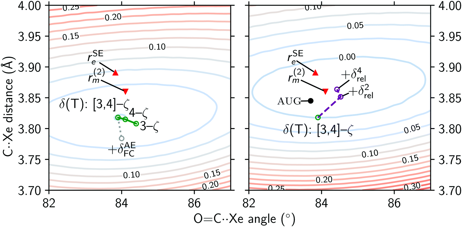 | ||
| Fig. 7 The potential energy surface of Xe⋯OCS. Left: The MP2+δ(T) surface overlaid with points showing the effect of increasing basis set size (green) and the all electron correction (gray) on the structure. Right: The MP2+δ(T) + δrel4 surface overlaid with points showing increasing order in the DKH Hamiltonian (purple). The results of the calculation with additional diffuse functions in the basis sets (aug-MP2+δ(T)) are also shown (black). Points corresponding to the semi-experimental and mass-weighted structure (red) are included for comparison. Contours correspond to energies above the MP2+δ(T) minimum, in kJ mol−1. | ||
We have investigated two additional basis set effects: counterpoise correction for the basis set superposition error, and the effect of diffuse functions. The former has no significant effect on the structure, as the difference in the monomer separation obtained from MP2+δ(T) and CP-MP2+δ(T) is only 0.001 Å. On the other hand, the aug-MP2+δ(T) structure obtained with cc-pwCV[TQ5]Z basis sets augmented by diffuse functions (see in Fig. 7) is remarkably close to the experimental r(2)m structure, with a disagreement in the monomer separation of only 15 mÅ. While this is most certainly a step in the right direction, the increased computational cost compared to cc-pwCV[TQ5]Z calculations is immense: the augmentation of the basis set increases the number of basis functions by 20%, and the amount of memory required for the computation of the connected triples (i.e. the (T) component) more than doubles. Notably, additive terms obtained from the differences of augmented and unaugmented 3-ζ calculations that are used in various extrapolation recipes do not perform well for non-covalent complexes.53,54 Therefore CCSD(T) computations with augmented 4-ζ basis sets might be unavoidable. Unfortunately, the currently available set of “aug-cc-pwCVnZ”-quality basis sets is limited to the first two periods in the main group and first row transition metals, and appropriate density fitting basis sets are also unavailable.
When the effect of correlating all core electrons is added to the MP2+δ(T) potential surface ( ), the minimum in the potential moves even further away from the r(2)m and rSEe results. This could be an incompatibility of the cc-pwcV[TQ]Z-PP basis sets used for the frozen-core components with the all-electron TZP basis set used to calculate the δAEFC (as AE-CCSD(T)/TZP – FC-CCSD(T)/TZP). An all-electron 4-ζ CCSD(T) geometry optimisation is currently prohibitively expensive.
On the right panel of Fig. 7 we illustrate the effect relativistic corrections have on the potential energy surface, as well as on the minimum structures. By adding 4-th order corrections using the Douglas–Kroll–Hess Hamiltonian to the MP2+δ(T) potential, we obtain a global minimum that is within 10 mÅ of the r(2)m structure. The OC⋯Xe angle is also essentially the same when a linear OCS is assumed in the r(2)m structure. However, it is worth noting that the relativistic effects are double counted in the right panel of Fig. 7: both scalar as well as spin–orbit effects are incorporated into the Xe effective core potentials,25 the addition of the Douglas–Kroll–Hess correction treats the scalar relativistic effects a second time. These results confirm relativistic effects play an important role in the stabilisation of the Xe⋯OCS complex, but the agreement of the MP2+δ(T) + δrel4 results with the r(2)m structure is a case of obtaining a correct answer for the wrong reasons.
5 Conclusion
We present a (i) systematic computational study of OCS complexes with the noble gas group, (ii) an accurate structure of the Xe⋯OCS complex based on rotational spectroscopic data, and (iii) a detailed investigation into the geometry of the OCS monomer upon complexation.The semi-experimental structures for the He and Ne complexes based on corrections obtained with DFT are unreliable. This is attributed to a suspected breakdown of the second order vibrational perturbation theory for such flat intermolecular potentials. For the complexes of heavier atoms (Ar, Kr, Xe, Hg), the presented rSEe structures are significantly more reliable.
The binding mechanism in the rare gas complexes is dispersion dominated. In the Hg complex a small proportion of induction contributes to the binding, due to the empty p-shell of Hg. The calculated MP2+δ(T) binding energies DE are in a good agreement with the experimental values using the Lennard-Jones model for complexes up to Kr. This agreement breaks down with in heavier complexes likely due to relativistic effects. The minor disagreement in the interaction energies compared to previous CCSD(T) literature data can be explained by basis set incompleteness in the literature results. The deformation of the OCS monomer from its equilibrium structure upon complexation is predicted to be minimal, with the largest bend of 0.3° predicted for Hg⋯OCS.
The mass-dependent r(2)m structures of the Xe and Ne complexes differ significantly from the rSEe structures. The bond lengths and angles in the OCS monomer are distorted in the r([1,2])m fits, especially the position of the O-atom. However, with the OCS monomer constrained to its equilibrium geometry, the mass-dependent structures are likely the most accurate structures ever obtained for the two complexes. The 43 mÅ difference in the monomer separation in the MP2+δ(T) and r(2)m structures can be partially explained by the lack of diffuse functions in the cc-pwcVnZ basis sets: upon augmentation the difference drops to 15 mÅ. The closest agreement with the r(2)m structure could be obtained by adding the 4-th order relativistic correction (+δrel4) to the MP2+δ(T) results, highlighting the importance of relativistic effects. However, this procedure cannot be generally recommended, as the scalar relativistic effects are double-counted. The inclusion of diffuse functions into at least 4-ζ basis sets is a more systematic way of converging towards experimental structures.
Conflicts of interest
There are no conflicts to declare.Acknowledgements
This work was carried out on the Leibniz Universität Hannover compute cluster, which is funded by the Leibniz Universität Hannover, the Lower Saxony Ministry of Science and Culture (NI MWK) and the German Research Association (DFG). PK would like to thank Susi Lehtola for his helpful comments.Notes and references
- Y. Morino and C. Matsumura, Bull. Chem. Soc. Jpn., 1967, 40, 1095–1100 CrossRef CAS.
- H. A. Dijkerman and G. Ruitenberg, Chem. Phys. Lett., 1969, 3, 172–174 CrossRef CAS.
- F. J. Lovas and R. D. Suenram, J. Chem. Phys., 1987, 87, 2010–2020 CrossRef CAS.
- M. Iida, Y. Ohshima and Y. Endo, J. Chem. Phys., 1991, 94, 6989–6994 CrossRef CAS.
- Y. Xu, W. Jäger and M. C. L. Gerry, J. Mol. Spectrosc., 1992, 151, 206–216 CrossRef CAS.
- Y. Xu and M. C. L. Gerry, J. Mol. Spectrosc., 1995, 169, 542–554 CrossRef CAS.
- J. Tang and A. R. W. McKellar, J. Chem. Phys., 2001, 115, 3053–3056 CrossRef CAS.
- H. Zhu, Y. Zhou and D. Xie, J. Chem. Phys., 2005, 122, 2–8 Search PubMed.
- Y. Xu and W. Jäger, J. Mol. Spectrosc., 2008, 251, 326–329 CrossRef CAS.
- J. J. Newby, M. M. Serafin, R. A. Peebles and S. A. Peebles, Phys. Chem. Chem. Phys., 2005, 7, 487–492 RSC.
- Z. Yu, K. J. Higgins, W. Klemperer, M. C. McCarthy, P. Thaddeus, K. Liao and W. Jäger, J. Chem. Phys., 2007, 127, 054305 CrossRef.
- M. Dehghany, J. N. Oliaee, M. Afshari, N. Moazzen-Ahmadi and A. R. W. McKellar, J. Chem. Phys., 2009, 130, 224310 CrossRef CAS PubMed.
- P. Kraus, D. A. Obenchain and I. Frank, J. Phys. Chem. A, 2018, 122, 1077–1087 CrossRef CAS PubMed.
- M. K. Jahn, D. A. Dewald, D. Wachsmuth, J.-U. Grabow and S. C. Mehrotra, J. Mol. Spectrosc., 2012, 280, 54–60 CrossRef CAS.
- M. J. Frisch, G. W. Trucks, H. B. Schlegel, G. E. Scuseria, M. A. Robb, J. R. Cheeseman, G. Scalmani, V. Barone, B. Mennucci, G. A. Petersson, H. Nakatsuji, M. Caricato, X. Li, H. P. Hratchian, A. F. Izmaylov, J. Bloino, G. Zheng, J. L. Sonnenberg, M. Hada, M. Ehara, K. Toyota, R. Fukuda, J. Hasegawa, M. Ishida, T. Nakajima, Y. Honda, O. Kitao, H. Nakai, T. Vreven, J. A. Montgomery Jr., J. E. Peralta, F. Ogliaro, M. Bearpark, J. J. Heyd, E. Brothers, K. N. Kudin, V. N. Staroverov, R. Kobayashi, J. Normand, K. Raghavachari, A. Rendell, J. C. Burant, S. S. Iyengar, J. Tomasi, M. Cossi, N. Rega, J. M. Millam, M. Klene, J. E. Knox, J. B. Cross, V. Bakken, C. Adamo, J. Jaramillo, R. Gomperts, R. E. Stratmann, O. Yazyev, A. J. Austin, R. Cammi, C. Pomelli, J. W. Ochterski, R. L. Martin, K. Morokuma, V. G. Zakrzewski, G. A. Voth, P. Salvador, J. J. Dannenberg, S. Dapprich, A. D. Daniels, Ö. Farkas, J. B. Foresman, J. V. Ortiz, J. Cioslowski and D. J. Fox, Gaussian 09 Revision E.01, 2016, http://www.gaussian.com Search PubMed.
- A. D. Becke, Phys. Rev. A: At., Mol., Opt. Phys., 1988, 38, 3098–3100 CrossRef CAS PubMed.
- C. Lee, W. Yang and R. G. Parr, Phys. Rev. B: Condens. Matter Mater. Phys., 1988, 37, 785–789 CrossRef CAS PubMed.
- A. D. Becke, J. Chem. Phys., 1993, 98, 1372–1377 CrossRef CAS.
- P. J. Stephens, F. J. Devlin, C. F. Chabalowski and M. J. Frisch, J. Phys. Chem., 1994, 98, 11623–11627 CrossRef CAS.
- S. Grimme, J. Chem. Phys., 2006, 124, 034108 CrossRef PubMed.
- E. R. Johnson and A. D. Becke, J. Chem. Phys., 2005, 123, 024101 CrossRef PubMed.
- S. Grimme, S. Ehrlich and L. Goerigk, J. Comput. Chem., 2011, 32, 1456–1465 CrossRef CAS PubMed.
- S. F. Boys and F. Bernardi, Mol. Phys., 1970, 19, 553–566 CrossRef CAS.
- D. E. Woon and T. H. Dunning, J. Chem. Phys., 1993, 98, 1358–1371 CrossRef CAS.
- K. A. Peterson, D. Figgen, E. Goll, H. Stoll and M. Dolg, J. Chem. Phys., 2003, 119, 11099–11112 CrossRef CAS.
- K. A. Peterson and C. Puzzarini, Theor. Chem. Acc., 2005, 114, 283–296 Search PubMed.
- G. D. Purvis and R. J. Bartlett, J. Chem. Phys., 1982, 76, 1910–1918 CrossRef CAS.
- J. F. Stanton, J. Gauss, L. Cheng, M. E. Harding, D. A. Matthews and P. G. Szalay, CFOUR, Coupled-cluster techniques for computational chemistry, 2010, http://www.cfour.de.
- R. M. Parrish, L. A. Burns, D. G. Smith, A. C. Simmonett, A. E. DePrince, E. G. Hohenstein, U. Bozkaya, A. Y. Sokolov, R. Di Remigio, R. M. Richard, J. F. Gonthier, A. M. James, H. R. McAlexander, A. Kumar, M. Saitow, X. Wang, B. P. Pritchard, P. Verma, H. F. Schaefer, K. Patkowski, R. A. King, E. F. Valeev, F. A. Evangelista, J. M. Turney, T. D. Crawford and C. D. Sherrill, J. Chem. Theory Comput., 2017, 13, 3185–3197 CrossRef CAS PubMed.
- T. M. Parker, L. A. Burns, R. M. Parrish, A. G. Ryno and C. D. Sherrill, J. Chem. Phys., 2014, 140, 094106 CrossRef.
- K. A. Peterson and T. H. Dunning, J. Chem. Phys., 2002, 117, 10548–10560 CrossRef CAS.
- A. Halkier, T. Helgaker, P. Jørgensen, W. Klopper and J. Olsen, Chem. Phys. Lett., 1999, 302, 437–446 CrossRef CAS.
- A. Wolf, M. Reiher and B. A. Hess, J. Chem. Phys., 2002, 117, 9215–9226 CrossRef CAS.
- C. T. Campos and F. E. Jorge, Mol. Phys., 2013, 111, 165–171 CrossRef.
- Z. Kisiel, J. Mol. Spectrosc., 2003, 218, 58–67 CrossRef CAS.
- Z. Kisiel, PROSPE – Programs for rotational spectroscopy, Accessed: 2019-03-19, http://info.ifpan.edu.pl/~kisiel/prospe.htm.
- V. Barone, J. Chem. Phys., 2005, 122, 014108 CrossRef PubMed.
- P. Schwerdtfeger and J. K. Nagle, Mol. Phys., 2019, 117, 1200–1225 CrossRef CAS.
- B. Jeziorski, R. Moszynski and K. Szalewicz, Chem. Rev., 1994, 94, 1887–1930 CrossRef CAS.
- C. R. Jacob, T. A. Wesolowski and L. Visscher, J. Chem. Phys., 2005, 123, 174104 CrossRef PubMed.
- H. Zhu, Y. Guo, Y. Xue and D. Xie, J. Comput. Chem., 2006, 27, 1045–1053 CrossRef CAS PubMed.
- J. M. Howson and J. M. Hutson, J. Chem. Phys., 2001, 115, 5059–5065 CrossRef CAS.
- E. Feng, C. Sun, C. Yu, X. Shao and W. Huang, J. Chem. Phys., 2011, 135, 124301 CrossRef PubMed.
- D. J. Millen, Can. J. Chem., 1985, 63, 1477–1479 CrossRef CAS.
- J. K. G. Watson, in Vibrational spectra and structure, ed. J. R. Durig, Elsevier, 1977 Search PubMed.
- M. O. Sinnokrot and C. D. Sherrill, J. Chem. Phys., 2001, 115, 2439–2448 CrossRef CAS.
- W. X. Pang, H. Y. Wu, J. J. Zhao and Y. B. Sun, Phosphorus, Sulfur Silicon Relat. Elem., 2019, 194, 69–75 CrossRef CAS.
- P. Kraus and I. Frank, J. Phys. Chem. A, 2018, 122, 4894–4901 CrossRef CAS PubMed.
- J. K. G. Watson, A. Roytburg and W. Ulrich, J. Mol. Spectrosc., 1999, 196, 102–119 CrossRef CAS PubMed.
- J. K. G. Watson, J. Mol. Spectrosc., 2001, 207, 16–24 CrossRef CAS PubMed.
- A. J. Varandas, Annu. Rev. Phys. Chem., 2018, 69, 177–203 CrossRef CAS PubMed.
- J. Řezáč and P. Hobza, J. Chem. Theory Comput., 2013, 9, 2151–2155 CrossRef PubMed.
- P. Kraus and I. Frank, Int. J. Quantum Chem., 2019, 119, e25953 CrossRef.
- D. A. Obenchain, L. Spada, S. Alessandrini, S. Rampino, S. Herbers, N. Tasinato, M. Mendolicchio, P. Kraus, J. Gauss, C. Puzzarini, J.-U. Grabow and V. Barone, Angew. Chem., Int. Ed., 2018, 57, 15822–15826 CrossRef CAS PubMed.
Footnotes |
| † All computational inputs and outputs, SPFIT and STRFIT files, an overview of isotopologue data, measured transitions, XYZ structures, as well as scripts required to reproduce the figures are attached. See DOI: 10.5281/zenodo.3582270. |
| ‡ Electronic supplementary information (ESI) available. See DOI: 10.1039/d0cp00334d |
| § These authors contributed equally to this work. |
| ¶ COBRA stands for Coaxially Oriented Beam-Resonator Arrangement. |
| || For He⋯OCS: the parent, 13C, and 34S isotopologues;9 for Ne⋯OCS: the parent, 21Ne, 22Ne, 18O, 13C, 33S, and 34S isotopologues;6 for Ar⋯OCS: the parent, 17O, 18O, 13C, and 34S isotopologues;5 for Kr⋯OCS: the 82Kr, 84Kr, and 86Kr isotopologues;3 for Hg⋯OCS: the 198Hg, 199Hg, 200Hg, 201Hg, 202Hg, and 204Hg isotopologues;4 for Xe⋯OCS: the 129Xe, 129Xe34S, 130Xe, 131Xe, 132Xe, 132Xe13C, 132Xe34S, 134Xe, and 136Xe isotopologues. |
| This journal is © the Owner Societies 2020 |