Experimental design and optimisation (5): an introduction to optimisation

Abstract

Once a suitable experimental design has been used to find the most important factors affecting the outcome of an experiment, and maybe to find any significant interactions between them, we can use an optimisation method to find the best levels (values) for those factors. This Technical Brief outlines the basic principles of optimisation, and introduces some of the most commonly used approaches.

---

Previous Technical Briefs (numbers 24, 26, 36,¹ and 55 ²) have shown how it is possible to identify the factors (i.e., experimental variables) that most affect the result of an analytical experiment. Even simple experiments are influenced by quite large numbers of quantitative and possibly qualitative factors, so efficient experimental designs are extremely valuable, and many different methods have been used. The aim is always to obtain the maximum information from the smallest possible number of trial runs: to minimise the number of trials it is normal to change the levels (i.e. values) of several factors between one run and the next. The simplest experimental designs may identify only the main factors: information on any interactions between them usually requires a larger number of trial runs. Designs should also take into account the inevitable random errors, to determine whether an observed change in the outcome of an experiment is significant: analysis of variance (ANOVA) methods provide this information. When we move on to the optimisation process our aims are similar (and indeed some optimisation methods utilise simple factorial designs – see below). We now wish to find the best level for each of a hopefully modest number of the crucial factors we have identified, which may influence the experimental outcome interactively. Our methods should be able to handle such interactions without too many trial experiments. There may be a conflict between getting a truly optimum outcome and minimising the number of trials to save resources; in practice it is often sufficient to get close to the optimum in relatively few trials. Again, random errors must be considered; as we near the optimum, changes in the experimental response with different factor levels will often be comparable with these errors. This may be another practical justification for being content with a small number of trials and a near-optimum outcome.

Starting an optimisation

A crucial first step is to identify exactly the (single) experimental response that we wish to optimise. Sometimes we shall be seeking a maximum response – the fastest reaction rate, the highest spectroscopic emission intensity, and so on. In other cases, the response of interest may be more complex – the best signal : background ratio, for example, or the best chromatographic resolution between two sample components. As always, a failure to define our experimental aim exactly is likely to yield a flawed outcome.

To optimise just a single factor we do not normally need sophisticated methods. Factors such as wavelength, spectral bandwidth, or electrode potential can be altered so readily that their optimisation is trivial. And automatic analysis methods can be adapted to provide gradients in flowing liquid systems so that, for example, the optimum pH for a reaction can be established in what is effectively a single experiment. In the rare cases where one factor with continuous values cannot be studied in one experiment, the best approach is to start with two trials with different levels of the factor, using the results to set the factor levels for the third and subsequent trials, gaining information at each step: details are given in standard texts.³

Optimisation with two (or more) experimental factors is more complex. In adjusting a spectroscopic detector for example the signal to background ratio may depend on the wavelength and the spectral bandwidth. These two factors will probably interact with each other (i.e., the optimum wavelength may depend on the bandwidth and vice versa), so univariate search methods are inappropriate. Optimisation methods are usually illustrated using two-factor examples because simple pictorial representations of the factor space are available. In some cases, a 3-dimensional response surface or “mountain” picture is used. Several response surface approaches to optimisation are available, but perhaps the most useful method for displaying the two-factor situation is a contour diagram (Fig. 1). The contours join points of equal system response: in the figure the optimum is shown by the central point. These graphical displays cannot very easily be extended to cover three or more factors, but the optimisation methods in common use can handle such situations mathematically.

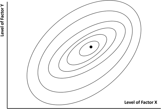Fig. 1 A contour diagram for a two-factor response surface.

At the start of the optimisation process the form of the contours is evidently unknown, while the aim is to approach their centre as expeditiously as possible. To achieve this we have two general options. We could use a carefully designed set of experiments to explore the response within a region of interest, then fit some mathematical model of the response, which we can use to identify a prospective optimum. This approach is called response surface modelling (RSM) and will be discussed in a later Technical Brief. The alternative approach, sometimes called sequential optimisation, is to forgo a model and simply seek an optimum by adjusting the factor levels using information gained in successive experiments. This Technical Brief outlines some of these sequential methods.

An important property of a contour diagram is that it represents the degree of interaction between the two factors. If there is no such interaction the major and minor axes of the roughly elliptical contours would lie parallel to the main axes of the diagram. Then if Factor X was held at a constant level while trials were run with various levels of Factor Y, the optimum value for the latter would be the same at all levels of Factor X: the optimum level for Factor X could similarly be found using any sensible level of Factor Y. This suggests one possible approach to the more likely situation where the factors do interact, the contour axes then being at an angle to the main axes, as in Fig. 1. We could start by keeping Factor X constant and trying various levels of Factor Y. When we found the best level for Y at that particular level of X we could reverse the process, keeping Y constant at its newly-found level and searching for the best X level. By repeating these procedures we would approach the optimum step-wise. This is the iterative univariate or alternating variable search method. It has found little use in analytical work as it is only practicable if the system response can be monitored continuously while the factor levels (e.g., spectrometer wavelengths and bandwidths) are changed easily: otherwise an excessive number of separate experiments is involved.

Another approach that is simple to understand is the method of steepest ascent. We imagine ourselves as standing on the slope of a mountain in a thick fog, while aiming to reach its summit, i.e., the optimum we seek. In real life we would walk in the direction of the steepest slope, taking that to be the quickest way up. So we need information about the local gradient, i.e., the rate of change of response as the factor levels change. In a laboratory experiment we would need a simple factorial design based around our starting point to indicate the direction of steepest ascent. After moving in the indicated direction for a certain distance, ideally checking the response until it starts to fall, we can repeat the factorial design to get fresh information on the steepest route. But even with just two factors each factorial design would require four experiments, so this method also fails the test of minimising the number of trials needed.

The most commonly used method in analytical work when all the factors are continuous variables is simplex optimisation. A simplex is a geometrical figure with one vertex more than the number of factors being studied, so for two factors it is a triangle. The basis of the method is shown in Fig. 2. We begin with three trial experiments with the factor levels given by the points A, B and C. The form of the contours is unknown, but the results show that the worst response is obtained at point A. We reject this point by reflecting it through the line joining B and C to give the position for a single new experiment at point D. There is then a new simplex BCD, with the worst response now at C. This response in turn is rejected by reflection through the line joining B and D, to give another new point E. Continuing this process takes us towards the optimum by means of just one response measurement at each stage, thereby achieving the desired economy of effort. But this simple idea raises a number of questions. How do we decide on the size and position of the initial simplex ABC? When we approach the optimum the rejection-by-reflection process will yield two points alternately, one on either side of the optimum – how do we handle that? How do we calculate the positions of the simplex vertices when there are three or more factors? And how, if at all, does the simplex approach deal with the possibility of subsidiary maxima? These issues will be discussed further in a subsequent Technical Brief.

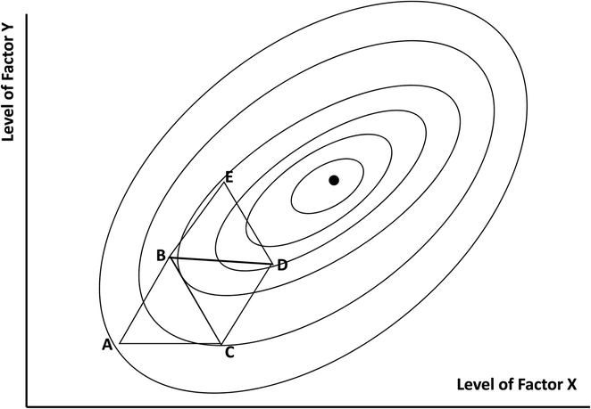Fig. 2 The principle of simplex optimisation.

We have so far assumed that there is a single optimum response that we can locate unequivocally, or at least approach closely. But in some experimental systems this simplification is not justified; there may be local maxima as well as the global maximum (Fig. 3). Such situations may be more common than is generally supposed. A search method should ideally be capable of distinguishing the global response from the lesser local maxima, preferably with a modest number of trial experiments: this significant problem will be discussed in subsequent Technical Briefs.

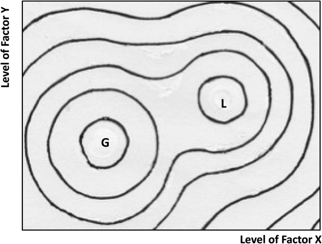Fig. 3 A contour diagram showing global (G) and local (L) maxima.

Some experiments require the optimisation of more than one response simultaneously. In an HPLC separation of compounds 1, 2 and 3 we may wish to optimise the chromatographic resolution of each of the three pairs 1 and 2, 2 and 3, and 1 and 3. Even when only a single factor (e.g., the acetonitrile content of the mobile phase) might affect the experimental outcome, this type of multiple optimisation requires new approaches, again to be discussed in a subsequent Technical Brief.

 

James Miller (Loughborough University)

This Technical Brief was written on behalf of the Statistics Expert Working Group and approved by the Analytical Methods Committee on 25th November 2019.

Further reading

1. AMC Technical Briefs Webpage, https://www.rsc.org/Membership/Networking/InterestGroups/Analytical/AMC/TechnicalBriefs.asp.
2. RSC Publishing Themed Collection, Analytical Methods Committee Technical Briefs, http://rsc.li/amctb.
3. D. L. Massart, et al., Handbook of Statistics and Qualimetrics, Part A, Elsevier, Amsterdam, 1997, pp. 771–774.

---