DOI:
10.1039/C9AY01969C
(Paper)
Anal. Methods, 2020,
12, 112-121
A qualitative recognition method based on Karhunen–Loeve decomposition for near-infrared (NIR) and mid infrared (MIR) spectroscopy analysis
Received
12th September 2019
, Accepted 8th November 2019
First published on 4th December 2019
Abstract
Qualitative recognition is an important research area of NIR and MIR spectroscopy analyses. Feature extraction from the original spectra is the most important step of qualitative analysis for NIR and MIR spectroscopy. In this work, a classification feature extraction method is proposed based on Karhunen–Loeve (K–L) decomposition and the entropy of classification information. Combining the supervised learning method and the extracted features, a qualitative recognition method of NIR and MIR spectroscopy analyses has been proposed. The proposed method has been applied to identify the samples of bamboo pulp fiber, cotton fiber and hemp fiber and also to classify the samples of edible oil. Compared with soft independent modeling of class analogy (SIMCA) based on principal component analysis (PCA) and least squares support vector machines (LS-SVMs) the proposed new method can get better classification results. In the fiber classification test based on NIR spectroscopy analysis, as a linear classification method, SIMCA shows difficulty to classify the overlapping features and only achieves a correct rate of 84.6% (11/13). The nonlinear modeling method LS-SVM improves the accuracy rate to 92.3% (12/13). Our proposed method achieves a 100% (13/13) accuracy rate. In the edible oil classification test based on MIR spectroscopy analysis, in comparison to SIMCA, the proposed method improves the accuracy rate from 59.1% to 77.3%. In both tests, the proposed method demonstrates a better classification and recognition ability.
1 Introduction
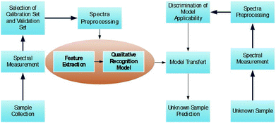
Near-infrared (NIR) and mid-infrared (MIR) spectroscopy analyses are nondestructive detection and rapid analysis methods, which have been widely applied to qualitative recognition and quantitative detection.1–5 The advantage of qualitative recognition based on NIR and MIR spectroscopy analyses is to identify the classification of the samples without knowledge of the contents and components. The process of qualitative recognition based on NIR and MIR spectroscopy analyses is shown in Fig. 1. Qualitative recognition is usually achieved by building a qualitative recognition model based on the chemometric method. Due to the wide range and high resolution of NIR and MIR spectroscopy, the spectra consist of thousands of data and the qualitative recognition model cannot be built directly.6 So the first and most important step is feature extraction, which transforms the original data to feature space. Principal component analysis (PCA) is a popular feature extraction method. Qualitative recognition models are usually built based on the extracted features with various classification methods such as the linear discriminant analysis (LDA),7 soft independent modeling of class analogy (SIMCA),8 least squares support vector machine (LS-SVM),9–11 neural networks (NN)12etc. The widely applied SIMCA methods rely on PCA to extract features from which qualitative recognition models are built. Unknown samples are fitted with all qualitative recognition models, and then the classification is recognized with the F test based on the fitting residuals. The support vector machine (SVM) is a popular and effective nonlinear modeling method.13 Also, to reduce training time and improve the generalization ability, a least squares support vector machine (LS-SVM) has been proposed and applied to the qualitative recognition.14 When the LS-SVM is applied to NIR and MIR spectroscopy analyses,15 the spectral matrix dimension is first reduced by PCA, and then the qualitative or quantitative models are built with the LS-SVM based on dimension reduced data.16
 |
| | Fig. 1 Flow chart of qualitative recognition based on NIR and MIR spectroscopy analyses. | |
A good feature extraction method needs to reduce the data dimension to pursue low computational cost. More importantly, it can convert the original data into a feature space that can finally classify the sample. PCA is proven to be an effective data compression method,17 but, not necessarily an effective feature extraction method.18 The purpose of qualitative recognition based on NIR and MIR spectroscopy analyses is to classify the samples correctly. Usually, the main components of unclassified samples are very similar, such as the fiber samples (from bamboo pulp, cotton and hemp) and the samples of edible vegetable oils. In this case, the large number of principal components could overwhelm the classification information. It is usually difficult to identify the hidden classification information even with the nonlinear classification method.19,20
The Karhunen–Loeve (K–L) decomposition or proper orthogonal decomposition is a method which can represent a stochastic process in terms of the minimum number of degrees of freedom.21,22 They provide a way to extract spatial coherent features from a set of samples.23 K–L decomposition removes the correlation in the original data and achieves minimum variance distortion.24 This work is based on Karhunen–Loeve (K–L) decomposition and the entropy of classification information. Classification features for NIR and MIR spectroscopy analyses are extracted from class mean vectors and class centering eigenvectors. Combined with supervised learning, a novel qualitative recognition method for infrared spectroscopy analysis is proposed. The proposed method has been applied to identify the samples of bamboo pulp fiber, cotton fiber and hemp fiber and also to classify the samples of edible oil. The proposed method generates better classification results than soft independent modeling of class analogy (SIMCA) based on principal component analysis (PCA) and least squares support vector machines (LS-SVMs).25
2 Material and methods
2.1 Spectrometer and experimental parameters
A SupNIR-2700 of Focused Photonics Inc. is used to measure the near infrared diffuse reflection spectra. Samples are scanned 60 times, and the spectral range is 1000–1800 nm, where each sample is tested 10 times. The average is chosen as the sample spectra. The infrared spectra of the edible oil samples are obtained with an ATR-FTIR spectrometer. The spectra were collected from 650 to 4000 cm−1 with a resolution of 4 cm−1. Each sample is scanned three times and the average is used for analysis.
2.2 Dataset
2.2.1 NIR dataset.
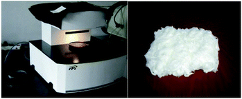
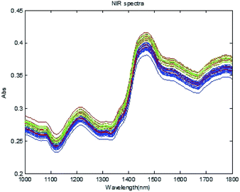
Samples in Fig. 2 are provided by Jigao Chemical Fiber Company, Hebei, China. Fiber samples include bamboo pulp fiber (30 samples), cotton fiber (12 samples) and hemp fiber (10 samples). The original spectra are shown in Fig. 3, where the blue spectra are from bamboo pulp fibers, the red are from cotton fibers and the green are from hemp fibers. To improve the prediction or generalization ability of the qualitative recognition model, an optimal selection method of samples of the calibration set and validation set is applied. The rank-KS optimization method compares variances to select samples with larger differences as test sets.26 Thirteen of the 52 samples are selected as validation sets, including 7 bamboo fiber samples, 3 cotton fiber samples, and 3 hemp fiber samples. The other 39 samples are used as calibration sets (Table 1).27,28
 |
| | Fig. 2 Near-infrared diffuse reflectance spectrometer and samples. | |
 |
| | Fig. 3 Near-infrared spectra of fiber samples. | |
Table 1 Statistics of all rayon samples
| Class |
Bamboo fiber |
Cotton fiber |
Hemp fiber |
| No. of samples |
30 |
12 |
10 |
| No. of calibration set |
23 |
9 |
7 |
| No. of validation set |
7 |
3 |
3 |
| Class no. |
1 |
2 |
3 |
2.2.2 MIR dataset.
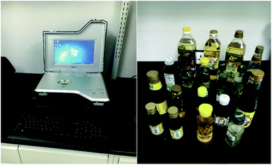
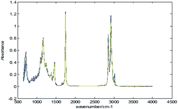
Nine types of edible oil (sesame, corn, canola, blend, sunflower, peanut, olive, soybean, and tea seed) with a total of 84 samples are collected from the National Institute of Metrology (NIM), China. According to ref. 26, 62 samples are for calibration, and the remaining 22 samples are used for validation (Table 2). The samples of edible oil and spectrometer are shown in Fig. 4. The spectra of edible oil samples scanned with an ATR spectrometer are shown in Fig. 5.
Table 2 Statistics of all edible oil samples
|
|
No. |
Total sample number |
Samples in calibration set |
Samples in validation set |
| Sesame oil |
1 |
15 |
12 |
3 |
| Corn oil |
2 |
4 |
3 |
1 |
| Canola oil |
3 |
8 |
5 |
3 |
| Blend oil |
4 |
10 |
8 |
2 |
| Sunflower oil |
5 |
7 |
5 |
2 |
| Peanut oil |
6 |
12 |
9 |
3 |
| Olive oil |
7 |
16 |
12 |
4 |
| Soybean oil |
8 |
7 |
5 |
2 |
| Tea seed oil |
9 |
5 |
3 |
2 |
| Total |
9 |
84 |
62 |
22 |
 |
| | Fig. 4 ATR spectrometer and edible oil samples. | |
 |
| | Fig. 5 MIR spectra of edible oil samples. | |
2.3 Software
All data have been analyzed with MATLAB 2012a (The Mathworks Inc.) and the LS-SVM toolbox (version 1.8).29
2.4 Preprocessing
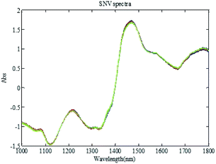
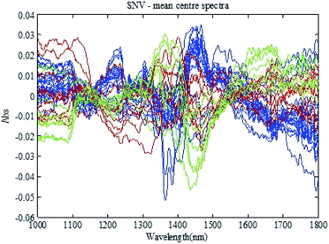
To eliminate the side effects of surface scattering and the change of the optical path on infrared diffuse reflection spectra, standard normal variate transformation (SNV) is first applied to the spectral data. The spectra after SNV are shown in Fig. 6. Spectral mean centering is further applied to eliminate the side effects of the spectral absolute absorption value (shown in Fig. 7).
 |
| | Fig. 6 The NIR spectra with SNV transformation. | |
 |
| | Fig. 7 The NIR spectra with SNV transformation and mean centering processing. | |
2.5 Evaluation of recognition results
The correct classification rate (CCR) is applied to evaluate the qualitative recognition results. CCR is defined as
where n is the total number of samples in the validation set, nic is the number of correct classification samples in class i and k is the total number of classes. Besides qualitative recognition model building, sample selection and model transfer affect the qualitative recognition model application for prediction in the process of qualitative recognition based on NIR and MIR spectroscopy analyses.30,31 Generally, with appropriate model transfer techniques, the qualitative recognition model with a higher correct classification rate (CCR) has a better adaptability to a new experimental dataset. In order to evaluate the classification results of different methods, three indicators are introduced which include sensitivity, precision and specificity. Sensitivity indicates the proportion of positive samples in the samples that are predicted to be correct:
Precision represents the correct quantity in the sample with positive prediction:
Specificity indicates the propotion of negtive classes:
where TP (true positive) indicates the number of samples that are actually positive samples predicted to be positive samples, FP (false positive) indicates the number of samples that are actually positive samples predicted to be negative samples. FN (false negative) indicates the number of samples that are actually negative samples predicted to be negative samples.
3 Theory
3.1 K–L decomposition
K–L decomposition is a feature extraction method for pattern recognition. It decomposes the data matrix Φ to its eigenvalues and eigenvectors as
where Λ is the diagonal matrix eigenvalues of Φ and U is the matrix of eigenvectors of Λ. When Λ is chosen as the covariance matrix, K–L decomposition is equal to principal component analysis (PCA). To extract the classification information from the class mean vectors and the class centering eigenvectors, the within-class scatter matrix Sw and between-class scatter matrix Sb are decomposed with K–L decomposition instead of the covariance matrix in PCA. For classifiers, good feature extraction should not only reduce the data dimension to reduce the amount of computation, but also enhance the ability to select directions to maximize the separation of all known categories. PCA has been proved to be an effective data compression method, but it has shown limitation of feature extraction.32–35 When PCA was used to extract the classification information from the samples with similar components, the classification information could be overwhelmed by other principal components. In this case, it is usually difficult to identify the hidden classification information even with the nonlinear classification method.
3.2 Classification feature extraction from class mean vectors
For a calibration set with k classes of samples (gi samples of each class), the total number of samples is  . The within-class scatter matrix Sw of the spectral matrix X ∈ Rn×m is defined as
The between-class scatter matrix Sb is defined as
where
xij is the
jth spectral vector in class
i,
![[x with combining macron]](https://www.rsc.org/images/entities/i_char_0078_0304.gif) i
i is the mean spectral vector of class
i and

,
![[x with combining macron]](https://www.rsc.org/images/entities/i_char_0078_0304.gif)
is the mean spectral vector of all samples, where

,
Sw ∈
Rm×n,
Sb ∈
Rm×n. If the within-class scatter matrix
Sw is a unit matrix, the unrelated feature of eigenvectors cannot be changed by any orthonormal transformation. Since
Sw is a symmetric and positive definite matrix, K–L decomposition gives
UTSwU =
Λ. Let
B =
UΛ−1/2, then

. Using the transformation matrix B, the between-class scatter matrix

can be used to extract the classification feature from the class mean vectors using K–L decomposition. Assuming that the number of the unrecognized classes is
k, the biggest rank of

is
k − 1 and the corresponding K–L decomposition matrix composed of eigenvectors

is
V′ = [
v1, …,
vk−1]. In general, the transformation matrix is defined as
S =
UΛ−1/2V′, then
| STSwS = Λ′ = (UΛ−1/2V′)T(UΛ−1/2V′) |
According to the eigenvalue matrix Λ′, the d1 eigenvector corresponding to the larger eigenvalue is selected in S to form a transformation matrix W1 ∈ Rm×d1. The classification feature is extracted from the class mean vectors with normalized W1 ∈ Rm×d1 as
where
T1 ∈
Rm×d1, ‖·‖
2 denotes the 2-norm.
3.3 Classification feature extraction from class centering eigenvectors
In addition to class mean vectors, classification features are also reflected in the second order statistical moments. The classification features from the second order statistical moments can be defined by the eigenvectors μi of the within-class scatter matrix Sw. If conditional covariance of one component in the eigenvectors is the same for all classes, the classification feature cannot be extracted from the component. Therefore, the scattering of the conditional covariance in the eigenvectors of the within-class scatter matrix Sw reflects the classification feature. The importance of the classification features in class centering eigenvectors can be measured with the entropy of classification information. For the class j(j = 1, 2, …, n) the eigenvector of the within-class scatter matrix is defined as
and the entropy of classification information J(xi) of the component xi is defined as
where λi is the ith eigenvector of the within-class scatter matrix Sw. If λij concentrates on all classes, J(xi) is small and the uncertainty of classification information is also small. Therefore, J(xi) can be arranged in the following order:
| J(x1) ≤ J(x2) ≤ J(x3) ≤, …, ≤ J(xR) |
d
2 eigenvectors in Sw corresponding to the smallest d2 eigenvalues of Λ′ are chosen to form the feature extraction matrix W2 ∈ Rm×d2. The classification feature is extracted from the class centering eigenvectors with normalized W2 ∈ Rm×d2 as
where
T2 ∈
Rm×d2.
3.4 Classification feature combination
Classification features extracted from class mean vectors and class centering eigenvectors are different. Therefore, it can be combined to form a new transform matrix W ∈ Rm×(d1+d2), where d1 transform vectors are calculated according to description in Section 3.2 and d2 transform vectors are calculated according to description in Section 3.3. The extracted classification features are defined as
where T ∈ Rm×(d1+d2). And averaging the characteristics of each class, the jth feature of the ith class is  .
.
3.5 Sample prediction
The extracted features from K–L decomposition are easy to classify. Classification is achieved by comparing the features of the unknown samples to the features learned from the calibration set. This is the sample prediction process. For the unknown sample matrix Xtest, the classification features are extracted by the transform matrix W as
Prediction for the unclassified samples is based on the Euclidean distance of the extracted classification features as
| tdi = min‖ttest − tendi‖2 |
where
tendi is the extracted classification feature of class
i in the calibration set. The unclassified samples are identified as class
i if the extracted classification feature satisfies the above equation.
4 Results and discussion
For comparison, the same sample set of NIR data is classified by the nonlinear classification method LS-SVM, linear classification method SIMCA and proposed method. And MIR data are classified by the LS-SVM and proposed method.
4.1 NIR data
4.1.1 Qualitative recognition with LS-SVM.
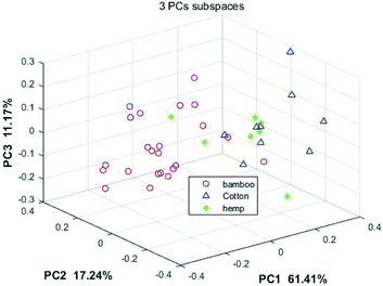
Before building a qualitative recognition model, PCA is used for feature extraction and data compression. The projection of the first three principal components (PCs) into the subspace in the NIR spectrum is shown in Fig. 8, in which 61.41%, 17.24%, and 11.17% are the contribution of the three principals, respectively. It is obvious that the projections of the bamboo fiber, cotton fiber and hemp fiber samples overlap on the principal component subspace; therefore it is difficult to classify even with the nonlinear classification method.
 |
| | Fig. 8 NIR data projected on the subspace for the first 3 of the principal components. | |
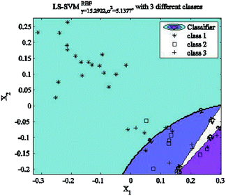
A number of principal components need to be selected when building a qualitative recognition model. Redundant principal components may cause classification interference. On the other hand, insufficient principal components may cause information loss. The classification results with LS-SVM are shown in Fig. 9, where the number of principal components is chosen as 15 and the RBF kernel parameters are chosen as γ = 15.29 and σ2 = 5.14. In Fig. 9, the blue region, the purple region and the pink region represent bamboo, cotton and hemp fiber classes, respectively. Because the extracted classification features based on PCA are overlapping, not all the samples in the validation set can be classified correctly even with 15 principal components. And nonlinear classification methods such as LS-SVM can't achieve good results either. The detailed qualitative recognition results with LS-SVM are shown in Table 3. Clearly, the increasing number of principal components improves the accuracy of qualitative recognition at the beginning. When the number of principal components reaches 6, the accuracy stabilizes at 92.3% (12/13), which means that simply increasing the number of principal components will not always improve the accuracy with LS-SVM.
 |
| | Fig. 9 LS-SVM classification results with 15 principal components. | |
Table 3 Qualitative recognition results by LS-SVM with different principal component numbers
| No. of PC |
γ
|
σ
2
|
Accuracy (%) |
| 3 |
730.76 |
13.69 |
62.9% (9/13) |
| 4 |
1632.74 |
9.534 |
84.6% (11/13) |
| 5 |
91.90 |
1.14 |
84.6% (11/13) |
| 6 |
3.36 |
2.45 |
92.3% (12/13) |
| 7 |
11.89 |
6.60 |
92.3% (12/13) |
| 8 |
569.99 |
48.06 |
92.3% (12/13) |
| 9 |
2282.14 |
68.79 |
92.3% (12/13) |
| 10 |
4516.79 |
3.62 |
92.3% (12/13) |
| 11 |
9.78 |
5.08 |
92.3% (12/13) |
| 12 |
27.53 |
4.69 |
92.3% (12/13) |
| 13 |
499.06 |
6.43 |
92.3% (12/13) |
| 14 |
2.68 |
84 |
92.3% (12/13) |
| 15 |
15.29 |
84 |
92.3% (12/13) |
4.2 MIR data
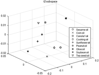
From Sections 3.2 and 3.3, the classification features are extracted from class mean vectors and class centering eigenvectors with K–L decomposition. The extracted classification features are illustrated in Fig. 15. Similarly, features extracted from the same category converge in the extracted feature subspace, while features extracted from different categories are separated from each other. The comparison of the classification results of SIMCA and the proposed method is shown in Table 6. Because PCA extracts the largest direction of data changes and uses lower dimension to represent all data, it focuses more on data compression than feature classification. As the proposed method finds the subspace for classification instead of data compression, it demonstrates a stronger classification ability than SIMCA.
 |
| | Fig. 15 Extracted feature subspace. | |
Table 6 Comparison of the classification results
|
|
Test no. |
Correct no. |
Error no. |
CCR |
| SIMCA method |
22 |
13 |
9 |
59.1% |
| Proposed method |
22 |
17 |
5 |
77.3% |
4.3 Comparison of various parameters of different methods
In order to evaluate the classification results of different methods, three indicators are introduced which include sensitivity, precision and specificity. Three parameters of different categories of samples are shown in Tables 7–11.
Table 7 Three parameters of NIR data in the SIMCA method
| No. |
Sensitivity |
Precision |
Specificity |
| 1 |
100% |
77.8% (7/9) |
66.7% (2/3) |
| 2 |
66.7% (2/3) |
66.7% (2/3) |
90% |
| 3 |
33.3% (1/3) |
100% |
100% |
Table 8 Three parameters of NIR data in the LS-SVM method
| No. |
Sensitivity |
Precision |
Specificity |
| 1 |
85.71% (6/7) |
100% |
100% |
| 2 |
100% |
75% |
90% |
| 3 |
100% |
100% |
100% |
Table 9 Three parameters of NIR data in the proposed method
| No. |
Sensitivity |
Precision |
Specificity |
| 1 |
100% |
100% |
100% |
| 2 |
100% |
100% |
100% |
| 3 |
100% |
100% |
100% |
Table 10 Three parameters of MIR data in the SIMCA method
| No. |
Sensitivity |
Precision |
Specificity |
| 1 |
66.7% (2/3) |
100% |
100% |
| 2 |
100% |
100% |
100% |
| 3 |
66.7% (2/3) |
40% |
82.4% (16/19) |
| 4 |
0% |
0% |
80% |
| 5 |
50% |
50% |
95% |
| 6 |
66.7% (2/3) |
100% |
100% |
| 7 |
50% |
100% |
100% |
| 8 |
50% |
100% |
100% |
| 9 |
100% |
100% |
100% |
Table 11 Three parameters of MIR data in the proposed method
| No. |
Sensitivity |
Precision |
Specificity |
| 1 |
66.7% (2/3) |
100% |
100% |
| 2 |
100% |
100% |
100% |
| 3 |
66.7% (2/3) |
66.7% (2/3) |
94.7% (18/19) |
| 4 |
50% |
25% |
85% |
| 5 |
100% |
66.7% (2/3) |
95% |
| 6 |
100% |
100% |
100% |
| 7 |
50% |
100% |
100% |
| 8 |
50% |
100% |
100% |
| 9 |
100% |
100% |
100% |
5 Conclusions
Qualitative recognition is one of the most important research areas for NIR and MIR spectroscopy analyses. Feature extraction is a crucial step of qualitative analysis. PCA has been proven to be an effective data compression method but fails to extract the important features for classification when the principle component subspace is similar among samples. The main contribution of this work is the proposal of a classification feature extraction method based on Karhunen–Loeve (K–L) decomposition and the entropy of classification information. The proposed method provides a better way to solve these types of qualitative recognition problems based on NIR and MIR spectroscopy analyses. It uses the classification features from both class mean vectors and class centering eigenvectors based on K–L decomposition. The extracted features from the same class converge in the extracted feature subspaces and the ones from different class are separated. This improves accuracy and greatly simplifies the classification step by using simple Euclidean distance criteria. In the fiber classification test based on NIR spectroscopy analysis, as a linear classification method, SIMCA shows difficulty to classify the overlapping features and only achieves a correct rate of 84.6% (11/13). The nonlinear modeling method LS-SVM improves the accuracy rate to 92.3% (12/13). Our proposed method achieves a 100% (13/13) accuracy rate. In the edible oil classification test based on MIR spectroscopy analysis, in comparison to SIMCA, the proposed method improves the accuracy rate from 59.1% to 77.3%. In both tests, the proposed method demonstrates a better classification and recognition ability.
Conflicts of interest
There is no conflict of interest.
Acknowledgements
This work was partially sponsored by financial support from the National Scientific Instrument Major Project of P. R. China (Grant No. 2013YQ220643) and Beijing Natural Science Foundation (4172044).
Notes and references
- E. Teye, X. Huang, H. Dai and Q. Chen, Spectrochim. Acta, Part A, 2013, 114, 183–189 CrossRef CAS PubMed.
- M. K. Ahmed and J. Levenson, Liq. Fuels Technol., 2012, 30, 115–121 Search PubMed.
- A. Ouyang and J. Liu, Meas. Sci. Technol., 2013, 24, 025502 CrossRef.
- R. M. Balabin, R. Z. Safieva and E. I. Lomakina, Anal. Chim. Acta, 2010, 671, 27–35 CrossRef CAS.
- V. Germano, A. D. A. Gomes, D. S. Adenilton Camilo, D. Brito, A. Luiza Bizerra and D. M. Everaldo Paulo, Talanta, 2011, 83, 565–568 Search PubMed.
- C. Lee and D. A. Landgrebe, IEEE Trans. Geosci. Remote Sens., 1993, 31, 792–800 CrossRef.
- M. S. L. Sarabia, Chemom. Intell. Lab. Syst., 1995, 28, 287–303 CrossRef.
- S. Wold and M. Sjostrom, SIMCA: A Method for Analysing Chemical Data in Terms of Similarity and Analogy, ACS Symp. Ser., 1977, 52, 243–282 CrossRef CAS.
- A. N. Xin, X. U. Shuo and L. D. Zhang, Spectrosc. Spectral Anal., 2009, 29, 127 Search PubMed.
- C. J. Burges, Data Min. Knowl. Discov., 1998, 2, 121–167 CrossRef.
-
N. Cristianini and J. Shawe-Taylor, An Introduction to Support Vector Machines, 2000 Search PubMed.
- F. Despagne and D. Massart, Analyst, 1998, 123, 157R RSC.
- R. M. Balabin, R. Z. Safieva and E. I. Lomakina, Microchem. J., 2011, 98, 121–128 CrossRef CAS.
- R. M. Balabin and E. I. Lomakina, Analyst, 2011, 136, 1703–1712 RSC.
- Y. Liu and Y. Zhou, Spectroscopy, 2013, 28, 32–43 CAS.
- A. Candolfi, R. D. Maesschalck, D. L. Massart, P. A. Hailey and A. C. E. Harrington, J. Pharm. Biomed. Anal., 1999, 19, 923 CrossRef CAS.
-
R. C. Gonzalez and R. E. Woods, Digital Image Processing, Prentice Hall International, 2008, vol. 28, pp. 484–486 Search PubMed.
-
A. Cheriyadat and L. Bruce, IGARSS 2003: IEEE International Geoscience and Remote Sensing Symposium, Proceedings: Learning from Earth's Shapes and Sizes, 2003, vol. I–VII, pp. 3420–3422 Search PubMed.
- M. V. Reboucas, J. B. D. Santos, D. Domingos and A. R. C. G. Massa, Vib. Spectrosc., 2010, 52, 97–102 CrossRef CAS.
- M. Blanco and I. Villarroya, TrAC, Trends Anal. Chem., 2002, 21, 240–250 CrossRef CAS.
- L. Sirovich and M. Winter, Phys. Fluids A, 1990, 2, 127–136 CrossRef CAS.
-
M. Loeve, Probability Theory, 1955 Search PubMed.
- M. D. Graham and I. G. Kevrekidis, Comput. Chem. Eng., 1996, 20, 495–506 CrossRef CAS.
- D. Zheng and K. A. Hoo, Comput. Chem. Eng., 2004, 28, 1361–1375 CrossRef CAS.
- X. Ma, A. F. Vakakis and L. A. Bergman, J. Sound Vib., 2008, 309, 569–587 CrossRef.
- W. L. Z. Yuan, Spectrosc. Spectral Anal., 2014, 34, 947–951 Search PubMed.
- Y. Roggo, C. Roeseler and M. Ulmschneider, J. Pharm. Biomed. Anal., 2005, 36, 777–786 CrossRef.
- M. Fontalvo-Gomez, J. A. Colucci, N. Velez and R. J. Romanach, Appl. Spectrosc., 2013, 67, 1142–1149 CrossRef CAS PubMed.
-
K. D. Brabanter, P. Karsmakers, F. Ojeda, C. Alzate, J. D. Brabanter, K. Pelckmans, B. D. Moor, J. Vandewalle and J. A. K. Suykens, LS-SVMlab toolbox user's guide, Ku Leuven Leuven, 2010, vol. 66, p. xix Search PubMed.
- L. Chen, Z. Zhong, C. Yuting and Y. Hongfu, Chemom. Intell. Lab. Syst., 2017, 37, 1587–1594 Search PubMed.
- L. Chen, H. F. Yuan, Z. Zhong, C. F. Song and J. J. Wang, Chemom. Intell. Lab. Syst., 2016, 153, 51–57 CrossRef.
-
R. C. Gonzalez and P. Wintz, Digital image processing, 2007 Search PubMed.
- R. E. Miguel, R. S. Dungan and J. B. R. Iii, J. Anal. Appl. Pyrolysis, 2014, 107, 332–335 CrossRef CAS.
- H. Li, F. R. V. D. Voort, A. A. Ismail, J. Sedman, R. Cox, C. Simard and H. Buijs, J. Am. Oil Chem. Soc., 2000, 77, 29–36 CrossRef CAS.
- J. I. Hong Yang and M. M. Paradkar, Food Chem., 2005, 93, 25–32 CrossRef.
|
| This journal is © The Royal Society of Chemistry 2020 |
Click here to see how this site uses Cookies. View our privacy policy here.  a,
Wei
Liu
a,
Hongfu
Yuan
a,
Wei
Liu
a,
Hongfu
Yuan
 b and
Chunfeng
Song
b
 . The within-class scatter matrix Sw of the spectral matrix X ∈ Rn×m is defined as
![[x with combining macron]](https://www.rsc.org/images/entities/i_char_0078_0304.gif) i is the mean spectral vector of class i and
i is the mean spectral vector of class i and  ,
, ![[x with combining macron]](https://www.rsc.org/images/entities/i_char_0078_0304.gif) is the mean spectral vector of all samples, where
is the mean spectral vector of all samples, where  , Sw ∈ Rm×n, Sb ∈ Rm×n. If the within-class scatter matrix Sw is a unit matrix, the unrelated feature of eigenvectors cannot be changed by any orthonormal transformation. Since Sw is a symmetric and positive definite matrix, K–L decomposition gives UTSwU = Λ. Let B = UΛ−1/2, then
  . Using the transformation matrix B, the between-class scatter matrix
  can be used to extract the classification feature from the class mean vectors using K–L decomposition. Assuming that the number of the unrecognized classes is k, the biggest rank of
  is k − 1 and the corresponding K–L decomposition matrix composed of eigenvectors
  is V′ = [v1, …, vk−1]. In general, the transformation matrix is defined as S = UΛ−1/2V′, then
 .
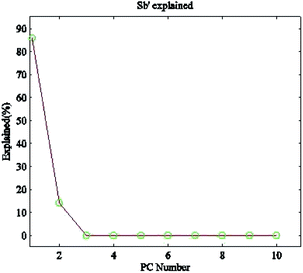
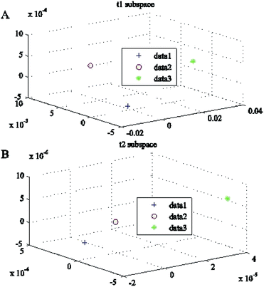
.
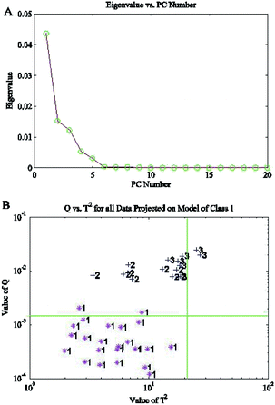
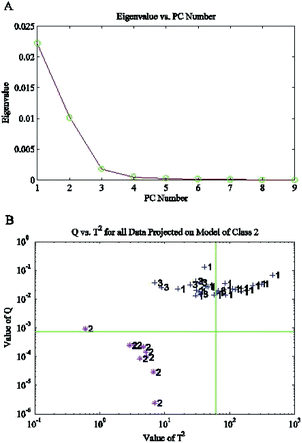
 is formed. The explained percentage of its eigenvalues is shown in Fig. 13. The 2 eigenvectors corresponding to the 2 largest eigenvalues make up the transformation matrix W1(800 × 2). Similarly, from Section 3.3, the within-class scatter matrix Sw is formed to represent the classification features from the class centering eigenvectors. The eigenvectors with the 3 smallest entropies are chosen to form the transformation matrix W2(800 × 3). With the matrices W1(800 × 2) and W2(800 × 3),the extracted classification features t1(39 × 3) and t2(39 × 3) are illustrated in Fig. 14. Obviously, features extracted from the same class will be aggregated, while features extracted from different classes will be separated from each other. The prediction results on the validation set are shown in Table 5. Our proposed method achieves a 100% accurate classification rate. Compared with SIMCA and LS-SVM, it is clear that the proposed method has a higher accuracy.

