Soft-trilinear constraints for improved quantitation in multivariate curve resolution

Abstract

Nowadays, hyphenated chemical analysis methods like GC/MS, LC/MS, or HPLC with UV/Vis diode array detection are widely used. These methods produce a data matrix of mixtures measured during the analytical process. When a set of samples is to be analyzed with one data matrix per sample, the data is often presumed to have “trilinear” structure if the profile for each compound does not change shape or position from one sample to the other. By applying this information as a trilinearity constraint in Self Modeling Curve Resolution (SMCR) methods, overlapping peaks related to the pure compounds of interest can be resolved in a unique way. In practice, many systems have non-trilinear behavior due to deviation from ideal response, for example, a sample matrix effect or changes in instrumental response (e.g., shifts or changes in the shape of chromatographic peaks). In such cases, the trilinear model is not valid because every analyte does not have the same peak shape or position in every sample. In such cases, the unique profiles obtained by strictly enforced trilinearity constraints will not necessarily produce true profiles because the data set does not follow the assumed trilinear behavior. In this work, we introduce “soft-trilinearity constraints” to permit peak profiles of given components to have small deviations in their shape and position in different samples. The advantages and disadvantages of this approach are compared to other methods like PARAFAC2. We illustrate the influence of soft-trilinearity constraints on the accuracy of SMCR results for the case of a 3-component simulated system and an experimental data set. The results show that implementing soft-trilinearity constraints reduces the range of possible solutions considerably compared to the application of constraints such as just non-negativity. In addition, we show that the application of hard-trilinearity constraints can lead to solutions that are completely wrong or exclude the opportunity of a possible solution at all.

---

1. Introduction

The rapid development of analytical instrumentation and data collection tools in recent years has led to the production of multi-way data arrays for a single sample. Experimental measurements generated by analytical instruments are called second-order (i.e., produce three-way data) when there is one matrix per sample (spectra measured over time).¹ Instruments that generate second-order data include hyphenated instruments such as high-performance liquid chromatography coupled with diode array detection (HPLC-DAD), gas chromatography-mass spectrometry (GC-MS) and liquid chromatography-mass spectrometry (LC-MS). Under ideal conditions, the data arrays produced by the above-mentioned instruments have a bilinear structure. A trilinear data structure occurs when several samples are run under identical conditions and have one or more constituents in common. Stacking the individual sample data matrices into a data cube produces a second-order data set. Second-order data sets with trilinear structure have a special property known as the “second-order advantage” that can be exploited to perform quantification of known substances and accurately estimate the concentrations of individual components of interest in the presence of unknown interferences. For these reasons, three-way trilinear data analysis methods, especially second-order calibration, is an active area of research that has been gaining widespread acceptance in a variety of scientific fields, such as chemistry, medicine, food and environmental research.^2–5

A number of different algorithms have already been proposed for the decomposition of three-way data arrays. Some of these methods can be used to decompose a three-way data set, D (m × n × p), based on generalized eigenanalysis such as the generalized rank annihilation method (GRAM),^5,6 and direct trilinear decomposition (DTLD).⁷ There are other decomposition methods for three-way data arrays that are based on iterative procedures, such as parallel factor analysis (PARAFAC)⁸ and the alternating trilinear decomposition method (ATLD).⁹ Additionally, the analysis of three-way data can be conducted as a special case of the bilinear factorization method using Multivariate Curve Resolution (MCR). The MCR method can be applied to three-way data arrays that follow the bilinear model for each sample; however, it is not necessary that they follow trilinearity for the whole data set.¹⁰ MCR,^11,12 is defined as a method to mathematically resolve a measured data matrix of mixtures from hyphenated analytical methods by determining the pure component concentration profiles and the pure component spectral profiles using minimal constraints such as non-negativity. The mathematical solutions of these methods may not be unique because of rotational ambiguity, meaning there is a range of feasible solutions that fulfill the constraints and represent the measured data correctly.¹³ Therefore, consideration of all feasible solutions can provide useful information about the data set under study.^14–21 In order to reduce rotational ambiguity, additional information in the form of constraints can be used. These constraints^21–23 represent additional physical–chemical information about the components in the mixture.

Imposing chemically meaningful constraints can lead to a smaller range of feasible solutions. In the case of the analysis of three-way data sets by MCR, trilinearity constraints can be imposed such that the pure component profile of one or more components remains invariant between the different samples. When ideal trilinear behavior is observed, the collection of resolved profiles of the component of interest from each sample gives a rank-one matrix,¹⁰ such that the components of interest are mathematically resolved in a unique way. In practice, the analysis is complicated by the fact that there are frequently small changes in peak shape and peak position of the components of interest from sample to sample (e.g., peak shifts or width changes in the chromatogram). Moreover, the sensitivity of the spectral response can change in the presence of different chemical matrix effects in the sample (the so-called matrix effect). For these reasons, a strict trilinear model is often not valid, and every component of interest will not have the same concentration profile in every sample. In such cases, the unique profiles obtained by strictly enforced “hard” trilinearity constraints, are not necessarily the true profiles because the data set does not exhibit ideal trilinear behavior. Some algorithms have been introduced to handle such non-trilinear behavior while retaining a mathematically unique solution, such as PARAFAC2.^24–26

“Soft” constraints that allow small deviations from constrained values were introduced by Gemperline.^27,28 He introduced a new algorithm using least squares penalty functions to implement constraints during alternating least squares steps. Later, Rahimdoust et al. visualized the effect of soft constraints on the accuracy of self-modeling curve resolution methods.²⁹ They introduced new, improved cost functions to be used during the MCR optimization process to apply non-negativity, unimodality, equality, and closure constraints and compared the results with those calculated by hard constraints. They demonstrated that imposing “hard” constraints when non-ideal behavior is observed can result in mathematical solutions that lie outside the set of feasible solution boundaries. In such cases, the resulting solution may suffer from active constraints due to non-ideal chemical response. Therefore, based on recent studies, applying soft constraints can produce more reliable results when the properties of the two-way data array are non-ideal.

In this work, we introduce “soft-trilinearity constraints” and a new MATLAB program to permit peak profiles of the components of interest to have small deviations in their shape and position from sample to sample. In order to visualize the results, soft-trilinearity constraints were incorporated into a systematic grid search algorithm for the case of a three-component system.³⁰ This algorithm is general and can be applied to any MCR method. Results are provided for noisy simulated data with non-trilinear behavior and one experimental data set. The results show that implementing soft-trilinearity constraints reduces the range of feasible solutions considerably compared to the application of simpler non-negativity constraints. The results of this approach are compared to other methods, including PARAFAC2 and MCR-ALS, with hard-trilinearity³¹ constraints. It is shown that the methods employing hard-trilinearity constraints lead to incorrect solutions, or produces solutions outside the range of feasible solutions.

2. Theory

Many hyphenated analytical methods (for example, HPLC with VU/Visible diode array detection) produce a bilinear data matrix, D (m × n) of measured responses, where a linear relationship exists between the measured response and the concentrations of the chemical species in a mixture (eqn (1)) where m represents the number of measured spectra (responses) at n wavelengths for nc components.

D_(m×n) = C_(m×nc)A^T_(nc×n) + E_(m×n) (1)

In eqn (1), the matrix C (m × nc) contains the nc concentration profiles in its columns, and the matrix A^T (nc × n) contains the nc pure component spectra of those components in its rows. The error matrix, E, comprises residuals (noise) or non-modeled parts of D, which has the same dimension as D.

A frequent first step in MCR is to perform a decomposition of the data matrix by using the singular value decomposition (SVD) or principal component analysis (PCA):

By use of the SVD or PCA, the bilinear data matrix, D, can be decomposed giving left eigenvectors U (m × nc), right eigenvectors V (nc × n) and a diagonal matrix of singular values S (nc × nc), where the orthonormal U and V matrices define the basis vectors of the column and row spaces, respectively. In eqn (2), the matrix T is a nonsingular transformation matrix that transforms the abstract solutions (US and V^T) into the concentration profiles and pure spectral response profiles, where TT⁻¹ = I and I is an identity matrix. The rows of matrix T and the columns of matrix T⁻¹ represent the coordinates of the feasible solutions in row and column space, respectively. The dimension of the T and T⁻¹ matrices are nc × nc based on the number of components in the system. There are a number of published procedures to estimate the range of feasible solutions for two-component, three-component, and higher component mixtures.^15–21 In this work, a systematic grid search method for three-component systems was modified to include soft-trilinear constraints and used to find the range of possible T_(3×3) matrices that define the correct C and A^T based on eqn (2) and chemically meaningful constraints. In order to perform this task, the standard simplex algorithm for nonlinear optimization (fminsearch in MATLAB) was used. In the case of three-component systems, the T matrix has nine elements, which can be reduced to six elements in normalized form by dividing each row of the T matrix by its first element. For example, for the first component, the values of t₁₂ and t₁₃ are searched in a 2 × 2 grid for a feasible solution (one that obeys all constraints) while the other coefficients in the sub-matrix F are optimized using fminsearch:

During the calculation of C = UST⁻¹ and A^T = TV^T, the physical constraints on the calculated concentration and spectral profiles are tested, and feasible solutions at each grid point can be defined as the set of rotation matrices, T, that give feasible solutions which fulfill the applied constraints.

2.1. Soft-trilinearity constraints

Soft-trilinearity constraints were implemented by defining a constant, α, that determines the degree of softness allowed. The parameter for the evaluation of each component under soft-trilinearity constraints is δ_α. The procedure for imposing soft-trilinearity constraints is as follows where the coefficient, k, is computed at each iteration according to eqn (4), and nf is the number of augmented or folded matrices.

1. For the ith component:

  a. Fold the current estimate of the concentration profile of component i into a matrix

2. Apply PCA to the matrix

3. Calculate the value of k, according to eqn (4).

4. If k ≤ α, then

  δ_α = 0

 else

  r = c_i–c_i-hat

5. δ_α = ∑∑(r × r^T)

 where, c_i-hat=|(u_c (:,2:nf) s_c (2:nf,2:nf) v^T_c (:,2:nf))|

6. end if

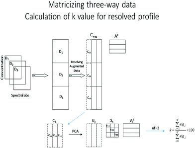
In order to calculate the value of k for the ith component (presented graphically in Scheme 1), the resolved profile with dimension of (m × nf) × 1 for the augmented data set is folded into a new matrix c_i (m × nf), where m is the number of rows in each data matrix and nf is the number of augmented data matrices according to the above procedure. This matrix is decomposed by PCA. If the resolved concentration profiles in the different matrices do not have any deviation from trilinearity, they will have the same shape, and only the first principal component will be significant. In the case of non-ideal chemical behavior, the resolved profiles will differ in shape, so additional principal components will be meaningful. In this procedure, the value of k for imposing soft-trilinearity constraints is the percentage of the summation of all eigenvalues except the first one, divided by the summation of all eigenvalues (eig_j is j'th eigenvalue obtained by using PCA on the folded concentration profiles).

Scheme 1 Implementation of trilinearity soft constraints. The concentration profiles in the first column of the resolved concentration matrix [c₁₁;c₁₂;c₁₃] are folded to give the matrix C₁. By applying PCA to C₁, eigenvalues are obtained, and then k is calculated. This procedure is applicable for any component which is desired to follow trilinearity constraints.

In the case that the estimated profiles fulfill the soft constraint, δ_α is equal to zero and if not, δ_α is greater than zero. By increasing the value of α, larger deviations from ideal trilinearity behavior are allowed, causing the area of feasible solutions (AFS) for the analyte under consideration to be expanded. Adjustment of the parameter α is a crucial step, and the application of soft-trilinearity constraints restricts the range of possible T matrices. The parameter α must be chosen for the system under study such that the amount of expected deviation from ideal trilinear behavior is based on prior information about the reproducibility of the analytical method under consideration. If α is too large, then trilinearity constraints are weakly applied, and in the limit, the AFS borders for the analyte of interest would be the same as borders without trilinearity and just non-negativity constraints. In contrast, if α = 0, hard-trilinearity constraints are imposed, and the profile of the compound in different matrices must be exactly the same.

If the calculated k value for component i is less than α, the grid point is accepted as a location with concentration profiles that obey soft-trilinearity behavior; otherwise, it is not a proper solution, and its deviation from trilinearity is more than the accepted level (see ESI†)

3. Data

3.1 Example 1, simulated data

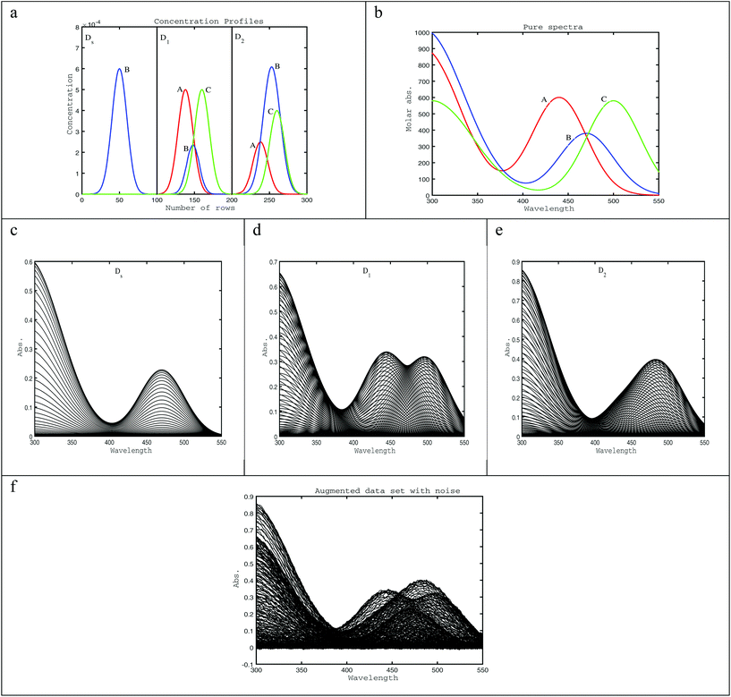
To illustrate the situation where second-order data does not have an ideal trilinear structure, 3 chromatographic based data matrices; D_s, D₁, and D₂ were simulated. D_s is a standard of one component (B), which is the analyte of interest having a retention time of R_s = 50 and a full-width at half-maximum (W_s = 23.55). D₁ and D₂ are samples having mixture data matrices, each containing three components, one being the analyte of interest overlapped with two unknown interference peaks. Non-ideal trilinear behavior of the analyte peak is modeled by deviations in retention time, R_t, and peak width, W. The peak maxima (R_t) of the analyte in D₁, and D₂ is shifted to R_t1 = 48 and R_t2 = 53 respectively, and the peak width of the analyte is changed to W₁ = 20.02 and W₂ = 27.09 in D₁, and D₂ in turn. Plots of the simulated elution profiles are shown in Fig. 1a, and the pure component spectra of three components are shown in Fig. 1b. The simulated elution profiles are Gaussian, while spectra are linear combinations of two Gaussians. The individual data matrices have the same dimensions (Fig. 1c–e) of 100 elution times and 126 wavelengths. The augmented data matrix, D_aug, is built from the individual data matrices, D_s, D₁, and D₂, which are augmented column wise [D_s; D₁; D₂]. The size of this augmented matrix is (3 × 100, 126). Finally, in order to consider the effect of noise that is unavoidable in real data sets, 0.5% of the maximum value of the augmented data is added to D_aug (Fig. 1f).

Fig. 1 (a) Simulated concentration profile(s), (b) simulated spectra profiles, (c) D_s, standard matrix of analyte with R_ts = 50 and W_s = 23.55; (d) D₁, first mixture with R_t1 = 48 and W = 20.02 for analyte and (e) D₂, second mixture data with R_t2 = 53 and W = 27.09 for analyte (f), D_aug, augmented data with added noise amount of 0.5% maximum of the data set.

3.2 Example 2

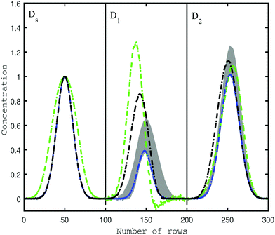
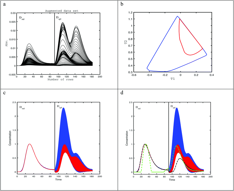
A real experimental case is used to illustrate the proposed algorithm in the quantitative analysis of an HPLC-DAD chromatogram of a three-component system with two identified pesticides (azinphos-ethyl and fenitrothion) and one unknown interferent.^31,32 In this example, only one analyte was of interest, azinphos-ethyl. A three-way data set was formed by column-wise augmentation of one standard data matrix containing only azinphos-ethyl with one sample data matrix of three compounds (both analytes and one unknown interferent). This data set was downloaded from http://www.cid.csic.es/homes/rtaqam/tmp/WEB_MCR/download_dataHPLC.html. Noisy spectra in the first 8 rows of the data matrix were deleted, so the remaining data matrix had dimensions 91 × 73.

4. Results and discussion

In order to evaluate the effect of soft-trilinearity constraints on the area of feasible solutions (AFS), the simulated and experimental data sets described above were analyzed using the new soft-trilinear constraint algorithm described in section 2.1. Both were three-component data sets with non-trilinear behavior. The analysis of the augmented data sets using the systematic grid search method and soft non-negativity constraints for concentration profiles and absorbance profiles produced the range of feasible solutions.

4.1 The AFS under soft non-negativity constraints

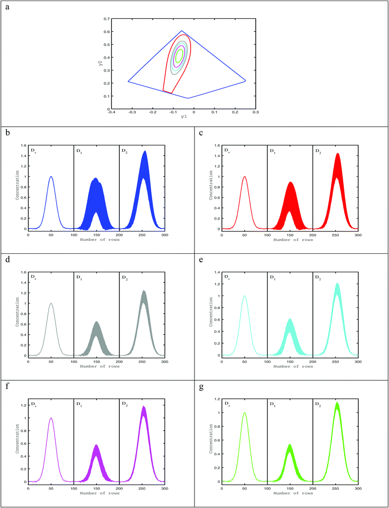
As reported before in the literature,^27–29 by using soft non-negativity constraint, the borders of the area of feasible solutions can be calculated, showing bounded regions with no active constraints. In the case of soft non-negativity constraints, small negative deviations that lie within known noise levels of the data sets are accepted. In order to accept small deviations from non-negativity of the C and A matrices, the noise levels in resolved profiles must be estimated. In this way, a defined threshold for accepting the profiles is 6 times the median absolute deviation (MAD) from a double smoothing procedure. For this purpose, the estimated concentration and spectral profiles are smoothed by a three-point binomial filter. The difference between the smoothed and unsmoothed profiles is calculated as the residual. The median absolute deviation of the difference between smoothed residual and unsmoothed residual is set as the noise level for each resolved profile, 6xMAD.¹⁷Fig. 2a and b represents the AFS and concentration profiles of the analyte of interest (component B) under soft non-negativity constraint.

Fig. 2 (a) Area of Feasible Solutions (AFS) for analyte (component B) where y1 and y2 are the coordinates (scores) of the projected column vectors in the concentration space. Non-negativity and soft trilinearity constraints were used with different alpha levels (see text) [α = 1.60, 1.54, 1.52, 1.51, 1.49] giving corresponding translated concentration profiles in panels (b–g).

4.2. The reduction of AFS under soft-trilinearity constraints

4.2.1. Example 1. In order to study the effect of implementing the new algorithm of section 2.1 on the accuracy of the results obtained by soft-non-negativity constraints, soft-trilinearity constraints for component B were applied. Fig. 2a shows the calculated range of possible solutions obtained by imposing non-negativity and different levels of soft-trilinearity constraints. The blue line in Fig. 2a shows the AFS border using just non-negativity constraints. The corresponding range of concentration profiles for the analyte, compound B, is shown in Fig. 2b. All of the illustrated concentration profiles are normalized to the maximum value of the standard profile. Trilinearity constraints were applied with different levels of α. For α = 1.60, the calculated AFS and translated concentration profiles are shown in red (Fig. 2a and c). Likewise, for α = 1.54, 1.52, 1.51, and 1.49, the borders of calculated AFS's and corresponding concentration profiles are shown in grey, cyan, pink, and green, respectively. It is obvious that with lower α values, the obtained AFS's related to analyte (B) are decreasing in size as well. In other words, at higher levels of α, fewer trilinear profiles are accepted as feasible solutions; thus the selection of a proper level for α influences the accuracy of results. Therefore, to have a reliable analysis, the correct estimation of α is crucial. In Example 1, the lowest accepted value for imposing trilinearity constraint is α = 1.54. As is shown in Fig. 3, the real profile for component B shown as a dashed-dotted blue line falls within the border of the range of possible solutions obtained with α = 1.54. Consequently, with values lower than this amount, the real answer will be out of the calculated range, and the obtained result will not be accurate. Moreover, the calculated quantitative concentration ranges with non-negativity, and trilinearity constraints are summarized in Table 1. As can be seen in Table 1, the actual concentration of component B in D₁ and D₂ is 2.00 × 10⁻⁴ and 7.00 × 10⁻⁴ (AU), respectively. With non-negativity constraints, a range of possible concentration values is obtained (see Table 1). By imposing trilinearity constraints these ranges are decreased. Considering the quantitative results, it is revealed that the minimum possible value for α is 1.54, which leads to a concentration range of 1.90 × 10⁻⁴ to 4.80 × 10⁻⁴ and 6.95 × 10⁻⁴ to 8. 97 × 10⁻⁴ (AU) in D₁ and D₂, respectively. Hence, with lower values of α, the true values of analyte are out of the calculated concentration ranges. In real cases, chemists may know the amount of deviation from ideal trilinear behavior from different changes in retention time and peak width (broadening). For example, in the pharmaceutical industry, by using USP best practices such as system suitability testing and assay reproducibility testing, the range of acceptable values of R_t and W for a particular method can be estimated. This information can be used to reliably adjust the parameter α so that calculated concentration profiles with soft-trilinearity constraints can be achieved. As a best practice, imposing any constraint in SMCR should be based on chemical information, otherwise, the obtained results may be biased. To conclude, in Example 1 it is shown that by decreasing the value of α, the AFS will decrease as well. Depending on how soft of a profile constraint that can be accepted, this parameter can be tuned, but this justification must be based on prior knowledge. If there is no information about the chemical behavior of components, it is better to rely on the range of possible solutions obtained by non-negativity alone rather than imposing other constraints. Moreover, when there is one experiment, including only one standard, the use of equality constraints could be recommended. However, earlier research has shown that the equality constraint, in this case, does not have any effect on the concentration range of the analyte but provides a unique spectrum for this compound and will affect the concentration range of the other components.^33,34

Fig. 3 Range of calculated concentration profiles (grey) with soft trilinearity constraints (α = 1.54), PARAFAC2 result (green) and MCR-ALS result for Example 1 (black). Real profiles are shown for reference (blue).

Table 1 Calculated concentration values associated with the application of soft-trilinear constraints using different levels of α and methods using hard-trilinear constraints, PARAFAC2, and MCR-ALS for analyte (B) in simulated HPLC data set

	Concentration values in D1	Concentration values in D2
True values	2.00 × 10^−4 (AU)	7.00 × 10^−4 (AU)
Soft non-negativity constraint	1.20 × 10^−4–8.34 × 10^−4	6.53 × 10^−4–1.10 × 10^−3
Soft-trilinear constraint α = 1.60	1.45 × 10^−4–7.46 × 10^−4	6.67 × 10^−4–1.10 × 10^−3
Soft-trilinear constraint α = 1.54	1.86 × 10^−4–4.80 × 10^−4	6.95 × 10^−4–8.97 × 10^−4
Soft-trilinear constraint α = 1.52	1.99 × 10^−4–4.40 × 10^−4	7.03 × 10^−4–8.70 × 10^−4
Soft-trilinear constraint α = 1.51	2.18 × 10^−4–4.03 × 10^−4	7.16 × 10^−4–8.43 × 10^−4
Soft-trilinear constraint α = 1.49	2.45 × 10^−4–3.59 × 10^−4	7.34 × 10^−4–8.13 × 10^−4
MCR-ALS	5.44 × 10^−4	8.70 × 10^−4
PARAFAC2	4.66 × 10^−4	5.78 × 10^−4

---

4.3. Hard constraints

4.3.1. Example 1. As mentioned before, some algorithms have been developed to deal with non-trilinear data sets. A well-known method for resolving an augmented data set is multivariate curve resolution–alternating least squares (MCR-ALS), which works by forcing trilinear structure on the profiles in the augmented mode. When the data is non-trilinear, as is shown, examining the results obtained by MCR-ALS with non-negativity constraints and hard-trilinearity constraints (just for the analyte) shows the danger of applying unsuitable constraints to a data without knowing first if it is really trilinear (see Fig. 3, black dashed-dotted line). Moreover, the obtained result for quantitative analysis can be biased as well. Table 1 shows that concentration values for component B with hard constraints are 5.44 × 10⁻⁴ and 8.70 × 10⁻⁴ in D₁ and D₂ respectively, while the true values are 2.00 × 10⁻⁴ and 7.00 × 10⁻⁴, respectively. Another well-known method for analyzing non-trilinear data sets is PARAFAC2, which is known to always converge to a unique solution. PARAFAC2 allows a certain freedom in the shape of the profiles in the variable mode. To keep uniqueness in the solutions, all cross-product matrices X_kX^T_k are forced to be constant over k, i.e., X₁X^T₁ = X₂X^T₂ = ⋯ = X_kX^T_k, where matrix X is the mode with variation in the shapes of profiles. This condition is fulfilled in particular situations, for example, in chromatographic data sets where the concentration profiles are shifted by the same amount between pairs of X_k matrices, but there are no changes in the shapes of the profiles of each component. This condition is not suitable for all non-trilinear data sets, especially when there are changes in peak widths. Therefore, as is shown in Fig. 3 (green dashed-dotted line), the PARAFAC2 method with non-negativity constraints gives a solution that it is not physically correct. The peak profiles obtained are far from the feasible solutions (shaded grey bands). These results indicate that in this example there is no profile that fulfills the condition of invariance in the X_kX^T_k product over all three data sets in the augmented matrix; therefore the quantitative results with obtained by PARAFAC2 are inaccurate. Table 1 shows that concentration values for component B with PARAFAC2 are 4.97 × 10⁻⁴ and 5.78 × 10⁻⁴ in D₁ and D₂, respectively. It is thus shown that imposing an unreliable constraint, that is forcing the resolved profiles to have exactly the same shape, can lead to a unique solution that is wrong, affecting the quantitative accuracy of the resolved profiles. In situations similar to this example where non-trilinear behavior is observed, the results obtained from soft-trilinear constraints are likely to be more reliable than those that are calculated under hard constraints.

4.3.2 Example 2. In this example, a mixture of three components consisting of azinphos-ethyl and fenitrothion with an unknown interferent is analyzed, where azinphos-ethyl is analyte of interest. The column-wise augmented data consists of a standard and mixture data set (Fig. 4a). The blue line in Fig. 4b shows the calculated AFS with non-negativity constraints. The corresponding concentration profiles are shown in Fig. 4c in blue, as well. All of the illustrated concentration profiles are normalized to the maximum value of the standard profile. Using α = 3 and soft-trilinearity constraints lead to a range of possible solutions that are shown in red (Fig. 4b and c). As before, the quantitative values for the relative concentration of azinphos-ethyl under non-negativity and trilinearity constraints are calculated and summarized in Table 2 (the concentration of the analyte in the standard sample is assumed to be 1 AU). Also, the results obtained with MCR-ALS by imposing non-negativity and hard-trilinearity constraints and PARAFAC2 with non-negativity constraints are depicted in Fig. 4d with black and green dashed lines, respectively. Also, the non-negativity constraint is applied to the resolved concentration profile by PARAFAC2 due to negative values. As was seen in Example 2, the solutions provided by MCR-ALS and PARAFAC2 do not fall within the range of feasible solutions. Therefore, using these profiles for quantitative analysis gives poor results (Table 2).

Fig. 4 (a) Data set of Example 2, (b) calculated AFS for azinphos-ethyl with soft nonnegativity (blue) and soft trilinearity constraint (red), (c) translated concentration profiles, (d) result of PARAFAC2 (green) and MCR-ALS (black).

Table 2 Calculated concentration values associated with the application of soft-trilinear constraint using α = 3 and methods using hard-trilinear constraints, PARAFAC2, and MCR-ALS for azinphos-ethyl in experimental HPLC data set

	Relative concentration values (AU)
Soft non-negativity constraint	0.54–2.07
Soft-trilinear constraint using α = 3	0.57–1.19
MCR-ALS	0.49
PARAFAC2	1.57

---

4.4. RSM

An experimental design was created using the two simulated data sets in Example 1 to study the main effects and interaction of retention time, peak width, and noise level on the accuracy of concentration profiles produced by soft-trilinear constraints. A three-factor, two-level central composite experimental design was used, where the controlled factors were retention time of the analyte (X), peak width of the analyte (Y), and the measurement noise level (Z). Two matrices D_s and D₁ were augmented, the first being the standard matrix containing one component, the analyte of interest, and the second being a mixture of the three components shown in Fig. 1c and d. In order to simulate a non-trilinear data set, the retention times and peak widths of the concentration profile of the analyte in the second data matrix were perturbed by known amounts as dictated by the experimental design. The three controlled factors, retention time (X), peak width (Y), and noise level of the augmented data (Z), were adjusted based on the levels listed in Table 3. By changing these three factors, 15 data sets were generated. After applying soft-trilinearity constraints, the AFS for the concentration profile of the analyte was calculated. The resulting band of transformed concentration profiles was used to calculate the area difference between the upper and lower band for use as the response variable of the experimental design. The responses were fitted to the factors via multiple regression using Quantum XL program downloaded from http://www.sigmazone.com/QuantumXLdownload.htm. The response surface plot (Fig. 5) shows that in this example, the peak-broadening effect has the largest influence on deviation from trilinearity. eqn (1) shows the contributions of individual factors and interactions between factors on the accuracy of results. Looking at the main effects, the regression coefficient for factor Y (peak-broadening) confirms that Y has the most significant influence on the response, while factor X (retention time shifts) has the smallest influence on the response. Also, it is clear that XZ (interaction of retention time and noise) has the biggest influence among the interaction of factors. Note that this result is valid for this particular simulated data set and may not be the same for all cases with different non-ideal situations.

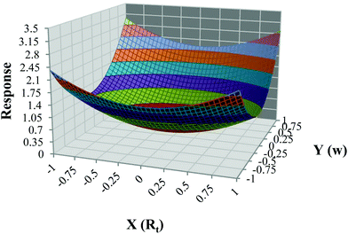Fig. 5 Obtained Response Surface for different non-trilinear behaviors due to changes in retention time (X), peak width (Y) and noise level.

Table 3 Three-level fractional factorial design

Factor	Range		Setpoint
	Low	High
X	−1 (48)	1 (53)	0 (50)
Y	−1 (8.5)	1 (11.5)	0 (10)
Z	−1 (0.1% max data)	1 (1% max data)	0 (0.5% max data)

---

5. Conclusion

Using reliable constraints to narrow the range of possible solutions is an interesting subject in SMCR methods. Some of these constraints are more robust and lead to unique solutions. In this work, trilinearity constraints were studied, which many SMCR methods apply as a hard constraint. By implementing hard constraints and forcing the resolved profiles of all matrices to have the same shape or follow special patterns of variation can lead to incorrect solutions, and it can be expected that many real-world data sets suffer from these kinds of shifts and small changes in the shape of profiles. In this work, we introduced soft-trilinearity constraints and showed its advantages in simulated and experimental data sets. This approach is generally useful in many circumstances and leads to solutions that are more accurate than those that are obtained with hard constraints. Moreover, the use of soft constraints allows for the possibility to tune the AFS boundary based on chemical information about the sample and method reproducibility.

Conflicts of interest

There are no conflicts to declare.

References

1. E. Sanchez and B. Kowalski, J. Chemom., 1988, 2, 247–263.
2. K. S. Booksh and B. R. Kowalski, Anal. Chem., 1994, 66, 782A–791A.
3. V. Gómez and M. P. Callao, Anal. Chim. Acta, 2008, 627, 169–183.
4. H.-L. Wu, J.-F. Nie, Y.-J. Yu and R.-Q. Yu, Anal. Chim. Acta, 2009, 650, 131–142.
5. E. Sanchez and B. R. Kowalski, Anal. Chem., 1986, 58, 496–499.
6. B. E. Wilson, E. Sanchez and B. R. Kowalski, J. Chemom., 1989, 3, 493–498.
7. E. Sanchez and B. R. Kowalski, J. Chemom., 1990, 4, 29–45.
8. R. Bro, Chemom. Intell. Lab. Syst., 1997, 38, 149–171.
9. H. L. Wu, M. Shibukawa and K. Oguma, J. Chemom., 1998, 12, 1–26.
10. R. Tauler, I. Marqués and E. Casassas, J. Chemom., 1998, 12, 55–75.
11. W. H. Lawton and E. A. Sylvestre, Technometrics, 1971, 13, 617–633.
12. R. Tauler, B. Kowalski and S. Fleming, Anal. Chem., 1993, 65, 2040–2047.
13. H. Abdollahi and R. Tauler, Chemom. Intell. Lab. Syst., 2011, 108, 100–111.
14. O. S. Borgen and B. R. Kowalski, Anal. Chim. Acta, 1985, 174, 1–26.
15. P. D. Wentzell, J.-H. Wang, L. F. Loucks and K. M. Miller, Can. J. Chem., 1998, 76, 1144–1155.
16. R. Rajkó and K. István, J. Chemom., 2005, 19, 448–463.
17. P. J. Gemperline, Anal. Chem., 1999, 71, 5398–5404.
18. M. Sawall and K. Neymeyr, J. Chemom., 2014, 28, 633–644.
19. A. Golshan, H. Abdollahi, S. Beyramysoltan, M. Maeder, K. Neymeyr, R. Rajkó, M. Sawall and R. Tauler, Anal. Chim. Acta, 2016, 911, 1–13.
20. R. Tauler, J. Chemom., 2001, 15, 627–646.
21. A. Golshan, H. Abdollahi and M. Maeder, Anal. Chim. Acta, 2012, 709, 32–40.
22. M. Sawall, C. Fischer, D. Heller and K. Neymeyr, J. Chemom., 2012, 26, 526–537.
23. S. Beyramysoltan, H. Abdollahi and R. Rajkó, Anal. Chim. Acta, 2014, 827, 1–14.
24. H. A. Kiers, J. M. ten Berge and R. Bro, J. Chemom., 1999, 13, 275–294.
25. R. Bro, C. A. Andersson and H. A. Kiers, J. Chemom., 1999, 13, 295–309.
26. S. A. Bortolato and A. C. Olivieri, Anal. Chim. Acta, 2014, 842, 11–19.
27. P. J. Gemperline and E. Cash, Anal. Chem., 2003, 75, 4236–4243.
28. S. Richards, R. Miller and P. Gemperline, Appl. Spectrosc., 2008, 62, 197–206.
29. N. Rahimdoust Mojdehi, M. Sawall, K. Neymeyr and H. Abdollahi, J. Chemom., 2016, 30, 252–267.
30. A. Golshan, H. Abdollahi and M. Maeder, Anal. Chem., 2011, 83, 836–841.
31. A. De Juan and R. Tauler, J. Chemom., 2001, 15, 749–771.
32. R. Tauler, S. Lacorte and D. Barcelo, J. Chromatogr., A, 1996, 730, 177–183.
33. S. Beyramysoltan, R. Rajkó and H. Abdollahi, Anal. Chim. Acta, 2013, 791, 25–35.
34. G. Ahmadi and H. Abdollahi, Current Applications of Chemometrics, 2015, p. 57.

---

Footnote

† Electronic supplementary information (ESI) available. See DOI: 10.1039/c8an00615f

---