
Theoretical discovery of Dirac half metal in experimentally synthesized two dimensional metal semiquinoid frameworks†
Cheng
Tang
 a,
Chunmei
Zhang
a,
Zhenyi
Jiang
b,
Ken
Ostrikov
a and
Aijun
Du
*a
a,
Chunmei
Zhang
a,
Zhenyi
Jiang
b,
Ken
Ostrikov
a and
Aijun
Du
*a
aSchool of Chemistry, Physics and Mechanical Engineering, Queensland University of Technology, Gardens Point Campus, Brisbane, Queensland 4001, Australia. E-mail: aijun.du@qut.edu.au
bShaanxi Key Laboratory for Theoretical Physics Frontiers, Institute of Modern Physics, Northwest University, Xi’an 710069, P. R. China
First published on 11th April 2019
Abstract
The discovery of half-metallic Dirac cones in metal–organic frameworks (MOFs) opens up new prospects for future spintronic devices. Although this unique feature has been demonstrated in several theoretically designed MOFs, none of these have been synthesized. Therefore, the exploration of half-metallic Dirac features in experimentally synthesized MOFs is extremely significant. In this study, via density functional theory, we investigate two recently synthesized two-dimensional (2D) metal-semiquinoid frameworks (V-SF and Ti-SF) as novel Dirac materials with ultrahigh Fermi velocities (up to 3.74 × 10⁵ m s−1), which are comparable to that of graphene. Notably, Ti-SF exhibits a Dirac dispersion in only one spin channel, while it is semiconducting with a bandgap of 1.67 eV in the other spin channel. This is the first report of a half-metallic Dirac feature in experimentally synthesized MOFs. Furthermore, we adopted a molecular orbital model to analyse the magnetism of MOFs with D3 symmetry. The model accurately describes the magnetism of 3d transition metal-semiquinoid frameworks, and we expected it to instruct further research focused on magnetic complexes.
Introduction
Dirac dispersion was first discovered in graphene and has been theoretically proved in various two-dimensional (2D)1–8 and several bulk materials.9–16 In general, materials with Dirac cones lead to variety novel properties, including half-integral, fractional and fractal Quantum Hall Effects (QHE), ballistic charge transport, and ultrahigh carrier mobility, which primarily meet the requirements of electronic devices.17–19 On the other hand, spintronics materials with 100% spin polarization open up new perspectives for applications in quantum information storage, transportation and processing through combining charges with spins.20–26 Therefore, the combination of massless Dirac fermions and spin-polarized current provides the answer for future high-performance electronic devices. However, up to now, this novel electronic structure is only theoretically predicted to occur in rare 2D structures, including honeycomb and triangular ferrimagnets.27–30In recent years, metal organic frameworks (MOFs) have attracted much attention, due to their wide range of applications in clean energy, storage media, and catalysis.31,32 The large metal–metal separations and the exchange interaction between the metal and organic ligands endow MOFs with adjustable electronic and magnetic properties.33 Hence, MOFs are expected to be ideal candidates for half-metallic Dirac materials. The Quantum Anomalous Hall Effect (QAHE) was first predicted in a 2D triphenyl-manganese (TMn) model in 2013, and its physical origin is attributed to both the intrinsic spin-orbital coupling (SOC) and strong magnetization provided by the Mn atoms.28 Since then, several MOFs with Dirac or other massless fermions have been explored through theoretical methods.34–37 However, most of the predicted Dirac cone MOFs are designed at the molecular level and difficult to synthesize. It is conceivable that the discovery of Dirac half-metallicity in already experimentally synthesized MOFs will greatly promote the progress of fundamental and technical research. Therefore, the exploration of half-metallic Dirac materials among experimentally feasible MOFs is both necessary and significant.
Recently, Ie-Rand et al. were the first to synthesize a 2D iron-semiquinoid framework with a large surface area, indicating its potential for applications in N2 adsorption.38 Subsequently, on the basis of previous study, the metal-semiquinoid frameworks (H2NMe2)2M2(Cl2dhbq)3 (M = Ti and V) and (H2NMe2)2Cr2(dhbq)3 (dhbqn− = deprotonated 2,5-dihydroxybenzoquinone) were fabricated by Micheal and exhibited controllable magnetic and electronic properties.39 However, the lack of theoretical studies on such MOFs hinders a better understanding of their properties and limits their applications. In this study, we present the theoretical frameworks for Dirac cones in two metal-semiquinoid frameworks (V-SF and Ti-SF) through first-principles calculations. Significantly, the Ti-SF shows Dirac cones in one spin channel, while it is semiconducting in the other spin channel, demonstrating its promising applications in spintronics. The estimated Curie temperature of Ti-SF is about 107 K, which is much higher than that of CrI3. Furthermore, we adopted a graphene-type tight-binding (TB) model to reveal the origin of the Dirac cones. The well-fitted band structures near the Dirac points verify the strong π–d conjugation at the valence and conduction bands. Finally, we introduced a molecular orbital model to analyse the magnetism of metal-semiquinoid frameworks (M-SF). Our model not only explains the magnetism of the M-SF we calculated but also successfully predicts the magnetism of all 3d transition metal-semiquinoid frameworks. Thus, this work is expected to instruct future research focused on the development of magnetic complexes with D3 symmetric structures.
Computational details
All the calculations were performed within the framework of density functional theory40,41 (DFT) with the Perdew–Burke–Ernzerhof (PBE) of the generalized gradient approximation42 (GGA), as implemented in Vienna Ab Initio Simulation Package43,44 (VASP). The interaction of the ions and electrons was described by the projector augmented-wave (PAW) method.45 For electronic calculations, we employed the GGA+U46 method and a state-of-the-art Heyd–Scuseria–Ernzerhof47 (HSE) functional to get more accurate results. The kinetic energy cut-off was set to 400 eV, and the vacuum layer set to no less than 15 Å to avoid interaction between the adjacent layers. The K-mesh was set to Gamma-centred 7 × 7 × 1 in first Brillouin Zone (BZ) for the 2D M-SF. The structures were fully optimized until the force and maximum energy of the atoms in each material were no more than 0.001 eV Å−1 and 10−6 eV, respectively. The spin polarizations were also considered in our calculations.Results and discussion
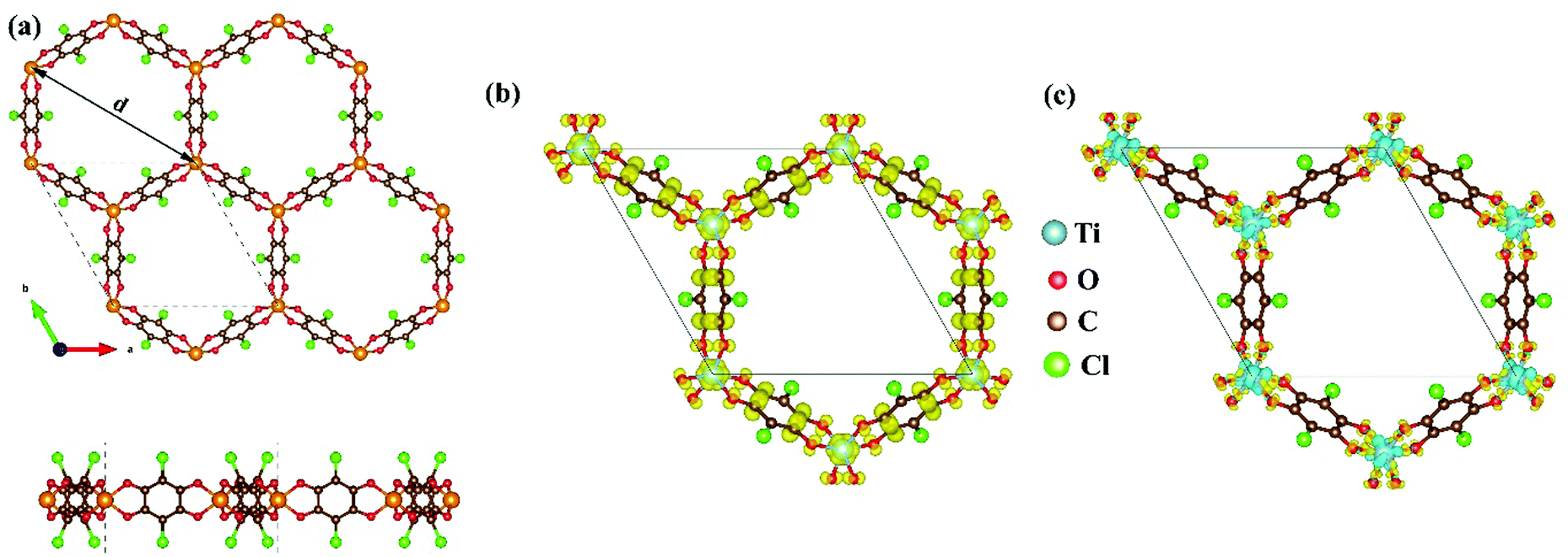
As mentioned above, although the ligand of Cr-SF (dhbq) is different from that of the other M-SFs (Cl2dhbq), simply, we considered that all the M-SFs were compounded with the same ligand (Cl2dhbq). Our electronic property calculations show that the electrons of the chlorine (Cl) atoms will have little impact on the band structure near the Fermi level. The space group of the M-SFs is P![[3 with combining macron]](https://www.rsc.org/images/entities/char_0033_0304.gif) 1m, and the periodic structure is shown in Fig. 1(a). The metal atoms are bridged by three semiquinoid linkers, located in the center of the oxygen octahedron. In order to obtain the magnetic ground state of M-SF, we carefully calculated their energies under different magnetic states (ferromagnetic (FM), antiferromagnetic (AFM), and nonferromagnetic (NM)) (Table S1, ESI†). Only V-SF shows spin quenching, which is consistent with previous experiments.39 The magnetic ground states of Ti-SF and Fe-SF are FM, whereas that of Cr-SF is AFM. For Ti-SF (Fig. 1(b)), the total magnetic moment is 2 μB per unit cell, and the spin states of the semiquinoid linkers are induced by neighboring Ti atoms, resulting in ferromagnetic coupling with between the linkers and Ti atoms.48 By contrast, the spin states are localized on the metal atoms in Fe-SF and Cr-SF (Fig. S1, ESI†).
1m, and the periodic structure is shown in Fig. 1(a). The metal atoms are bridged by three semiquinoid linkers, located in the center of the oxygen octahedron. In order to obtain the magnetic ground state of M-SF, we carefully calculated their energies under different magnetic states (ferromagnetic (FM), antiferromagnetic (AFM), and nonferromagnetic (NM)) (Table S1, ESI†). Only V-SF shows spin quenching, which is consistent with previous experiments.39 The magnetic ground states of Ti-SF and Fe-SF are FM, whereas that of Cr-SF is AFM. For Ti-SF (Fig. 1(b)), the total magnetic moment is 2 μB per unit cell, and the spin states of the semiquinoid linkers are induced by neighboring Ti atoms, resulting in ferromagnetic coupling with between the linkers and Ti atoms.48 By contrast, the spin states are localized on the metal atoms in Fe-SF and Cr-SF (Fig. S1, ESI†).
 | ||
| Fig. 1 (a) Top view and side view of M-SF (M = V, Ti, Cr, Fe). (b) Spin density of the partial Ti-SF structure with an isovalue of 0.005 e Å−3. (c) Charge density difference for Ti-SF with respect to the Ti atoms and ligands. The orange, red, brown, green, and cyan spheres are transition metal, oxygen, carbon, chlorine, and titanium atoms, respectively. The yellow and cyan regions in (c) represent the electron accumulation and depletion areas with an isovalue of 0.02 e Å−3. | ||
The optimized lattice constants, the neighboring metal distances (dM–M), and the aperture diameters (d) of the M-SFs under a magnetic ground state are listed in Table 1. The parameters in our calculation are slightly smaller than those obtained in X-ray diffraction experiment, but the differences are in a reasonable range. The thermodynamical stabilities of M-SF are examined by AIMD calculations at 300 K (Fig. S2, ESI†). The potential energies of the Ti-SF and V-SF fluctuate over a small range during the simulation, while the structures show no significant distortion throughout the process, indicating good thermal stabilities at room temperature. In order to gain insight into the features of charge transfer in M-SFs, we analysed the charge density difference between the metal center and the ligands (see Fig. 1(c) for Ti-SF and Fig. S3, ESI†). For instance, electrons accumulate along the Ti–O bonds and around the O atoms in Ti-SF, indicating electron transfer from Ti atoms to ligands. According to the Bader charge analysis (Table S2, ESI†), there are 1.90, 2.14, 1.81, and 1.55 |e| electrons transferred from the Ti, V, Cr, and Fe atoms to the ligands, respectively. Herein, compared with that in Ti, Cr and Fe cases, the central metal atoms transfer more valence electrons to ligands in V-SF, suggesting a more delocalized electronic structure.39
| a (Å) | d M–M (Å) | d (Å) | |
|---|---|---|---|
| Ti-SF | 13.49 | 7.79 | 15.58 |
| V-SF | 13.29 | 7.67 | 15.34 |
| Cr-SF | 13.18 | 7.61 | 15.21 |
| Fe-SF | 12.96 | 7.49 | 14.96 |
| Experiment datas38,39 | 13.39–13.49 | 7.73–7.84 | 15.66 in Fe-SF |
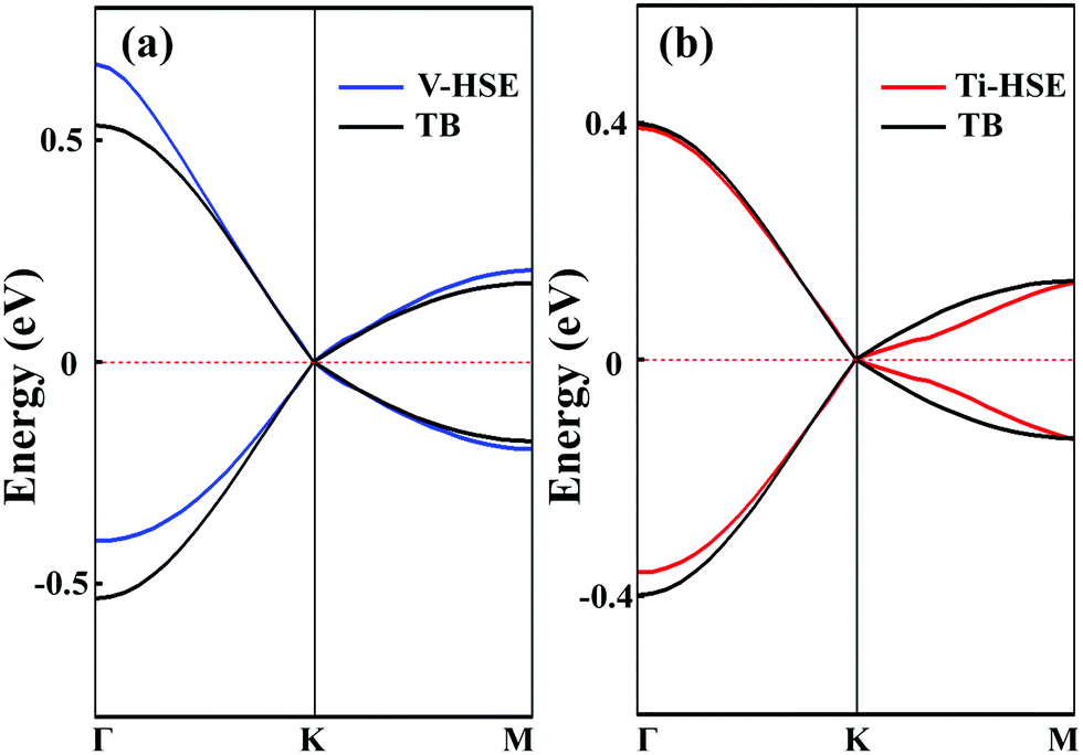
To analyse the electronic properties, the band structures of M-SF were calculated, and the results obtained by GGA_PBE functional are shown in Fig. S4 (ESI†). The Dirac dispersions exist in the band structures of V-SF and Ti-SF. Particularly, Ti-SF shows a Dirac point in one spin channel and a bandgap of 0.69 eV in another spin channel. Therefore, we mainly focused on these two M-SFs with Dirac band dispersion. Fig. S5 (ESI†) displays the density of states for both V-SF and Ti-SF. We can see that the Dirac points are mainly contributed by metal (Ti or V) 3d, oxygen 2p, and carbon 2p orbitals in both two nanosheets. In order to obtain more accurate results, GGA+U (Fig. S6, ESI†) and HSE functionals (Fig. 2) were adopted in the band calculations of V-SF and Ti-SF. The results also demonstrate that the Dirac points (the Dirac cones in 3D band structures) appear at the corners of the BZ in both the valence and conduction bands (K points) of the V-SF and Ti-SF spin up channel, while in spin down channel of Ti-SF, the bandgap expends to 1.67 eV (HSE result). The Fermi velocity (Vf) can be defined as  , where ħ represents reduced Planck constant, and ∂E/∂K is the fitted slopes of the bands at the Dirac point. Thus, the estimated Fermi velocities of V-SF and Ti-SF are 3.74 × 10⁵ and 2.79 × 10⁵ m s−1, respectively, which are comparable to the value of graphene (8.2 × 10⁵ m s−1).3 Then, we analysed the decomposed charge density of M-SF nearby Fermi levels (Fig. 2(b) and (d)). The interaction between the p orbitals of the ligands and the d orbitals of the central metals results in a strong π–d conjugation near the Fermi level, leading to a graphene-type band alignment.36 In addition, V-SF and Ti-SF both have poor mechanical properties, with critical breaking points located at 10% for V-SF and 8% for Ti-SF with respect to the biaxial strain (details in the ESI†).
 | ||
| Fig. 2 Band structures of (a) V-SF and (c) Ti-SF obtained by HSE functional. The insert graphs show the 3D band structures of the Dirac cones within the green circles. The decomposed band charge density near the Fermi levels of (b) V-SF and (d) Ti-SF with an isovalue of 0.004 e Å−3. The Fermi level (red dashed line) has been set to zero. | ||
In order to verify the transition temperature of the material transforming from a FM to an AFM order, the Curie temperature (Tc) is estimated through the mean-field approximation49 (MFA) in combination with the DFT calculation and Heisenberg model. Considering the exchange coupling parameter (J) between the nearest neighbouring magnetic sites, the Curie temperature is expressed as 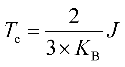 , where KB is the Boltzmann constant and J can be obtained from the energy difference between the AFM and FM order (details in the ESI†). Thus, the calculated Curie temperature of Ti-SF is about 107 K, which is much higher than the calculated Tc of the famous ferromagnetic monolayer CrI3.50
Preceding calculations show a strong π–d conjugation near the Fermi level, leading to a graphene-type band alignment. Therefore, we treated the central metals as the vertexes of a honeycomb sublattice, much like the carbon atoms of graphene (see Fig. S9, ESI†). Thus, the TB Hamiltonian of M-SF can be simply written as
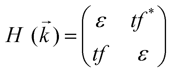
where a is the lattice constant, and Δ is the band gap of K point (0 in both V-SF and Ti-SF), σ represents the Pauli matrix for sublattice, and q = k − K is the momentum vector. Additionally, t′ is the hopping parameter between the nearest neighboring part. To simplify the analysis, we only considered one valley center, the one with
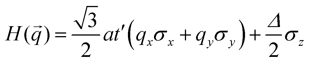
 . As shown in Fig. S10 (ESI†), the bands obtained from the k·p-like model fit well with the HSE results near the Fermi levels. The fitted hopping parameters are 0.041 and 0.025 for V-SF and Ti-SF, indicating the stronger neighboring interaction in V-SF, which is the same as the tight-binding results.
 | ||
| Fig. 3 Band structures of (a) V-SF and (b) Ti-SF calculated by the HSE and TB methods. | ||
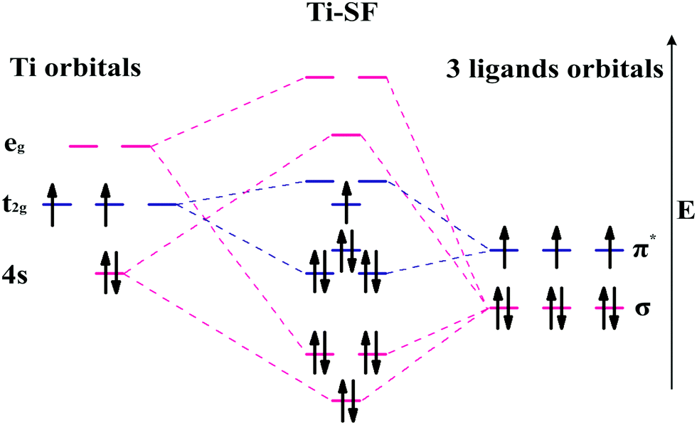 | ||
| Fig. 4 Schematic of molecular orbital model of Ti-SF with local D3 symmetry at the metal center. | ||
Based on the linear combination of atomic orbitals (LCAO), molecular orbital theory provides an efficient approach to predict the magnetism of molecules. However, this theory is still difficult to perform on the complexes containing polyatomic ligands due to the complicated atomic orbitals. Although, the π–π* interactions between metals and ligands are considered as to be the origin of electron delocalization observed for these M-SFs in pioneering research,39 it can not explain the changes in magnetism. Herein, by considering both the σ–σ and π–π interactions between the ligands and metals (Fig. 4), we successfully analysed the magnetism of M-SF. In our model, one unpaired electron exists in the molecular orbitals of Ti-SF, indicating its magnetic state. For V-SF (shown in Fig. S11, ESI†), all the electrons are paired in the molecular orbitals; thus, V-SF is nonmagnetic. Then, we also examined the magnetic properties of Fe-SF and Cr-SF and found the results to be consistent with the DFT calculations. Furthermore, this model can be extended to predict the magnetism of other unsynthesized complexes with D3 symmetry (Sc-SF, Co-SF, and Cu-SF are all nonmagnetic), therefore instructing future research focused on the development of magnetic complexes (details in the ESI†).
Conclusions
In summary, through first-principles calculations we demonstrated that Dirac cones exist in two recently synthesized 2D metal-semiquinoid frameworks (V-SF and Ti-SF) with high Fermi velocities (3.74 × 10⁵ and 2.79 × 10⁵ m s−1). A half-metallic Dirac dispersion is predicted for the first time in an already experimentally synthesized 2D MOF. Our graphene-type tight-binding model aligns with the HSE results near the Fermi level, due to the strong π–d conjugation between the central metals and ligands. Finally, we introduced a molecular orbital model to analyse the magnetism of M-SF; this model has successfully predicted several unsynthesized nonmagnetic M-SFs, including Sc-SF, Co-SF, and Cu-SF. The model was also used to identify the magnetism of other complexes with D3 symmetry. Overall, by using the first-principles method, we theoretically report, for the first time, the existence of Dirac half metal in the recently synthesised 2D Ti-SF, suggesting a wide application for the material in spintronic devices.Conflicts of interest
There are no conflicts to declare.Acknowledgements
The authors acknowledge generous grants of high-performance computer resources provided by the NCI National Facility and The Pawsey Supercomputing Centre through the National Computational Merit Allocation Scheme supported by the Australian Government and the Government of Western Australia. A. D. greatly appreciates the financial support by Australian Research Council under Discovery Project (DP170103598). Z. J. also greatly thanks the support by National Natural Science Foundation of China under Grants (No. 51572219, 51872227).References
- S. Cahangirov, M. Topsakal, E. Aktürk, H. Şahin and S. Ciraci, Phys. Rev. Lett., 2009, 102, 236804 CrossRef CAS PubMed.
- A. C. Neto, F. Guinea, N. M. Peres, K. S. Novoselov and A. K. Geim, Rev. Mod. Phys., 2009, 81, 109 CrossRef.
- D. Malko, C. Neiss, F. Vines and A. Görling, Phys. Rev. Lett., 2012, 108, 086804 CrossRef PubMed.
- J. Wang, S. Deng, Z. Liu and Z. Liu, Natl. Sci. Rev., 2015, 2, 22–39 CrossRef CAS.
- Z. Wang, X.-F. Zhou, X. Zhang, Q. Zhu, H. Dong, M. Zhao and A. R. Oganov, Nano Lett., 2015, 15, 6182–6186 CrossRef CAS PubMed.
- Y. Jiao, F. Ma, J. Bell, A. Bilic and A. Du, Angew. Chem., 2016, 128, 10448–10451 CrossRef.
- F. Ma, Y. Jiao, G. Gao, Y. Gu, A. Bilic, Z. Chen and A. Du, Nano Lett., 2016, 16, 3022–3028 CrossRef CAS PubMed.
- A. Du, S. Sanvito and S. C. Smith, Phys. Rev. Lett., 2012, 108, 197207 CrossRef PubMed.
- Q. Gibson, L. Schoop, L. Muechler, L. Xie, M. Hirschberger, N. Ong, R. Car and R. Cava, Phys. Rev. B: Condens. Matter Mater. Phys., 2015, 91, 205128 CrossRef.
- Z. Wang, H. Weng, Q. Wu, X. Dai and Z. Fang, Phys. Rev. B: Condens. Matter Mater. Phys., 2013, 88, 125427 CrossRef.
- Y. Jiao, F. Ma, C. Zhang, J. Bell, S. Sanvito and A. Du, Phys. Rev. Lett., 2017, 119, 016403 CrossRef PubMed.
- Y. Kim, B. J. Wieder, C. Kane and A. M. Rappe, Phys. Rev. Lett., 2015, 115, 036806 CrossRef PubMed.
- R. Li, H. Ma, X. Cheng, S. Wang, D. Li, Z. Zhang, Y. Li and X.-Q. Chen, Phys. Rev. Lett., 2016, 117, 096401 CrossRef PubMed.
- S. M. Young, S. Zaheer, J. C. Teo, C. L. Kane, E. J. Mele and A. M. Rappe, Phys. Rev. Lett., 2012, 108, 140405 CrossRef CAS PubMed.
- F. Ma, Y. Jiao, Z. Jiang and A. Du, ACS Appl. Mater. Interfaces, 2018, 10, 36088–36093 CrossRef CAS PubMed.
- C. Zhang, Y. Jiao, L. Kou, T. Liao and A. Du, J. Mater. Chem. C, 2018, 6, 6132–6137 RSC.
- N. O. Weiss, H. Zhou, L. Liao, Y. Liu, S. Jiang, Y. Huang and X. Duan, Adv. Mater., 2012, 24, 5776 CrossRef.
- C. R. Dean, L. Wang, P. Maher, C. Forsythe, F. Ghahari, Y. Gao, J. Katoch, M. Ishigami, P. Moon and M. Koshino, Nature, 2013, 497, 598 CrossRef CAS PubMed.
- X. Du, I. Skachko, F. Duerr, A. Luican and E. Y. Andrei, Nature, 2009, 462, 192 CrossRef CAS PubMed.
- A. Fert, Rev. Mod. Phys., 2008, 80, 1517 CrossRef CAS.
- S. Wolf, D. Awschalom, R. Buhrman, J. Daughton, S. Von Molnar, M. Roukes, A. Y. Chtchelkanova and D. Treger, Science, 2001, 294, 1488–1495 CrossRef CAS PubMed.
- D. D. Awschalom and M. E. Flatté, Nat. Phys., 2007, 3, 153 Search PubMed.
- C. Felser, G. H. Fecher and B. Balke, Angew. Chem., Int. Ed., 2007, 46, 668–699 CrossRef CAS PubMed.
- C. Huang, Y. Du, H. Wu, H. Xiang, K. Deng and E. Kan, Phys. Rev. Lett., 2018, 120, 147601 CrossRef PubMed.
- X. Wang, Phys. Rev. Lett., 2008, 100, 156404 CrossRef CAS PubMed.
- X.-L. Wang, Natl. Sci. Rev., 2017, 4, 252–257 CAS.
- H. Ishizuka and Y. Motome, Phys. Rev. Lett., 2012, 109, 237207 CrossRef PubMed.
- Z. Wang, Z. Liu and F. Liu, Phys. Rev. Lett., 2013, 110, 196801 CrossRef CAS PubMed.
- A. Wang, X. Zhang and M. Zhao, Nanoscale, 2014, 6, 11157–11162 RSC.
- J. He, S. Ma, P. Lyu and P. Nachtigall, J. Mater. Chem. C, 2016, 4, 2518–2526 RSC.
- J.-R. Li, R. J. Kuppler and H.-C. Zhou, Chem. Soc. Rev., 2009, 38, 1477–1504 RSC.
- H. Furukawa, K. E. Cordova, M. O’Keeffe and O. M. Yaghi, Science, 2013, 341, 1230444 CrossRef PubMed.
- M. Kurmoo, Chem. Soc. Rev., 2009, 38, 1353–1379 RSC.
- Z. Liu, Z.-F. Wang, J.-W. Mei, Y.-S. Wu and F. Liu, Phys. Rev. Lett., 2013, 110, 106804 CrossRef PubMed.
- Z. Wang, Z. Liu and F. Liu, Nat. Commun., 2013, 4, 1471 CrossRef CAS PubMed.
- Y. Ma, Y. Dai, X. Li, Q. Sun and B. Huang, Carbon, 2014, 73, 382–388 CrossRef CAS.
- A. Wang, X. Zhao, M. Zhao, X. Zhang, Y. Feng and F. Liu, J. Phys. Chem. Lett., 2018, 9, 614–619 CrossRef CAS PubMed.
- I.-R. Jeon, B. Negru, R. P. Van Duyne and T. D. Harris, J. Am. Chem. Soc., 2015, 137, 15699–15702 CrossRef CAS PubMed.
- M. E. Ziebel, L. E. Darago and J. R. Long, J. Am. Chem. Soc., 2018, 140, 3040–3051 CrossRef CAS PubMed.
- L. Sham and M. Schlüter, Phys. Rev. Lett., 1983, 51, 1888 CrossRef.
- E. Gross and W. Kohn, Phys. Rev. Lett., 1985, 55, 2850 CrossRef CAS PubMed.
- J. P. Perdew, K. Burke and M. Ernzerhof, Phys. Rev. Lett., 1996, 77, 3865 CrossRef CAS PubMed.
- G. Kresse and J. Furthmüller, Phys. Rev. B: Condens. Matter Mater. Phys., 1996, 54, 11169 CrossRef CAS.
- G. Kresse and J. Furthmüller, Comput. Mater. Sci., 1996, 6, 15–50 CrossRef CAS.
- G. Kresse and D. Joubert, Phys. Rev. B: Condens. Matter Mater. Phys., 1999, 59, 1758 CrossRef CAS.
- S. Dudarev, G. Botton, S. Savrasov, C. Humphreys and A. Sutton, Phys. Rev. B: Condens. Matter Mater. Phys., 1998, 57, 1505 CrossRef CAS.
- J. Heyd, G. E. Scuseria and M. Ernzerhof, J. Chem. Phys., 2003, 118, 8207–8215 CrossRef CAS.
- G. M. Espallargas and E. Coronado, Chem. Soc. Rev., 2018, 47, 533–557 RSC.
- Y. Zhao, L. Lin, Q. Zhou, Y. Li, S. Yuan, Q. Chen, S. Dong and J. Wang, Nano Lett., 2018, 18, 2943–2949 CrossRef CAS PubMed.
- C. Gong, L. Li, Z. Li, H. Ji, A. Stern, Y. Xia, T. Cao, W. Bao, C. Wang and Y. Wang, Nature, 2017, 546, 265 CrossRef CAS PubMed.
- D. Xiao, W. Yao and Q. Niu, Phys. Rev. Lett., 2007, 99, 236809 CrossRef PubMed.
Footnote |
| † Electronic supplementary information (ESI) available. See DOI: 10.1039/c9tc01134j |
| This journal is © The Royal Society of Chemistry 2019 |