SANS partial structure factor analysis for determining protein–polymer interactions in semidilute solution

Abstract

The interaction between proteins and polymers in solution contributes to numerous important technological processes, including protein crystallization, biofouling, and the self-assembly of protein–polymer bioconjugates. To quantify these interactions, three different polymers—PNIPAM, POEGA, and PDMAPS—were each blended with a model protein mCherry and studied using contrast variation small angle neutron scattering (SANS). This technique allows for the decomposition of the SANS scattering intensity into partial structure factors corresponding to interactions between two polymer chains, interactions between two proteins, and interactions between a polymer chain and a protein, even for concentrations above the overlap concentration. Examining correlations between each component offers insight into the interactions within the system. In particular, mCherry–PNIPAM interactions are consistent with a depletion interaction, and mCherry–POEGA interactions suggest a considerable region of polymer enrichment close to the protein surface, indicative of attractive forces between the two. Interactions between mCherry and PDMAPS are more complex, with possible contributions from both depletion forces and electrostatic forces.

---

Introduction

Globular proteins offer powerful solutions for addressing challenges in a wide variety of fields such as medicine,^1–3 defense,^4,5 chemical production, food science, textiles,^6,7 and energy.⁸ Enzymes, for example, can perform a wide range of reactions with efficiency and specificity, minimizing unwanted byproducts even at high turnover frequencies. The efficient nature of enzymes has been evolved over generations to a degree often unmatched amongst even the most advanced synthetic catalysts.⁶ As a result, enzymes see widespread use in applications such as drug^9,10 and industrial chemical synthesis,^7,11 biofuel production,^12,13 and chemical detection and remediation.^4,5,14 Antibodies, another type of globular protein, exhibit outstanding molecular recognition properties, containing binding regions that interact specifically with one complementary motif.¹⁵ These recognition sites are highly variable in structure and encompass an enormous range of complementary antigens. Using these exceptional properties, advanced sensors and diagnostic devices have been fabricated that are capable of identifying food contaminants^16,17 and biological warfare agents^18,19 as well as diagnosing and treating cancers and numerous other diseases.²⁰

Despite the exceptional performance of globular proteins, design and optimization of materials incorporating proteins is challenging.^21,22 Proteins are sometimes unstable, and even small deviations from ideal environments can quickly denature or otherwise render them nonfunctional. To overcome these challenges, improvement of the physical properties of proteins via polymer association or bioconjugation has been explored. Synthetic polymers offer a variety of properties not found in proteins such as mechanical durability, well-defined chemistries, tunable temperature or pH responsiveness, and controllable self-assembly behavior. By combining proteins with synthetic polymers either through physical or chemical association, biofunctional materials with high stability, stimuli-responsiveness, or self-assembly behavior can be achieved.^23,24 For example poly(ethylene glycol) (PEG) bioconjugation is often used to stabilize protein therapeutics in the body against denaturation, to improve biodistribution, and to reduce bioelimination.^25–27 Addition of polymers to protein solutions has been demonstrated to stabilize protein folding and even enhance enzymatic activity.^4,28 Polymers can also mediate crystallization for structure determination of membrane proteins, which are resistant to most other protein crystallization processes.²⁹ Bioconjugation of proteins to polymers such as poly(N-isopropyl acrylamide) (PNIPAM) has been used to create thermally responsive materials and self-assembled, nano-patterned biocatalysts and biosensors.^30–36 In biofouling applications, zwitterionic polymers have been shown to repel proteins via an electrostatically-driven hydration shell.³⁷

Although polymer–protein materials are often explored, the interactions between proteins and polymers are still poorly understood. While the thermodynamics of polymer–polymer interactions have been extensively studied and characterized, forming a thorough description of polymer–protein interactions suffers from the complexity of protein structures. Because proteins are folded assemblies, they exhibit a high degree of shape anisotropy,³⁸ and the colloidal nature of folded globular proteins results in depletion interactions dependent on the sizes and concentrations of both the proteins and the polymers.^39–43 Theoretical work and simulations of hard colloids in the protein limit do not agree on the scaling of the depletion length of hard colloids mixed with polymers.⁴² Furthermore, both proteins and polymers can be highly hydrated in aqueous environments, and the distribution of water between proteins and polymers can lead to complex interactions within this multicomponent system.⁴⁴ This multicomponent nature makes the structure and interactions within the system difficult to measure directly.

One method that can provide insight into this challenge is contrast-variation small-angle neutron scattering (CV-SANS). CV-SANS allows for the measurement of the individual structure of each of the constituents in a solution that can be related to the interactions between the protein and polymer within the system.^45,46 CV-SANS has been used extensively to study structure in a variety of polymer nanocomposite materials such as polymer–clay composites and rubber-filler systems.^47,48 By varying the deuterium/hydrogen composition within the system, the overall scattering intensity can be decomposed into the partial contributions from each of the comprising materials, offering a promising technique for elucidating interactions between polymers and proteins in solution.

Here, CV-SANS was used to explore the structure and intermolecular interactions between a globular protein and various polymer chemistries. Three protein–polymer blends comprised of the fluorescent globular protein mCherry and the polymers PNIPAM, poly(oligoethylene glycol acrylate) (POEGA), and poly(3-[N-(2-methacroyloyethyl)-N,N-dimethylammonio]propane sulfonate) (PDMAPS) were studied using CV-SANS at 5% (v/v) each of protein and polymer in water. Bioconjugates of mCherry with these three polymers have previously been studied, demonstrating different self-assembly behaviors in solution.^49,50 Fig. 1 illustrates the propensity for order as measured by the order–disorder transition concentration (C_ODT) for bioconjugates of mCherry and each polymer studied here. C_ODT is the minimum concentration at which self-assembly is observed. A lower C_ODT indicates a larger range of concentration over which order is observed and thus a higher propensity for order. In this experiment, the equal volume ratio blends of protein and polymer correspond to an equivalent coil fraction (φ_coil) of 0.5.

Fig. 1 Order–disorder transition concentration, or C_ODT, for bioconjugates of mCherry and PNIPAM, POEGA, and PDMAPS, the three polymers studied here at different coil fractions (φ_coil). The C_ODT is defined as the minimum concentration in solution at which order is observed. A lower C_ODT corresponds to a higher propensity for order. For this study, the equal volume ratios of protein to polymer correspond to a coil fraction of 0.5.

The application of CV-SANS to this model set has the potential to provide insight into how protein–polymer interactions drive these differences in self-assembly. Scattering contrast within the systems was varied by adjusting the ratio of light water (H₂O) and heavy water (D₂O) spanning 4 solvent compositions between 10 and 100 vol% D₂O. From each set of scattering intensities, the partial structure factors for protein–protein, polymer–polymer, and polymer–protein scattering were calculated and inverse Fourier transformed into real space. In particular, the cross-correlation term corresponding to the polymer–protein scattering offers valuable insight into the nature of interactions between the protein and polymer to help guide future design of materials and applications that incorporate proteins and polymers.

Experimental

Protein expression (mCherry)

The mCherry gene optimized for prokaryotic codon usage and subcloned into the vector pQE9 (Qiagen) was expressed in Escherichia coli (E. coli) strain SG13009 containing the repressor plasmid pREP4, as previously described.³⁶ These cells were grown overnight in 5 mL lysogeny broth (LB) with 100 mg L⁻¹ ampicillin and 50 mg L⁻¹ kanamycin. The 5 mL cultures were used to inoculate 1 L LB cultures in 2.8 L Fernbach flasks containing the same concentration of ampicillin and kanamycin. The 1 L flasks were then incubated at 37 °C to OD₆₀₀ = 0.8 before induction with 1 mM isopropyl β-D-1-thiogalactopyranoside (IPTG). Following induction, the cells were cultured at 30 °C for 12 hours. Cell harvesting, lysis, and Ni-NTA affinity chromatography purification were carried out as previously described.³⁴ Further purification was performed via anion exchange fast protein liquid chromatography (FPLC) with an ÄKTA pure 25 L Chromatography System using a HiTrap Q HP 5 mL column (GE Healthcare Life Sciences) because high purity protein was found to be necessary to produce high quality scattering data. The buffer used for FPLC was 20 mM Tris–Cl at pH = 8.0. The protein of interest was eluted by increasing the concentration of sodium chloride to 60 mM. The eluent was collected in 1.5 mL fractions, and the A₂₈₀ and A₅₈₆ were measured for each fraction. Fractions with a measured A₅₈₆/A₂₈₀ exceeding 1.8 were collected and combined, and 7 solvent exchanges into water or deuterium oxide buffered with 10 mM Tris–Cl at pH (or pD) 7.0 were performed. Prior to solvent exchange, all buffers were filtered using 0.1 μm Whatman Anotop 10 syringe filters. Following solvent exchange, the protein was concentrated to greater than 10% (v/v) and then diluted to 10% (v/v). Both solvent exchange and protein solution concentration were performed using Amicon Ultra-15 spin filters (EMD Millipore) with a molecular weight cutoff of 10 kDa. An SDS-PAGE gel of the purified mCherry can be found in Fig. S1 (ESI†). The structure and size of mCherry can be found in Fig. 2d.

Fig. 2 Chemical structures and molar masses of (a) PNIPAM, (b) POEGA, and (c) PDMAPS. Cartoon of (d) mCherry, a beta-barrel protein. Dimensions for each polymer are reported as radius of gyration or fully extended end-to-end distance (contour length). Protein radius of gyration, as well as beta-barrel dimensions are reported in (d).

Polymer synthesis

PNIPAM, POEGA, and PDMAPS were synthesized using reversible addition–fragmentation chain-transfer polymerization using a maleimide-functionalized chain-transfer agent, as previously reported.^36,49,50 Molecular weights and dispersities of each of the polymers are summarized in Table 1, and gel permeation chromatography (GPC) traces for each can be found in Fig. S2 (ESI†). Chemical structures, molar masses, and chain dimensions are shown in Fig. 2. Polymers were dissolved at a concentration of 10% (v/v) in water or deuterium oxide buffered with 10 mM Tris–Cl at pH (or pD) 7.0. Prior to polymer dissolution, all buffers were filtered using 0.1 μm Whatman Anotop 10 syringe filters. Cloud point temperatures were determined through turbidimetry measurements as described previously.³⁴

Table 1 Molecular properties of polymers

Polymer	Molar mass, Mn (kg mol^−1)	Dispersity, Đ	Scattering length density, ρ (×10^−4 nm^−2)^a	Scattering volume of monomer unit, v (nm^3)	Hydration number, nH	Cloud point temperature, Tcp (°C)
a NIST online calculator, using density values for PNIPAM,^51 POEGA,^51 and PDMAPS^50 reported previously.
PNIPAM	26.3	1.08	0.777	0.179	5.98	28.9
POEGA	26.4	1.13	0.908	0.2386	0.765	21.7
PDMAPS	25.7	1.10	1.057	0.3386	0.236	27.7

---

Contrast-variation small-angle neutron scattering (CV-SANS)

Small-angle neutron scattering (SANS) was performed at the NIST Center for Neutron Research (NCNR) NGB 30 m SANS instrument using a wavelength of 6.0 Å with wavelength spreads of 15%. Three sample-to-detector distances of 133, 400, and 1317 cm were used to collect data over a Q-range of 0.0424–4.12 nm⁻¹. A 640 mm × 640 mm ³He position-sensitive proportional counter with a 5.08 mm × 5.08 mm resolution was used to detect the scattered neutrons. Samples for SANS were prepared by blending the solutions of 10% polymer and 10% protein at various ratios to give final solutions of 5% polymer, 5% protein, and 90% buffer with the solvent composition varying from 10% D₂O to 100% D₂O with the balance H₂O. All concentrations are expressed as volume percentages, % (v/v). The samples were loaded into titanium demountable cells with a path length of 1 mm between two quartz windows. After loading, samples containing PNIPAM and POEGA were equilibrated at 4 °C for at least 12 hours before measurement in the instrument at 5 °C. Samples containing PDMAPS were equilibrated at 35 °C for at least 12 hours before measurement in the instrument at the same temperature. The scattering intensities were corrected for empty cell background and blocked beam background and calibrated to an absolute scale. Solvent background and incoherent scattering were estimated by taking an average across the high-Q region where the scattering intensity had decayed to a flat background (Q > 4.054 nm⁻¹, as illustrated in Fig. S5, ESI†). This quantity was then subtracted from the absolute scattering intensities to obtain the final corrected scattering intensity used in the partial structure factor decomposition.

Results and discussion

Derivation of partial structure factors

To discern structural information arising from interactions between the protein and polymer, the collected SANS intensities were decomposed into partial structure factors, S₁₁(Q), S₂₂(Q), and S₁₂(Q), corresponding to terms describing the structural self-correlation of the protein, self-correlation of the polymer, and cross-correlation between the protein and polymer, respectively. These components relate to the overall scattering intensity I(Q) in the following manner:

I(Q) = Δρ₁²S₁₁(Q) + Δρ₂²S₂₂(Q) + 2Δρ₁Δρ₂S₁₂(Q) (1)

where Δρ_i refers to the difference in scattering length density (SLD) between component i and the solvent. Here, the protein is component 1, and the polymer is component 2. From this expression, scattering intensities can be decomposed into the partial structure factors as follows:where, for a given Q, the matrix of structure factors is of dimension 3 × 1, the pseudoinverse of the matrix of scattering length densities is of dimension 3 × n, and the matrix of scattering intensities is n × 1. In eqn (2), Δρ_i,n = ρ_i(ϕ_n) − ρ_s(ϕ_n) is the differential SLD between component i and solvent for the measurements carried out under the nth solvent condition where ϕ_n refers to the volume fraction of D₂O in the solvent at that condition. From this equation, S₁₁(Q), S₂₂(Q), and S₁₂(Q) can be approximated. Because the matrix of differential scattering length densities is not necessarily square, singular value decomposition was used to calculate a pseudoinverse, as indicated by the exponent. Additionally, it should be noted that in eqn (2), the SLD of each component in the system is dependent on the solvent composition due to the effect of bound water on the SLD. While the solvent SLD ρ_s(ϕ_n) can be assumed to be a composition-weighted linear average of the SLDs for H₂O and D₂O,

ρ_s(ϕ_n) = (1 − ϕ_n)ρ_H2O + ϕ_nρ_D2O (3)

the dependence of the protein and polymer components on solvent composition is more complex. It has previously been determined by SANS contrast-matching experiments that 21.8% of the hydrogen content of the protein mCherry is exchangeable with solvent hydrogen/deuterium.⁵¹ This value is in very close agreement to the theoretical value of 23.2%, calculated under the assumption that all backbone amide protons are exchangeable, and side chain amine and acid protons are exchangeable. Assuming that the energies of exchange for hydrogen and deuterium are equivalent, the corresponding solvent-dependent SLD of mCherry can thus be estimated as a linear average between its SLD at ϕ_n = 0 (SLD = 1.90 × 10⁻⁶ Å⁻²) and at ϕ_n = 1 (SLD = 3.16 × 10⁻⁶ Å⁻²). Thus, the following equation was used to calculate the SLD of mCherry at a given solvent composition:

ρ₁(ϕ_n) = (1 − ϕ_n)(1.90 × 10⁻⁶) + ϕ_n(3.16 × 10⁻⁶) (4)

Previous studies on mCherry-b-polymer bioconjugates in dilute solution have shown that the experimentally determined SLD for the polymer deviates significantly from theoretical SLDs calculated from the comprising atoms of the polymer.⁵¹ This deviation is attributed to hydration of the polymer. Association of water to the polymer results in a larger scattering volume and scattering length of the polymer chain, resulting in a change in the apparent SLD. This effect can be described using eqn (5) assuming the energies of association for H₂O and D₂O are similar:

Here, b_i and v_i are the scattering length and volume of species i, respectively, and n_H is the hydration number, or the number of water molecules associated with each monomer. Values for the theoretical SLD, scattering volume, and estimates for the hydration number for the polymers are provided in Table 1. The hydration number was estimated from SANS experiments on dilute solutions of each polymer, as described in the ESI.† The resulting SLDs for each component of the protein–polymer–solvent systems, calculated from eqn (3)–(5), are plotted in Fig. 3.

Fig. 3 Variations of SLD as a function of solvent composition corrected for exchangeable protons in mCherry and hydration of the polymers.

Using these SLDs, it is possible to simultaneously fit all of the reduced SANS intensity curves with the partial structure factor decomposition. Fig. 4 shows absolute scattering intensities of the 3 systems of interest in solvents at 4 D₂O fractions. Using eqn (2), partial structure factors for each of the 3 systems are calculated from the contrast variation series and corrected for incoherent scattering. The reconstructed absolute scattering intensity curves are plotted with the measured scattering intensity curves in Fig. 4. Close agreement between the measured and reconstructed scattering intensities verifies the accuracy of the decomposed partial structure factors.

Fig. 4 Absolute scattering intensities at various solvent fractions of D₂O for mCherry blends with (a) PNIPAM, (b) POEGA, and (c) PDMAPS. Experimentally obtained data are represented as open red squares, and reconstructed data from the decomposed partial scattering functions are represented as solid black lines. Data are multiplicatively offset by factors of 1, 10, 100, and 1000 for clarity. These curves do not reflect background and incoherent scattering correction, which was performed prior to decomposition and added back for the purpose of reconstruction. All percentages are % (v/v).

Decomposition of partial structure factors

From the partial structure factors, information regarding the interactions between components can be inferred. The partial structure factors obtained from the singular value decomposition, S_ij(Q), have units of volume; they were non-dimensionalized for direct comparison among different polymers using the relevant scattering volumes for each component, as described in the ESI.†Fig. 5 illustrates the dimensionless partial structure factors, S_ij*(Q), for each system. Interestingly, the mCherry self-correlation term (S₁₁*) differs substantially across each of the systems. This difference demonstrates that the presence of the polymer changes mCherry's interactions with itself and that the polymer chemistry changes the nature of the mCherry self-interaction. The self-correlation partial structure factors can be further decomposed into a single molecule and an intermolecular contribution, as shown below in eqn (6a) and (6b).⁵²

S₁₁(Q) = V₁ϕ₁[P^S₁(Q) + ϕ₁P^I₁₁(Q)] (6a)

S₂₂(Q) = V₂ϕ₂[P^S₂(Q) + ϕ₂P^I₂₂(Q)] (6b)

S_ii is the self-correlated partial structure factor (with dimensions of volume), V_i is the scattering volume of component i, ϕ_i is the volume fraction of component i (ϕ₁ = ϕ₂ = ϕ = 0.05), P^S_i is the single-molecule form factor of component I, and P^I_ii is the intermolecular contribution to the structure factor. For the protein–protein interaction, dilute solution SANS has shown that mCherry can be modeled with a cylinder form factor with radius 1.506 nm and length 4.736 nm, which is plotted as P^cyl₁ in Fig. 6.⁵¹

Fig. 5 Decomposed partial structure factors for blends of mCherry and (a) PNIPAM, (b) POEGA, and (c) PDMAPS. Self-correlation terms for the protein and polymer are represented by open squares and circles, respectively. Cross-correlation terms between the protein and polymer are represented by open diamonds. Smoothed data are represented by solid lines.

Fig. 6 Single molecule and intermolecular components of the non-dimensionalized protein–protein structure factor S₁₁* in the presence of (a) PNIPAM, (b) POEGA, and (c) PDMAPS. The single molecule component P^cyl₁ is the cylinder form factor for mCherry. The intermolecular component P^I₁₁ is scaled by the volume fraction of mCherry.

Also shown in Fig. 6, the dimensionless protein structure factor deviates substantially from the single-molecule cylinder form factor for all three polymers. This is unsurprising, as proteins are expected to interact with other proteins in semidilute solutions, which would lead to effects that cannot be described by the form factor.⁴⁰ However, the shape of the deviation (i.e. the intermolecular component, P^I₁₁) varies substantially for each polymer, suggesting that the polymer chemistry modulates the protein–protein interaction. In the presence of PNIPAM, mCherry experiences enhanced attractive protein–protein interactions, especially at large length-scales (low Q), as evidenced by the positive values for ϕP^I₁₁. However, in the presence of POEGA, mCherry experiences repulsive protein–protein interactions, as shown by the ϕP^I₁₁ curve which is always negative. This protein–protein repulsive effect is even more pronounced when mCherry is mixed with PDMAPS. These observations correlate well to the trend in propensity for self-assembly. mCherry-b-PNIPAM bioconjugates have the highest propensity for order, whereas mCherry-b-PDMAPS bioconjugates have the lowest propensity for order (see Fig. 1).

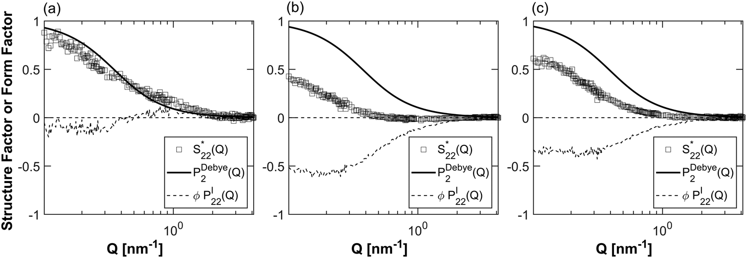
From eqn (6b), the same decomposition can be done for the polymer self-correlation structure factor (S₂₂). The single molecule form factor P^Debye₂ in this case is a Debye fit for Gaussian chains (see ESI† for further detail). Fig. 7 plots the dimensionless polymer structure factor with the single-chain form factor P^Debye₂ and the interchain contribution P^I₂₂ for each polymer. While the PNIPAM self-correlation structure factor barely deviates from the single-chain form factor, the single-chain form factors for PDMAPS and POEGA significantly deviate from the dimensionless partial structure factors, indicating that these polymers experience repulsive polymer–polymer interactions. Since the three polymers have very different chemical structures, it is difficult to separate the effect of polymer chemistry from the effect of the protein on the interchain component P^I₂₂. Notably, PDMAPS and POEGA deviate from the single-chain form factor in a very similar manner. Taken together with the protein–protein structure factors in Fig. 6, it appears that PDMAPS and POEGA have significant interactions with the protein, leading to lower segregation strength between protein and polymer blocks when they are incorporated into an mCherry bioconjugate.

Fig. 7 Single chain and interchain components of the non-dimensionalized polymer–polymer structure factor S₂₂* for (a) PNIPAM, (b) POEGA, and (c) PDMAPS. The single molecule component P^Debye₂ is the Debye form factor for Gaussian chains. The intermolecular component P^I₂₂ is scaled by the volume fraction of polymer.

In addition to the self-correlation structure factors, the cross structure factor S₁₂ directly measures the interaction between protein and polymer, shown in Fig. 5 in black. The cross structure factor varies in both shape and sign across the three polymer chemistries. For PNIPAM, the cross structure factor is negative for low to mid-Q ranges, indicating repulsive interactions between PNIPAM and mCherry. For POEGA, the cross structure factor is weakly negative at low Q compared to PNIPAM–mCherry, but it is positive at mid-Q ranges, suggesting that there are attractive interactions between protein and polymer at intermediate length scales. For PDMAPS, the cross structure factor is negative at low Q, but it is less negative than the PNIPAM cross structure factor. The cross structure factor suggests that the interactions between the two non-ionic polymers and mCherry are very different, which could explain the differences in self-assembly for PNIPAM and POEGA-based bioconjugates. PDMAPS likely has additional electrostatic interactions with mCherry that change the self-assembly behavior when conjugated to mCherry.

Quantifying interactions using real-space correlation functions

To probe the interactions between protein and polymer from a more physically intuitive standpoint, the partial structure factors were inverse Fourier transformed into real space. The partial structure factor as defined in eqn (2) is the Fourier transform of a concentration correlation function between components i and j, Γ_ij(R):⁵³Since the partial structure factor is from experiment, making the null scattering at Q = 0 unobservable, the concentration correlation function can be defined aswhere δϕ_i(R) = ϕ_i(R) − 〈ϕ_i〉 is the local fluctuation of the concentration from the average. Since the scattering intensities obtained from CV-SANS are radial averages of isotropic scattering centers, the inverse Fourier transform of the partial structure factor can be simplified into a 1D sine transform, giving:

Prior to applying the inverse Fourier transform in eqn (9) to the partial structure factors in Fig. 5, the experimental scattering intensities, I(Q), were extrapolated to Q = 0 nm⁻¹ using a Guinier-like analysis and to Q = 50 nm⁻¹ using a flat background of 0 at high Q (see ESI† for more details on the algorithm). It was determined that extrapolation to Q-values above 50 nm⁻¹ did not result in any changes to the inverse Fourier transformed result. In addition, the resulting partial structure factors were smoothed using a robust linear regression over each window of points, with a window size ranging from 5 to 40 points; this step was necessary to suppress the appearance of spurious peaks from Fourier transforming noisy data. The optimal window size was determined by smoothing the data, inverse Fourier transforming it viaeqn (9), and Fourier transforming the result to reconstruct the original partial structure factor. Not all window sizes were able to both smooth the data points and reconstruct the partial structure factor. Actual windows used for smoothing are reported in Table S3 (ESI†). The inverse Fourier transforms of the smoothed partial structure factors are shown in Fig. 8. The factor of V in eqn (9) was omitted to compare dimensionless correlation functions across the three types of polymers. Since the concentration correlation function measures correlations between fluctuations in the local concentration, a positive correlation function does not necessarily imply attractive interactions. For example, negative fluctuations from the average concentration for both protein and polymer would result in a positive correlation function.

Fig. 8 Dimensionless concentration correlation function Γ_ij* between components i and j for (a) PNIPAM/mCherry, (b) POEGA/mCherry, and (c) PDMAPS/mCherry.

The behavior of the protein–protein correlation function reveals that polymer chemistry has a drastic effect on the types of interactions in semidilute aqueous blends of protein and polymer. The nature of the interactions in each system is illustrated in Fig. 9. For PNIPAM–mCherry blends, the dominant interaction between mCherry proteins appears to be depletion (see Fig. 9a). As shown in Fig. 8a, the mCherry–mCherry correlation function Γ₁₁* has a positive peak at around 1.2 nm, which corresponds to the approximate size of mCherry (R_g = 1.56 nm).⁵¹ This suggests that the protein acts like a hard colloid interacting with other proteins in the first coordination shell. This distance can be less than the actual dimensions of the mCherry beta-barrel as shown in Fig. 2d because the mass in the protein is not concentrated at the center of the protein but may be distributed toward the surface.

Fig. 9 Interactions between mCherry and (a) PNIPAM, (b) POEGA, and (c) PDMAPS. PNIPAM drives a depletion interaction between mCherry molecules. POEGA experiences attractive interactions with mCherry molecules, leading to polymer adsorption close to the protein surface. PDMAPS also experiences attractive interactions with mCherry molecules but they are weaker than that of POEGA and driven by electrostatics. PDMAPS also induces depletion interactions between mCherry molecules. The electrostatic surface potential (±5 kT/e_c, with red and blue representing negative and positive values, respectively) at the solvent-accessible surface of mCherry is rendered from the Adaptive Poisson–Boltzmann Solver (APBS) plugin of PyMOL.^54–57 For mCherry and PDMAPS, red represents negative charge and blue represents positive charge. Nonionic polymers are depicted as black.

The PNIPAM–PNIPAM correlation function Γ₂₂* is highly correlated at R = 0 nm and decreases quickly as R increases. The polymer appears to only correlate with itself intramolecularly, which is consistent with a polymer-induced depletion interaction. PNIPAM is also known to form extensive hydration networks, further decreasing its propensity to interact with protein or even other molecules of PNIPAM.⁵⁸ The cross-correlation function Γ₁₂* has a positive peak at R = 0 nm and decreases when Γ₁₁* increases until it reaches a negative well at 1.91 nm. There are two possibilities for the positive correlation at small distances: positive fluctuations away from the average concentration of both polymer and protein or negative fluctuations away from the average concentration of both polymer and protein. If PNIPAM drives a depletion interaction between mCherry proteins, then the latter possibility is more likely, as this means that at small distances less than the radius of gyration of protein, there is less polymer and less protein compared to the bulk solution due to excluded volume and depletion effects. Once distances increase beyond the protein R_g, there is a negative cross-correlation, as polymer is depleted away from the protein surface. The crossover point of the cross-correlation function corresponds to the location of the protein–protein peak at 1.2 nm. The width of this negative well (an estimate of the depletion thickness) is approximately 1.7 nm, which agrees with some theoretical work that in the protein limit, the length scale for depletion is the size of the colloid.^42,43 These results are also consistent with the analysis in Fig. 7, which shows that PNIPAM barely deviates from a Gaussian chain in solution even in the presence of mCherry. Therefore, in the PNIPAM–mCherry system, polymer and protein tend to associate with like molecules rather than each other, which may be why the mCherry-b-PNIPAM block copolymer exhibits self-assembled morphologies over the widest range of concentration and temperature (see Fig. 1).

While the dominant interaction in the PNIPAM–mCherry system appears to be depletion, the POEGA–mCherry correlation functions indicate a different type of interaction (Fig. 8b). While PNIPAM and POEGA are both LCST polymers in water, POEGA has a lower LCST and only has hydrogen bond acceptors in its chain. Here, the mCherry self-correlation function Γ₁₁* is maximized at R = 0 nm, with a second smaller peak at R ≈ 1.97 nm. The most likely explanation for the peak positive correlation at R = 0 nm is the correlation of a molecule of mCherry with itself (i.e. an intramolecular correlation), given that mCherry is a globular protein that cannot occupy the same space as another mCherry protein. In this case, the second peak at 1.97 nm would correspond to correlations with other mCherry proteins in the first coordination shell. The POEGA-POEGA correlation function Γ₂₂* is closer to 0 than the other correlation functions, indicating weak interactions between polymers. It has a peak at 0 nm, like PNIPAM, but it decreases into a small negative well at 1.17 nm. Incidentally, this is between the cross-correlation function Γ₁₂* peak at 0.72 nm and a local minimum in Γ₁₁* at 1.34 nm. This is suggestive of a polymer adsorption layer on the protein surface with about 1 nm thickness. This adsorption layer is smaller than both the radius of gyration (1.56 nm) and cylinder radius (1.506 nm) of mCherry, indicative of a close interaction with the surface exposed residues of the protein, as illustrated in Fig. 9b. In addition, the adsorption layer appears to influence the mCherry self-correlation function, as it leads to a strong intramolecular contribution that is not seen in the PNIPAM–mCherry blend. Moreover, because there is a polymer layer on the protein, the location of the protein first coordination shell shifts outward (1.97 nm) from that of the PNIPAM/mCherry system (1.22 nm). The strong cross-correlation between mCherry and POEGA may explain why mCherry-b-POEGA block copolymers self-assemble over a smaller window of concentrations than mCherry-b-PNIPAM (see Fig. 1). The weaker segregation strength between mCherry and POEGA may also enable the block copolymer to form a cubic Ia3̄d phase, which is not observed for the PNIPAM-based bioconjugate.^34,49

The correlation functions for the PDMAPS–mCherry system in Fig. 8c are more difficult to interpret. The mCherry self-correlation function Γ₁₁* has a peak at 1.7 nm, which is consistent with a coordination shell at the protein radius of gyration, but it is negative at 0 nm. It is possible that the shallow negative well is an artifact from noise in the partial structure factors, given that below the radius of a hard colloid the only allowable self-correlation is intramolecular self-correlation, which should be positively correlated. Of the three sets of scattering data, PDMAPS had the most non-Guinier-like behavior at small Q, which increases the uncertainty on the small Q extrapolation. The PDMAPS self-correlation function Γ₂₂* behaves much like that of PNIPAM but with a weaker magnitude, indicating weaker interactions between polymer chains. The similarities between the polymer and protein self-correlation functions of PNIPAM and PDMAPS suggest that PDMAPS also drives a depletion interaction between mCherry proteins, though it is weaker than for PNIPAM and mCherry. In addition, there is a slight positive cross-correlation Γ₁₂* of PDMAPS with mCherry at 1 nm, indicating some surface interactions between the zwitterionic polymer and the protein (see Fig. 9c). These interactions are much weaker than those experienced between POEGA and mCherry. The PDMAPS–mCherry system may experience electrostatically driven interactions between protein and polymer, which is consistent with the observation that mCherry-b-PDMAPS only self-assembles over a very narrow range of temperatures and concentrations compared to PNIPAM or POEGA-based bioconjugates (see Fig. 1).^34,50

A variable that may affect the interactions between polymer and protein is the hydration number n_H. It has been hypothesized that hydration water, or bound water molecules, can lead to differences in self-assembly among bioconjugates with various polymer chemistries.⁴⁹ To investigate the effect of hydration number, partial structure factors were calculated for a series of hydration numbers ranging from 0 to 10 (Fig. S13, ESI†) and then inverse Fourier transformed into concentration correlation functions. Fig. 10 shows the concentration correlation functions for different hydration numbers for PNIPAM (see Fig. S14, ESI† for other polymers). In all cases, the effect of a higher hydration number is to enhance the correlation between components (whether polymer–polymer or polymer–protein) without changing the overall shape of the correlation as a function of distance. This indicates that any error in estimating the effect of bound hydration water on the scattering profiles water cannot change the specific nature of a polymer–polymer self-interaction or a polymer–protein cross-interaction, but it can change the strength of the interaction. Thus, if hydration number is concentration-dependent, then it may have an effect on the location of phase boundaries and the phases that are observed for each type of mCherry-b-polymer bioconjugate.

Fig. 10 Variation in dimensionless correlation function Γ_ij* with respect to hydration water for (a) PNIPAM/PNIPAM interactions and (b) PNIPAM/mCherry interactions demonstrating that hydration number tunes the strength but not nature of interactions.

Hydration may also be temperature dependent. It is possible that PDMAPS has weaker interactions compared to PNIPAM and POEGA because the PDMAPS/mCherry blends were measured at 35 °C, which is close to the cloud point temperature for this polymer (27.7 °C). In contrast, the other polymer/mCherry blends were measured at 5 °C, which is far away from their respective cloud point temperatures (see Table 1), making it more favorable for water to interact with polymer chains. However, PDMAPS is also a charged UCST polymer, which is governed by different solubility mechanisms compared to POEGA and PNIPAM, which are uncharged LCST polymers. Thus, further conclusions cannot be drawn without collecting CV-SANS data at different temperatures.

Conclusions

The interactions between polymers and proteins in semidilute blends were investigated using contrast-variation SANS (CV-SANS). Three polymers—PNIPAM, POEGA, and PDMAPS—were studied at a volume fraction of 0.05 in solution, with an equivalent volume of the red fluorescent protein mCherry. By varying solvent contrast in a series of SANS measurements, the absolute intensity curves for each protein–polymer set can be decomposed into three constituent partial structure factors per set: polymer–polymer self-correlation, protein–protein self-correlation, and protein–polymer cross-correlation. These structure factors were inverse Fourier transformed into real-space concentration correlation functions that provided information on the nature and strength of interactions between protein and polymer. It is apparent that polymer chemistry has a profound effect on interactions between proteins, between polymers, and between polymers and proteins. The PNIPAM–mCherry behavior is consistent with a system dominated by polymer-induced depletion forces between proteins with minimal cross-correlation. In contrast, POEGA appears to form an adsorption layer on the surface of mCherry molecules. The cross-interaction between POEGA and mCherry may explain why mCherry-b-POEGA bioconjugates self-assemble over a narrower range of conditions than mCherry-b-PNIPAM bioconjugates. The PDMAPS–mCherry system appears to have PNIPAM-like depletion interactions as well as cross-interaction between protein and polymer, possibly due to attractive electrostatic forces. The competition between depletion and electrostatic attraction may contribute to the weaker self-assembly exhibited in mCherry-b-PDMAPS bioconjugates. Overall, this work demonstrates that CV-SANS is a powerful tool for probing complex interactions between molecules in a two-component solution system even in the semidilute regime.

Conflicts of interest

There are no conflicts to report.

Acknowledgements

This work was supported by the Department of Energy Office of Basic Energy Sciences Neutron Scattering Program (award number DE-SC0007106). CV-SANS experiments were conducted at the NIST Center for Neutron Research (NCNR) NGB 30 m instrument. Dilute solution SANS experiments for polymer hydration were run at Oak Ridge National Lab (ORNL) EQ-SANS and Bio-SANS instruments. We thank Dr Boualem Hammouda (NCNR), Dr Changwoo Do (ORNL EQ-SANS), and Dr Shuo Qian (ORNL Bio-SANS) for neutron scattering assistance. We thank Tzyy-Shyang Lin, Dr Carolyn Mills, and Dr Michelle Calabrese for assistance with SANS, Fourier transform, and hydration data analysis.

References

1. M. Goldberg, R. Langer and X. Jia, J. Biomater. Sci., 2007, 18, 241–268.
2. W. Hassouneh, S. R. MacEwan and A. Chilkoti, Methods Enzymol., 2012, 502, 215–237.
3. A. E. G. Cass, G. Davis, G. D. Francis, H. A. O. Hill, W. J. Aston, I. J. Higgins, E. V. Plotkin, L. D. L. Scott and A. P. F. Turner, Anal. Chem., 1984, 56, 667–671.
4. M. Kim, M. Gkikas, A. Huang, J. W. Kang, N. Suthiwangcharoen, R. Nagarajan and B. D. Olsen, Chem. Commun., 2014, 50, 5345–5348.
5. G. F. Drevon and A. J. Russell, Biomacromolecules, 2000, 1, 571–576.
6. O. Kirk, T. V. Borchert and C. C. Fuglsang, Curr. Opin. Biotechnol., 2002, 13, 345–351.
7. H. Yamada and M. Kobayashi, Biosci., Biotechnol., Biochem., 1996, 60, 1391–1400.
8. S. D. Minteer, B. Y. Liaw and M. J. Cooney, Curr. Opin. Biotechnol., 2007, 18, 228–234.
9. T. H. Bayburt and S. G. Sligar, Protein Sci., 2003, 12, 2476–2481.
10. J. Ge, E. Neofytou, J. Lei, R. E. Beygui and R. N. Zare, Small, 2012, 8, 3573–3578.
11. G. M. Whitesides and C.-H. Wong, Angew. Chem., Int. Ed. Engl., 1985, 24, 617–638.
12. M. Hambourger, M. Gervaldo, D. Svedruzic, P. W. King, D. Gust, M. Ghirardi, A. L. Moore and T. A. Moore, J. Am. Chem. Soc., 2008, 130, 2015–2022.
13. M. P. Vasquez, J. N. da Silva, M. B. de Souza, Jr. and N. Pereira, Jr., Appl. Biochem. Biotechnol., 2007, 137-140, 141–153.
14. A. J. Russell, J. A. Berberich, G. F. Drevon and R. R. Koepsel, Annu. Rev. Biomed. Eng., 2003, 5, 1–27.
15. S. Jones and J. M. Thornton, Proc. Natl. Acad. Sci. U. S. A., 1996, 93, 13–20.
16. A. R. Freedman, G. Galfre, E. Gal, H. J. Ellis and P. J. Ciclitira, J. Immunol. Methods, 1987, 98, 123–127.
17. B. Hussain, M. Yüce, N. Ullah and H. Budak, in Nanobiosensors, ed. A. M. Grumezescu, Academic Press, 2017, pp. 93–127,  DOI:10.1016/B978-0-12-804301-1.00003-5.
18. J. Banoub and F. Jahouh, Molecular Technologies for Detection of Chemical and Biological Agents, Dordrecht Springer, Netherlands, 2017, pp. 51–87,  DOI:10.1007/978-94-024-1113-3_4.
19. M. T. McBride, S. Gammon, M. Pitesky, T. W. O'Brien, T. Smith, J. Aldrich, R. G. Langlois, B. Colston and K. S. Venkateswaran, Anal. Chem., 2003, 75, 1924–1930.
20. N. Ferrara, K. J. Hillan, H. P. Gerber and W. Novotny, Nat. Rev. Drug Discovery, 2004, 3, 391–400.
21. S. D. Minteer, Enzyme Stabilization and Immobilization, 2010.
22. U. Hanefeld, L. Gardossi and E. Magner, Chem. Soc. Rev., 2009, 38, 453–468.
23. U. T. Bornscheuer, Angew. Chem., Int. Ed., 2003, 42, 3336–3337.
24. S. A. Ansari and Q. Husain, Biotechnol. Adv., 2012, 30, 512–523.
25. R. E. Kontermann, Curr. Opin. Biotechnol., 2011, 22, 868–876.
26. R. Duncan, Nat. Rev. Drug Discovery, 2003, 2, 347–360.
27. S. Jevsevar, M. Kunstelj and V. G. Porekar, Biotechnol. J., 2010, 5, 113–128.
28. R. J. Mancini, J. Lee and H. D. Maynard, J. Am. Chem. Soc., 2012, 134, 8474–8479.
29. J. Broecker, B. T. Eger and O. P. Ernst, Structure, 2017, 25, 384–392.
30. B. Trzebicka, B. Robak, R. Trzcinska, D. Szweda, P. Suder, J. Silberring and A. Dworak, Eur. Polym. J., 2013, 49, 499–509.
31. M. Li, P. De, S. R. Gondi and B. S. Sumerlin, Macromol. Rapid Commun., 2008, 29, 1172–1176.
32. H. Li, A. P. Bapat, M. Li and B. S. Sumerlin, Polym. Chem., 2011, 2, 323–327.
33. A. Huang, G. Qin and B. D. Olsen, ACS Appl. Mater. Interfaces, 2015, 7, 14660–14669.
34. C. N. Lam and B. D. Olsen, Soft Matter, 2013, 9, 2393–2402.
35. X. Dong, A. Obermeyer and B. D. Olsen, Angew. Chem., Int. Ed., 2016, 56, 1273–1277.
36. C. S. Thomas, M. J. Glassman and B. D. Olsen, ACS Nano, 2011, 5, 5697–5707.
37. Z. Wang, E. van Andel, S. P. Pujari, H. Feng, J. A. Dijksman, M. M. J. Smulders and H. Zuilhof, J. Mater. Chem. B, 2017, 5, 6728–6733.
38. D. L. Worcester, Proc. Natl. Acad. Sci. U. S. A., 1978, 75, 5475–5477.
39. C. G. de Kruif and R. Tuinier, Food Hydrocolloids, 2001, 15, 555–563.
40. A. M. Kulkarni, A. P. Chatterjee, K. S. Schweizer and C. F. Zukoski, Phys. Rev. Lett., 1999, 83, 4554–4557.
41. Z. Li and J. Wu, J. Chem. Phys., 2007, 126, 144904.
42. M. Surve, V. Pryamitsyn and V. Ganesan, J. Chem. Phys., 2005, 122, 154901.
43. T. Odijk, Macromolecules, 1996, 29, 1842–1843.
44. D. I. Svergun, S. Richard, M. H. J. Koch, Z. Sayers, S. Kuprin and G. Zaccai, Proc. Natl. Acad. Sci. U. S. A., 1998, 95, 2267–2272.
45. M. H. G. Duits, R. P. May, A. Vrij and C. G. D. Kruif, J. Chem. Phys., 1991, 94, 4521–4531.
46. M. Shibayama, T. Matsunaga, T. Kusano, K. Amemiya, N. Kobayashi and T. Yoshida, J. Appl. Polym. Sci., 2014, 131, 39842.
47. S. Miyazaki, H. Endo, T. Karino, K. Haraguchi and M. Shibayama, Macromolecules, 2007, 40, 4287–4295.
48. M. Takenaka, S. Nishitsuji, N. Amino, Y. Ishikawa, D. Yamaguchi and S. Koizumi, Macromolecules, 2009, 42, 308–311.
49. D. Chang, C. N. Lam, S. Tang and B. D. Olsen, Polym. Chem., 2014, 5, 4884–4895.
50. D. Chang and B. D. Olsen, Polym. Chem., 2016, 7, 2410–2418.
51. C. N. Lam, D. Chang, M. Wang, W.-R. Chen and B. D. Olsen, J. Polym. Sci., Part A: Polym. Chem., 2016, 54, 292–302.
52. B. Hammouda, Probing Nanoscale Structures: The SANS Toolbox, NIST, Gaithersburg, MD, 2010.
53. R.-J. Roe, Methods of X-ray and Neutron Scattering in Polymer Science, Oxford University Press, New York, 2000.
54. N. A. Baker, D. Sept, S. Joseph, M. J. Holst and J. A. McCammon, Proc. Natl. Acad. Sci. U. S. A., 2001, 98, 10037–10041.
55. E. Jurrus, D. Engel, K. Star, K. Monson, J. Brandi, L. E. Felberg, D. H. Brookes, L. Wilson, J. Chen, K. Liles, M. Chun, P. Li, D. W. Gohara, T. Dolinsky, R. Konecny, D. R. Koes, J. E. Nielsen, T. Head-Gordon, W. Geng, R. Krasny, G.-W. Wei, M. J. Holst, J. A. McCammon and N. A. Baker, Protein Sci., 2018, 27, 112–128.
56. T. J. Dolinsky, J. E. Nielsen, J. A. McCammon and N. A. Baker, Nucleic Acids Res., 2004, 32, W665–W667.
57. T. J. Dolinsky, P. Czodrowski, H. Li, J. E. Nielsen, J. H. Jensen, G. Klebe and N. A. Baker, Nucleic Acids Res., 2007, 35, W522–W525.
58. Y. Okada and F. Tanaka, Macromolecules, 2005, 38, 4465–4471.

---

Footnotes

† Electronic supplementary information (ESI) available. See DOI: 10.1039/c9sm00766k

‡ A. H. and H. Y. contributed equally to this work.

---