
 Open Access Article
 This Open Access Article is licensed under a
 Creative Commons Attribution 3.0 Unported Licence
Hierarchical modelling of polystyrene melts: from soft blobs to atomistic resolution
Guojie
Zhang
 ab,
Anthony
Chazirakis
cd,
Vagelis A.
Harmandaris
*cd,
Torsten
Stuehn
b,
Kostas Ch.
Daoulas
*b and
Kurt
Kremer
*b
ab,
Anthony
Chazirakis
cd,
Vagelis A.
Harmandaris
*cd,
Torsten
Stuehn
b,
Kostas Ch.
Daoulas
*b and
Kurt
Kremer
*b
aInstitute for Systems Rheology, Advanced Institute of Engineering Science for Intelligent Manufacturing, Guangzhou University, 510006 Guangzhou, China. E-mail: guojie.zhang@gzhu.edu.cn
bMax Planck Institute for Polymer Research, Ackermannweg 10, 55128 Mainz, Germany. E-mail: daoulas@mpip-mainz.mpg.de; kremer@mpip-mainz.mpg.de
cDepartment of Mathematics and Applied Mathematics, University of Crete, GR-71409 Heraklion, Crete, Greece. E-mail: harman@uoc.gr
dInstitute of Applied and Computational Mathematics, IACM/FORTH, Heraklion, Greece
First published on 28th November 2018
Abstract
We demonstrate that hierarchical backmapping strategies incorporating generic blob-based models can equilibrate melts of high-molecular-weight polymers, described with chemically specific, atomistic models. The central idea is first to represent polymers by chains of large soft blobs (spheres) and efficiently equilibrate the melt on large scales. Then, the degrees of freedom of more detailed models are reinserted step by step. The procedure terminates when the atomistic description is reached. Reinsertions are feasible computationally because the fine-grained melt must be re-equilibrated only locally. We consider polystyrene (PS) which is sufficiently complex to serve method development because of stereo-chemistry and bulky side groups. Our backmapping strategy bridges mesoscopic and atomistic scales by incorporating a blob-based, a moderately coarse-grained (CG), and a united-atom model of PS. We demonstrate that the generic blob-based model can be parameterised to reproduce the mesoscale properties of a specific polymer – here PS. The moderately CG model captures stereo-chemistry. To perform backmapping we improve and adjust several fine-graining techniques. We prove equilibration of backmapped PS melts by comparing their structural and conformational properties with reference data from smaller systems, equilibrated with less efficient methods.
1 Introduction
A molecular structure based understanding of properties of technologically or experimentally relevant polymer melts, or dense solutions, still poses significant scientific challenges. Computational studies of structure–process–property relationships in polymer liquids often require the consideration of atomistic details, while at the same time many fundamental scientific questions and important technological applications can be addressed only for high molecular-weight (MW) polymers. These simultaneous requirements create major challenges at high polymer concentrations, e.g. concentrated solutions and melts. For typical polymerisation degrees in industrial applications, the average spatial extension of random-walk-like chains lies1 between 10 and 100 nm. In concentrated polymer liquids these fractal “threads” strongly interdigitate. To avoid finite-system size effects, simulations must consider samples with dimensions that are at least two times larger than the root-mean-square end-to-end distance of the molecules, Re. This minimum requirement, however, already leads to samples that contain hundreds or even thousands of polymers, which easily corresponds to many millions of atomistic degrees of freedom.To demonstrate that samples spanning only a couple of Re have a large number of particles, it is useful to consider the following scaling estimate.2,3 The number of polymers crossing the volume of a test chain is proportional to 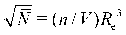 , where n and V are, respectively, the total number of chains and volume of the system. In polymer melts Re2 ≃ Nklk2, where Nk is the number of Kuhn segments in a chain and lk the length of a single Kuhn segment. The chain density is expressed through the volume per single Kuhn segment, υk, as n/V = 1/υkNk. Therefore
 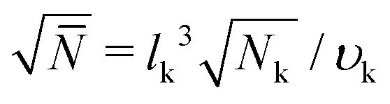 . Because υk/lk2 defines the packing length p, lk3/υk = lk/p. lk/p plays a key role for rheological properties and for many polymers4lk/p ∼ 1–10. Since the molecular mass of a Kuhn segment is typically a few hundred g mol−1, for polymers with high MW5Nk ∼ 103 and thus
 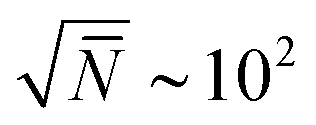 . In other words, simulations of melts with long chains must handle samples where the basic subvolume, ∼Re3, already contains one hundred chains (at least). The overlapping polymers are strongly entangled6 and their relaxation times are prohibitively long. Their equilibration with atomistic molecular dynamics (MD) is unfeasible even when using massively parallel simulations. Therefore approaches circumventing the slow relaxation path of physical dynamics are of significant interest. Well equilibrated atomistic systems are indispensable initial conditions to simulation studies of atomistic long-chain polymer melts. Various strategies are available, including advanced connectivity altering Monte Carlo (MC) algorithms7,8 and methods based on hierarchical multiscale modelling.
Hierarchical multiscale modelling involves multiple scales of description9–17 and offers a powerful concept for tackling large system sizes and protracted equilibration times. The central idea is to benefit from scale separation: in polymers long-wavelength behavior often follows universal laws18 that incorporate chemistry-specific information into a few parameters. Therefore, one can initially eliminate microscopic features hampering equilibration and prepare samples reproducing only mesoscopic conformational and structural properties. These samples serve as “blueprints” for reinserting the missing microscopic features without disturbing long-wavelength properties. The reinsertion is computationally feasible because only local re-equilibration is required. Two major strategies realise this idea: configuration assembly and hierarchical backmapping.
Configuration assembly14,19–22 algorithms construct the initial sample by putting together polymer chains under a fixed average density. Implementations vary in details, but in all cases chains are generated to reproduce prescribed distributions of conformations. If the ensemble is generated as an ideal gas of chains, important long-wavelength structural properties, such as the correlation hole effect,18 are missing. Therefore, one must reduce the large density fluctuations of the ideal gas of chains and introduce some interchain correlations through chain packing schemes.19,20 Subsequently local conformations and liquid packing are recovered through a “push off” procedure, which gradually19 reinserts the microscopic excluded volume into the ensemble. The strategy has been successful with generic19,20 and chemistry specific14,21,22 microscopic models. However, the postulative construction of starting configurations is a drawback. The assumption that polymers have ideal random-walk-like conformations in melts is only approximately true.23,24 Examples of deviations from ideal random-walk statistics are found in the power-law decay of bond–bond correlations23 and statistics of polymer knots.25 Predicting conformations for polymers with complex architecture (star-like or branched) and systems that are inhomogeneous or multicomponent is even less straightforward. Furthermore, the computational costs at the stage of chain packing increase with molecular weight.
Hierarchical backmapping is a more general approach, taking advantage of a general concept originating from renormalization group theory in critical phenomena. The material is described at several “nested” length scales, introducing a sequence of coarse-grained (CG) models. The sequence is terminated by the microscopic model. Because the sample is equilibrated at the largest length scale with standard simulations (handling the crudest CG model), long-wavelength properties are not postulated but follow from a rigorous statistical–mechanical framework. The molecular details resolved by the next model are reinserted through local sampling of configuration space. Repeating the procedure, one descends the hierarchy of models, step by step, until the microscopic description is reached. The efficiency increases significantly22,26–31 when the hierarchy includes soft models, i.e. models where the strength of non-bonded interactions is comparable to the thermal energy.
Blob-based models27,32–47 offer a straightforward way to construct hierarchies of CG representations: Nb monomers of a microscopically-resolved subchain are lumped into a single soft blob (sphere), so that polymers are represented by chains of blobs. Varying Nb generates a family of models with different resolutions. Hierarchical backmapping using blob-based models has been successful in equilibrating high-molecular-weight polymer melts27,47 and blends48 described with generic (bead-spring like) microscopic models. The equilibrated samples typically contained 103 chains, comprised of a few thousands of beads. The method is not limited to these examples – the computational costs of the procedure are not affected by chain length and are, roughly, proportional only to the volume of the system.27 Yet, the question of whether hierarchical strategies with blob-based models can equilibrate melts described with chemically-specific atomistic models remains, so far, open. Concerns regarding this point have been expressed in the literature.22
Here we address this question and demonstrate that hierarchical strategies with generic blob-based models can equilibrate melts of actual polymers, described with chemically-specific atomistic models. As an illustration we develop a hierarchical backmapping method which equilibrates large atomistically-resolved samples of polystyrene (PS) melts. PS is a basic commodity material and is well-suited for method development: it is well studied experimentally and theoretically, and is a sufficiently complex polymer, where molecules have tacticity and bulky units (benzene rings). To descent the hierarchy of scales, from coarse to atomistic, our backmapping strategy incorporates a blob-based,39,43 a moderately49,50 CG, and a united-atom49,51 (UA) model of PS. We demonstrate that a generic blob-based model39,43,47 can describe the rather complex PS melt accurately enough to allow backmapping. To perform backmapping within the hierarchy of chemically-specific models, we improve and adjust several reinsertion techniques.14,19,20 These methodological issues are also discussed in the paper.
2 Hierarchy of models
Our hierarchical strategy for equilibrating large samples of high-molecular-weight polymer melts, described with atomistic detail, requires several models covering a broad range of length scales: from atomistic, to moderately CG, up to mesoscopic. In this section we present the models used for the hierarchical description of PS.2.1 Atomistic model
On the atomistic level we describe PS through a united atom (UA) model based on the TraPPE-UA force field.52 Details can be found in previous studies,49,51,53 so we mention here briefly that in this UA model each PS monomer is represented by groups of eight UAs (see Fig. 1(a)). The full interaction potential of atomistic PS involves bonded and non-bonded terms. Angular and torsional potentials are introduced for the aliphatic backbone, while keeping the lengths of the bonds fixed. Improper dihedral potentials are used to keep the phenyl ring planar and to maintain the tetrahedral configuration around the sp3-hybridised carbon connected to the phenyl ring. Non-bonded interactions between UAs are captured by pairwise Lennard-Jones (LJ) potentials.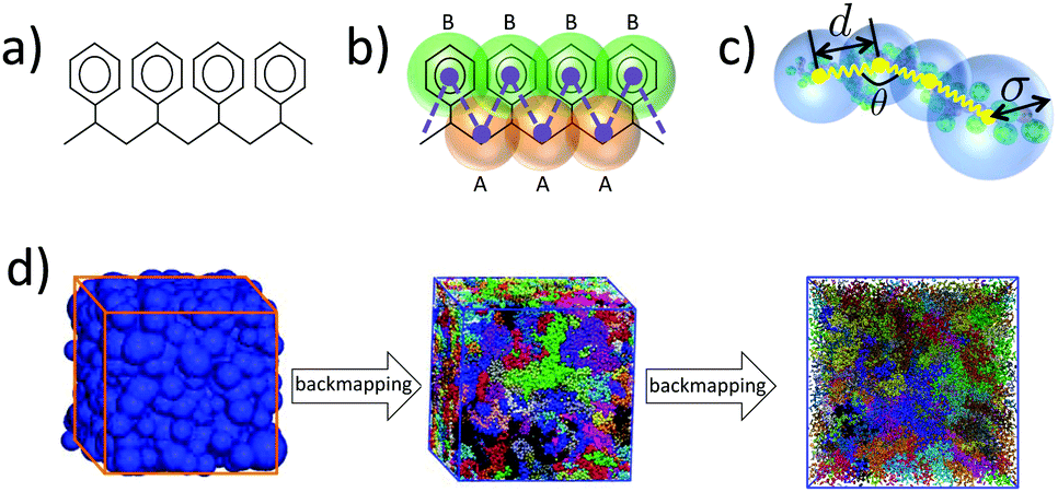 | ||
| Fig. 1 PS models used during hierarchical backmapping: (a) the united atom (UA) model; (b) the moderately coarse-grained (CG) model, A-type beads (orange) represent a CH2 group and half of its two neighboring CH groups along the aliphatic backbone, while B-type beads (green) describe the phenyl rings; and (c) the blob-based (BL) model constructed by grouping a large number of beads of the moderately CG model into soft spheres. (d) Summary of basic steps of the hierarchical backmapping. An equilibrated blob-based configuration of PS is first obtained from efficient Monte Carlo (MC) simulations and the degrees of freedom of the moderately CG model are reinserted into this configuration. The equilibrated PS melt obtained after this reinsertion is further backmapped on the UA description. The snapshots show an equilibrated PS melt with 100 chains and 480 monomers per chain (MW = 50 kDa) at three different resolutions. | ||
Despite the fact that we are using a UA model, it is rather straightforward to obtain and simulate all-atom systems by adding hydrogens to the UA PS configurations. However, since the chosen UA PS model has been extensively used and examined before, we choose to represent the atomistic PS chains in the UA description.
2.2 Moderately coarse-grained model
We employ a moderately (quantitative) CG model that has been derived14,53 from the UA description presented in Section 2.1. The model and the procedure used to obtain the CG force field have been elaborated elsewhere.14,49 In summary, each PS monomer is mapped on two effective beads, “superatoms”, A and B (see Fig. 1(b)). Bead A represents the CH2 unit of a PS monomer and half of each of the two neighboring CH groups along the chain backbone. Bead B stands for the phenyl ring. The sizes and masses of A and B superatoms are σA = 4.1 Å, σB = 5.2 Å, mA = 27 amu, and mB = 77 amu, respectively. Such a model is capable of providing quantitative predictions about both static and dynamic properties of PS systems. In addition, for the moderately CG model we define: (a) a characteristic length scale as the average bead size, i.e., σCG = (σA + σB)/2 = 4.65 Å, and (b) a characteristic time scale,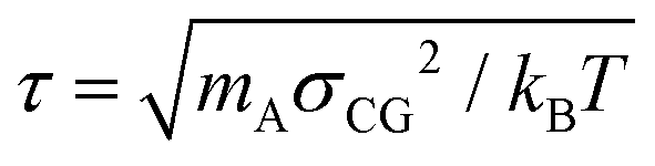 (kBT is the thermal energy).
This CG scheme can describe tacticity of PS chains without introducing side groups, by classifying the B beads into four subtypes. In total, the bonded part of the CG force field includes one bond, but four “alternative” angular and dihedral interaction potentials. The specific sequence of potentials chosen for angular and dihedral interactions along the backbone of a moderately CG chain depends on the tacticity of the atomistic PS molecule it represents.
Nonbonded interactions are described through pair LJ-like, n–m potentials Uα,β(r), where r is the distance between two interacting superatoms. The powers and parameters used in Uα,β(r) depend on the type α and β of the interacting superatoms, i.e. a bead can be A type or belong to one of the four B types. Non-bonded interactions are deactivated for those beads that belong to the same chain and are closer neighbours than (1,5). The details and the parameters of the force-field can be found elsewhere.14,53
The accuracy of the moderately CG model in predicting quantitatively the properties of PS melts has been verified through extensive investigations.14,53 Moreover it was recently demonstrated54 that the moderately CG model is transferable to the crystalline phase of syndiotactic PS. Specifically, it reproduces the crystallisation temperature and stabilises the main α and β polymorphs. For the purposes of our backmapping scheme, the fine structure of the CG model presents significant advantages because it facilitates the subsequent reinsertion of the degrees of freedom of the UA description.
2.3 Blob-based coarse-grained model
The connectivity of soft-sphere chains is described32,39,40,43 using bond, Vb, and angular, Vθ, potentials, defined as:
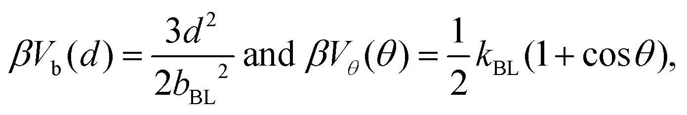 | (1) |
The fluctuations of the radius, σ, of a sphere are controlled by a “self-interaction” potential, Vs(σ), similar to the Flory free energy.55 This potential is defined as:
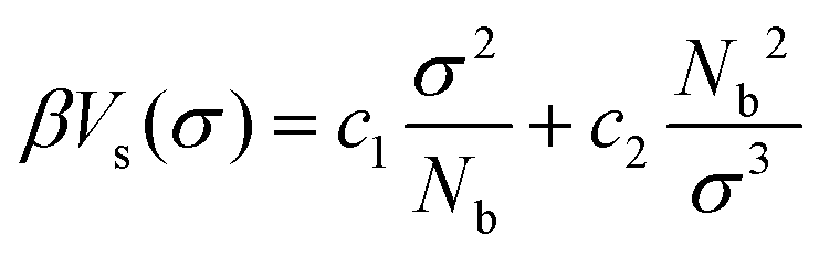 | (2) |
The first term in eqn (2) has entropic origin and balances the swelling induced by the second term, which implicitly accounts for binary intramolecular interactions between the Nb superatoms underlying the blob. In previous studies27,39,43,47 the interactions controlling the fluctuations of σ were augmented by a term proportional to 1/σ6 (following Lhuillier56). In the first implementation of the soft-sphere model39 the 1/σ6 term enabled the description of a broad range of concentration regimes, e.g. dilute solutions. However, in melts the 1/σ6 term is significantly smaller than the 1/σ3 term57 and thus can be omitted.
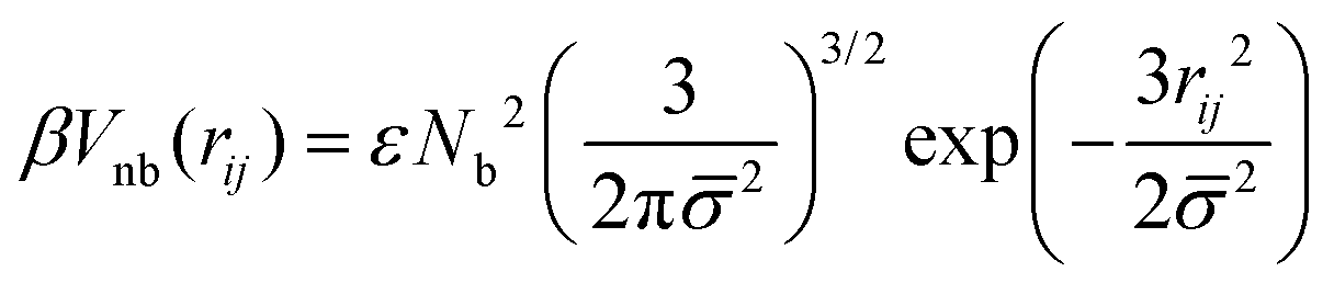
The effective non-bonded interactions between two spheres, i and j, are described by a Gaussian potential:
 | (3) |
![[small sigma, Greek, macron]](https://www.rsc.org/images/entities/i_char_e0d2.gif) 2 = σi2 + σj2, and ε controls the strength of repulsion.58βVnb(rij) is obtained by approximating the interactions of superatoms underlying different spheres by binary repulsive collisions and is proportional to the overlap of two Gaussian clouds. Each of these clouds describes the average distribution in space of superatoms with respect to the COM of the subchain they belong to.
2 = σi2 + σj2, and ε controls the strength of repulsion.58βVnb(rij) is obtained by approximating the interactions of superatoms underlying different spheres by binary repulsive collisions and is proportional to the overlap of two Gaussian clouds. Each of these clouds describes the average distribution in space of superatoms with respect to the COM of the subchain they belong to.
The soft-sphere model of the PS is motivated by simple arguments from polymer physics. The model aims to capture long-wavelength conformational and structural properties of PS melts accurately enough for performing backmapping at one state point. In this work, we define state points using the density of the blobs ρblob = nNBL/V and temperature T. Due to the simple Gaussian-potential approximation used for the non-bonded interactions, we do not expect that various thermodynamic properties of polystyrene, e.g. the equation-of-state, can be well approximated within our soft-sphere model, on the level of the blob description. The reinsertion of atomistic details corrects the thermodynamic inconsistencies.
To sample the configurational space of PS melts described with the soft-sphere model, we benefit from an efficient Monte Carlo (MC) algorithm based on three types of moves: (i) random change of sphere size, (ii) random sphere displacement, and (iii) slithering snake (reptation). A detailed presentation of the method can be found elsewhere.43 We summarise that the computational efficiency stems from a special particle-to-mesh calculation of nonbonded interactions, which avoids neighbor lists.27,43
At the same time, Nb must be smaller than the entanglement length, Ne, for the final backmapping step. When soft-sphere chains are substituted by the moderately CG polymers, the liquid structure and chain conformations in the melt must be relaxed on scales smaller or comparable to the average blob diameter. The condition Nb < Ne warrants that this relaxation is achieved through fast Rouse-like dynamics of short subchains and is not affected by surrounding topological constraints.27 Had we employed a hierarchy with several blob-based models,27 the condition Nb < Ne would apply only to the last, highest resolution, blob-based model (where the reinsertion of the moderately CG description is performed). Depending on the method used to extract the entanglement length, simulations of PS have reported Ne in the range of 100–200 monomers, which is equivalent to 200–400 superatoms.49 These results agree with experiments.62–64 Therefore, we explore different resolutions satisfying the condition Nb ≤ 200. The entanglement time in the moderately CG model is τe ≃ 4 × 10⁴τ.
For each trial Nb, the parameters c1, c2, bBL, kBL, and ε are determined using typical structure-based (or Inverse Boltzmann) coarse-graining.9,13,65 The parameters are chosen so that the probability distributions PBL(σ), PBL(d), and PBL(θ), as well as the pair-correlation function, gBL(r), of the centers of the spheres in blob-based PS melts reproduce closely their counterparts in reference samples described by the moderately CG model. These reference samples contain 50 chains with NCG = 960 superatoms and were equilibrated through a variant14 of the configuration-assembly method proposed by Auhl et al.19 and long CG molecular dynamics simulations. The density of chains in the reference samples is n/V = 1.17 × 10⁻² chains per nm3 and the temperature is set to T = 463 K. In the moderately CG reference samples, the polymers are partitioned into subchains with Nb superatoms. The length of the chains in the reference samples restricts the Nb that can be considered here to a limited set of values, to have an integer number of subchains, i.e. under the condition Nb ≤ 200, we try Nb = 192, 160, 120, and so on. After the subchains are identified, we calculate the distributions of: (i) the gyration radii of subchains, Pref,BL(Rg); (ii) the distance between the COMs of subchains sequential in the same PS molecule, Pref,BL(d); and (iii) the angles between two vectors joining the COM of a subchain with the COMs of the preceding and the succeeding subchain, Pref,BL(θ) (cf.Fig. 1(c)). The pair distribution function of the COMs of subchains, gref,BL(r), serves as the counterpart of gBL(r).
With the reference distributions in hand, the parameters of the soft-sphere model are optimised through an iterative procedure which simultaneously minimises four merit functions, defined66 as:
 | (4) |
To start the iterative procedure, the initial values of bBL and kBL are obtained by fitting the Boltzmann distributions of the potentials Vb(d) and Vθ(θ) from eqn (1) to the reference distributions Pref,BL(d) and Pref,BL(θ), respectively. The parameters c1 and c2 are obtained in a similar way by fitting the Boltzmann distribution of the potential Vs(σ), eqn (2), to Pref,BL(Rg). We emphasise that this first estimate of the parameters is approximate, because it assumes that the distributions are not correlated. A first-guess value for ε can be obtained from c2. To first order, the two parameters can be related to each other by equating the potential c2Nb2/σ3 (cf.eqn (2)), which captures the effect of the repulsion between intramolecular superatoms, to the “self-interaction” of a Gaussian density distribution. The latter is given by βVnb(0)/2; the prefactor 1/2 avoids double counting. This approximation leads to c2 = (ε/2)(3/4π)3/2.
To perform the first iteration step, cf.Fig. 2, we consider the soft-sphere model with the initial values of parameters. The number of blobs in the soft-sphere chains equals the number of subchains used to partition the moderately CG molecules in the reference samples. The melt has n = 100 soft-sphere chains and the volume is chosen such that n/V matches the chain density in the reference systems. The temperature does not appear explicitly in the soft-sphere model, because all interactions in eqn (1) and (2) are scaled by the thermal energy. The melt is equilibrated using particle-to-mesh MC and the distribution function PBL(σ) is extracted to calculate ΔPBL(σ). The parameters c1 and c2 are increased or decreased by 5% and a new simulation is performed. The procedure is repeated until ΔPBL(σ) reaches a minimum value. The configurations from the simulation with the last optimised c1 and c2 are used to calculate ΔPBL(d). The parameter bBL is modified until ΔPBL(d) reaches a minimum. The same procedure is repeated for kBL and ε; the corresponding merit functions are ΔPBL(θ) and ΔgBL(r), cf.Fig. 2. After updating all parameters, we commence a new iteration step. We recalculate ΔPBL(σ) and improve c1 and c2 by minimising again ΔPBL(σ). Subsequently, the remaining parameters are improved, as in the first iteration step. Iteration steps are repeated (e.g. by about five circles in our case) until the minimum values of all merit functions, Δf(x), saturate.
 | ||
| Fig. 2 Procedure used to parameterise the blob-based model of polystyrene melts. | ||
Through exploratory studies we find that the simple soft-sphere model can be parameterised to reproduce static properties of the reference PS melt when Nb ≳ 120. Backmapping a soft-sphere model with the smallest possible Nb is preferable, because this procedure requires shorter relaxation times of reinserted microscopic details. Therefore, in this study we work with Nb = 120; that is, each blob corresponds to 120 CG superatoms or 60 PS monomers.
2.4 Validation of the soft-sphere model
We illustrate that the melts equilibrated with the soft-sphere model indeed describe structural and conformational properties of PS melts on length scales comparable to or larger than the size of the blobs. For Nb = 120, the four panels of Fig. 3 present the distributions PBL(σ), PBL(d), and PBL(θ), as well as the pair distribution function, gBL(r), for a melt of soft-sphere chains (lines) and reference samples (symbols). The agreement of the curves is remarkable. As will be demonstrated in the following, the small deviations observed in the plots do not propagate into the properties of backmapped PS samples. | ||
| Fig. 3 For a PS melt of soft-sphere chains corresponding to Nb = 120, the lines show the probability distributions of (a) the sphere radius, σ, (b) the bond length, d, between spheres, and (c) the angle, θ, between successive bonds. The reference distributions calculated for moderately CG melts of PS are plotted with symbols. (d) For the same melt, the pair distribution function gBL(r) of the centers of the soft spheres (lines) is compared with the pair distribution of the COMs of the subchains with Nb = 120 superatoms (symbols). | ||
Fig. 4(a) and (b) examine the accuracy of the soft-sphere model on scales comparable to the size of the entire PS chain. Fig. 4(a) presents for the soft-sphere model (lines) and reference samples (symbols) the intermolecular part ginter,BL(r) of the pair distribution functions plotted in Fig. 3(d). In both curves, the correlation holes of subchains (evident depletion at small distances) and of entire PS chains (shallow depletion towards tails) can be identified. The two ginter,BL(r) match each other closely, even in their long tails, demonstrating that the blob-based model captures the melt structure on large scales.
 | ||
| Fig. 4 (a) The line shows the intermolecular part, ginter,BL(r), of the pair distribution function of the centers of the blobs in PS melts of soft-sphere chains, corresponding to Nb = 120. Symbols present ginter,BL(r) of COMs of subchains with Nb = 120 superatoms, calculated from the reference samples of moderately CG melts of PS. (b) A normalised internal distance plot, RBL2(s)/s, calculated for PS melts of soft-sphere chains corresponding to Nb = 120 is shown with a line. Symbols present the internal distance plot calculated for the COMs of subchains with Nb = 120 superatoms in the reference samples. | ||
To compare polymer conformations in melts described by the soft-sphere and moderately CG models we employ the internal distance plot, which is a very sensitive conformational descriptor.19 Its general definition for a system containing nc chains, each with N repeat units, reads:67
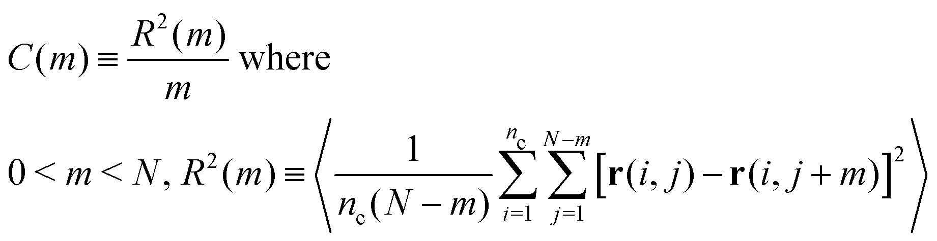 | (5) |
In eqn (5), r(i,j) stands for the position vector of the j-th repeat unit of the i-th chain and angular brackets denote an average over system configurations. The parameter m stands for the “chemical distance” of two repeat units on the same chain, i.e. it expresses the number of repeat units comprising the chain contour between the two considered units. The general definitions of R2(m) and m in eqn (5) are adjusted to the considered chain model. In the soft-sphere model, R2(s) ≡ RBL2(s) is the mean-square distance between the centers of two spheres in the same chain; m ≡ s is the number of spheres between these two blobs along the chain contour. To compare the soft-sphere model with reference data, in our specific case, RBL2(s) in moderately CG melts is defined as the mean-square distance between the COMs of two subchains with Nb = 120 superatoms, belonging to the same molecule. s is the number of intramolecular subchains between them. Fig. 4(b) compares RBL2(s)/s in PS melts described by the soft-sphere (lines) and moderately CG (symbols) models. For large s the plots follow each other closely; for blobs, located near each other along the chain, the relative deviation is at most 3.7%. The internal distance plot demonstrates the accuracy of the soft-sphere model in describing conformational properties on the scale of entire chains.
3 Hierarchical backmapping strategy
3.1 Systems studied
The hierarchical scheme described in the previous section can be applied to systems of any molecular weight for a given density. In practice, for fixed pressure and temperature, the density of the polystyrene becomes chain-length independent for polymerisation degrees larger than about 50–100 monomers.49 Therefore we expect that the soft-sphere model, developed in the previous section, is transferable to PS melts with arbitrarily long chains. However, for the purposes of method development, we set here as a goal the equilibration of atomistic PS melts comprised of n = 100 chains with N = 480 repeat units, which corresponds to a molecular weight of M = 50 kDa. These molecules are equivalent to moderately CG PS molecules with NCG = 960 superatoms and soft-sphere chains with NBL = 8 blobs each. These are the chain lengths for which the soft-sphere model is parameterised and for which reference samples are available14 (cf. Section 2.3.2). Having the same chain lengths in backmapped and reference samples simplifies the validation of the equilibration. The temperature in the backmapped and reference melts is T = 463 K, which is a typical processing temperature for PS.3.2 Backmapping the blob-based model to the chemically specific coarse-grained model
The reinsertion of the degrees of freedom of the chemically specific CG model into equilibrated soft-sphere PS melts is conceptually similar to the strategy developed earlier27 for generic microscopic (bead-spring) models. Technically, however, the backmapping of the chemically specific CG model is more involved, due to the more complex CG force field. The technicalities of the different backmapping steps are presented below.Introducing moderately CG PS molecules: every soft-sphere chain in the melt is replaced by a moderately CG PS molecule in a matching conformation. Specifically, the COM and the radius of gyration (squared) of each subchain with Nb superatoms in the reinserted molecule must match the COM and the radius (squared) of the corresponding blob in the soft-sphere chain. We generate each moderately CG PS molecule in the vicinity of the blob-based chain it must replace (the exact location is not critical). Setting the first bead of a generated molecule to A type, the remaining beads are added stepwise. A and B beads alternate. In this work, we assign randomly to each B bead one of the four subtypes (cf. Section 2.2) to make PS chains atactic. The length, bond angle, and torsional angle of the bond connecting the added superatoms to the part of the molecule that has been already constructed are randomly drawn from Boltzmann distributions. Each distribution depends on the appropriate bonded potential. Once the PS molecules are generated, we associate27 with each subchain two external potentials: βVcm,i = kcm(ri − Rcm,i)2 and βVg,i = kg(σi2 − Rg,i2)2. Here Rcm,i and Rg,i2 are the COM and squared radius of gyration of the i-th reinserted subchain, respectively. These potentials affect all superatoms in the i-th subchain, because Rcm,i and Rg,i depend on the coordinates of all these superatoms. The parameters controlling the strength of the external potentials are empirically set to kcm = 100kBT/σCG2 and kg = 100kBT/σCG4. With the external and bonded potentials simultaneously activated (non-bonded potentials are turned off), the configuration of generated moderately CG molecules is subjected to NVT MD simulation, using the Langevin thermostat. This simulation “drives” every molecule into the corresponding soft-sphere chain. At this stage the molecules do not interact with each other, therefore the simulation takes negligible time.
Recovering the microscopic excluded volume: after the soft-sphere chains are replaced by the moderately CG PS molecules, we remove the external potentials and gradually activate27 the non-bonded interactions between superatoms. For this purpose we use a “push-off” MD procedure19,20 which removes overlaps between reinserted superatoms and recovers the original excluded volume characterising the potentials Uα,β(r). We summarise here the main features of the push-off protocol; details are provided in the Appendix.
The potentials are “force-capped” according to the rule:
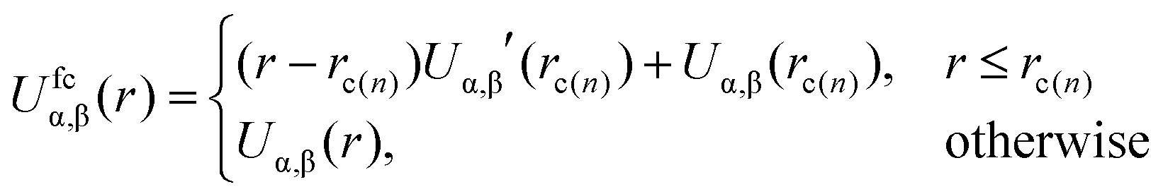 | (6) |
Here rc(n) is the force-capping radius and the original interactions are recovered when rc(n) → 0. The push-off is accomplished in 100 cycles; each of them comprises a change in rc(n) and local relaxation through a short MD simulation. For those beads that are not intramolecular (1,5) neighbours, we decrease rc(n) by a small step at the beginning of each cycle. For intramolecular (1,5) neighbours, rc(1,5) is adjusted in a special way in order to avoid significant distortions of polymer conformations during the push-off. To modify rc(1,5) in the beginning of each cycle, we use an approach similar to the one developed for generic microscopic models.20 Namely, we quantify conformational distortions using the descriptor:
 | (7) |
The MD push-off procedure lasts about 20τ which is a negligible fraction of τe; about 0.05%. In practice, this run takes less than a day on 32 processors of a typical supercomputer.
Local re-equilibration: once the excluded-volume interactions are recovered, the moderately CG PS melt is locally re-equilibrated through a standard MD simulation, which lasts about one τe. This is the most computationally demanding part of our procedure. To give a feeling for the CPU resources that are typically required for re-equilibration, we mention that it takes about 32 days using the ESPResSo++ package68 (version 1.9.5) on 256 Xeon cores with a frequency of 3.0 GHz. We observe that the local re-equilibration of PS melts for ∼τe is about an order of magnitude slower – in terms of the required CPU time – compared to melts described with generic microscopic bead-spring models.27 The protracted computations are not related to the backmapping strategy but are due to the complexity of the chemically-specific force-field. Because the largest relaxation time is determined by τe, the CPU time required by our backmapping procedure does not depend on chain length and is proportional only to system volume.27 In contrast, the relaxation time in brute-force MD simulations is proportional to the reptation time, given by τrep ≃ τe(N/Ne)3; to make a simple scaling argument we use the approximate cubic power law of the initial reptation theory.6,69 The moderately CG PS melts considered here are only weakly entangled: based on the largest reported value Ne = 400 (cf. Section 2.3.2) we obtain N/Ne ≃ 2.4. The estimate for τrep demonstrates that to equilibrate even this system, brute-force MD simulations would require about a year of continuous running (using the same number of processors). Melts with slightly longer PS chains are entirely out of reach of brute-force MD simulations.
3.3 Validating backmapping of the moderately coarse-grained PS melts
We demonstrate the equilibration of backmapped moderately CG melts of PS by monitoring characteristic conformational and structural properties on local and global length scales. These properties are compared with their counterparts calculated for the reference samples. As a first simple test, we present in Fig. 5(a) and (b) the probability distributions of the bond angle and the torsional angle, PCG(θ) and PCG(ϕ). The data obtained for the backmapped melts (lines) are on top of the distributions (symbols) calculated for the reference samples.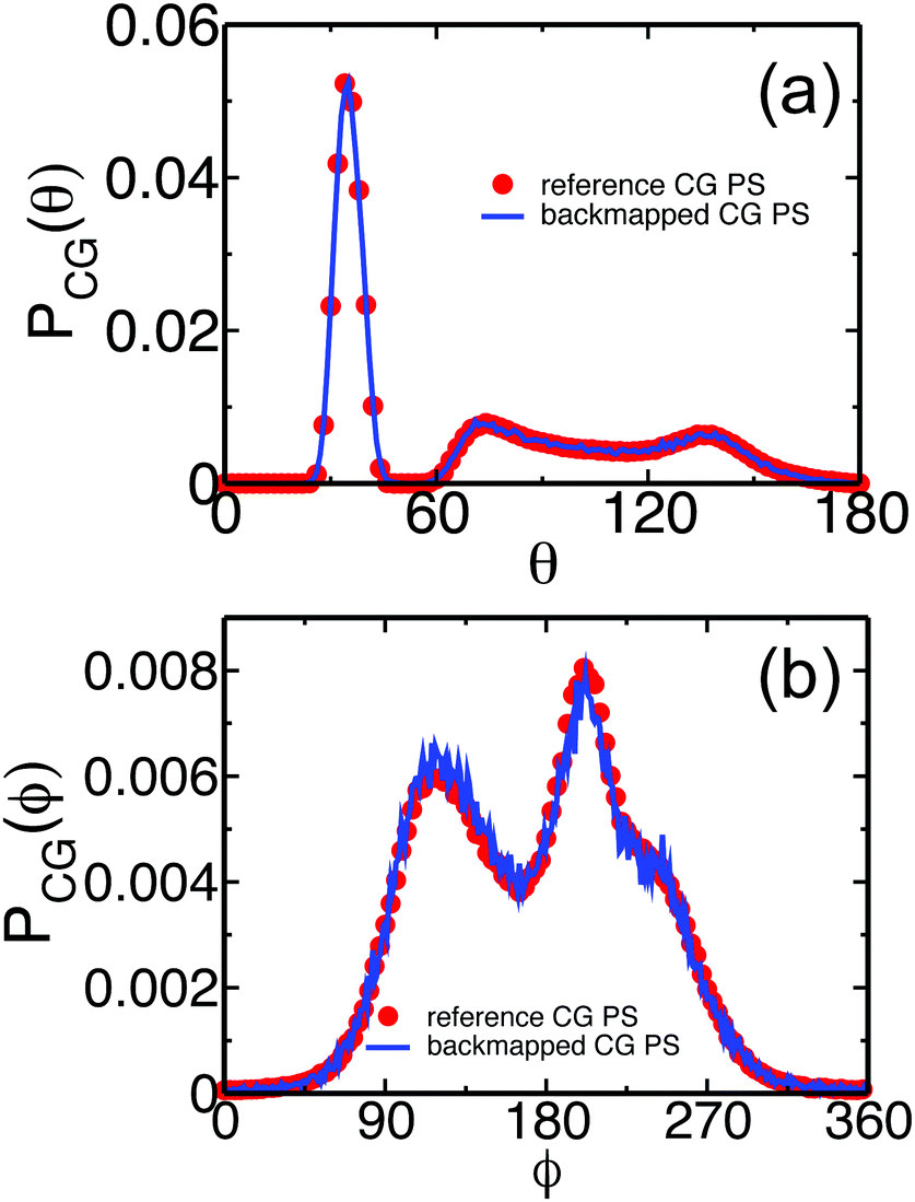 | ||
| Fig. 5 Comparison of probability distributions of (a) bond angles, PCG(θ), and (b) torsional angles, PCG(ϕ), calculated for the backmapped (lines) and ref. 14 and 53 (symbols) CG melts of PS. | ||
The structure of the polymer liquid is quantified in Fig. 6(a) and (b), presenting the total, gCG(r), and the interchain, ginter,CG(r), pair-distribution functions of superatoms in the backmapped (lines) and reference (symbols) samples. The plots obtained for backmapped and reference systems are indistinguishable from each other. The agreement between ginter,CG(r) is particularly important; thanks to the correlation-hole effect18 this quantity is a sensitive quantifier of the mesoscopic liquid structure on length scales comparable to the average size of the entire chain. The characteristic size of the correlation hole, defined by the average radius of gyration of the chains, is marked in Fig. 6(b) by the arrow. To illustrate more clearly that the backmapped melts reproduce correctly the long-wavelength density fluctuations of PS, we compare in Fig. 6(c) their static structure factor S(q) (line) with its counterpart (symbols) for reference samples. The two plots agree with each other within the statistical noise of the data. The latter is quantified via the error bars, corresponding to the standard deviation calculated from four independent backmapped CG melts of PS. From the data in Fig. 6, we obtain the isothermal compressibility, κT, of atactic polystyrene at 463 K: κT = S(q → 0)/ρkBT ≈ 8.7 × 10⁻¹⁰ Pa−1. Here ρ denotes the number density of superatoms in the CG PS configurations. The κT characterising the backmapped samples is remarkably close to κT = 8.4 × 10⁻¹⁰ Pa−1 that has been experimentally reported for PS at 473 K.70
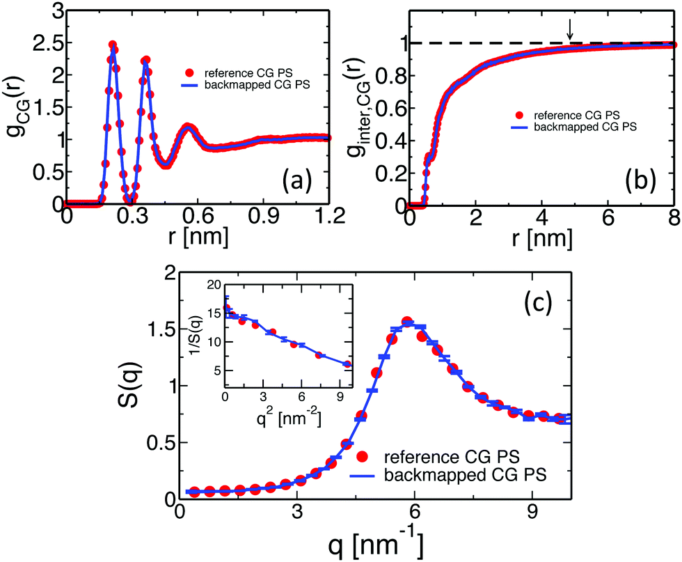 | ||
| Fig. 6 Comparison of (a) total, gCG(r), and (b) intermolecular, ginter,CG(r), pair-distribution functions calculated for the backmapped (lines) and ref. 14 (symbols) CG melts of PS. Panel (c) shows the structure factor of density fluctuations in the backmapped (lines) and reference (symbols) melts. The inset presents the behavior of 1/S(q) for q → 0, used to extract the isothermal compressibility. | ||
One of the most stringent tests of equilibration is performed in Fig. 7, where we present the internal distance plot RCG2(l)/l calculated for the backmapped (line) and reference (symbols) CG PS melts. The error-bars correspond to the 95% confidence interval and, for clarity, are shown only for the plot obtained from the backmapped melts. The error-bars grow at the tail of the plot due to fewer data available for calculating RCG2(l)/l. Within the noise of the data, the two plots match each other well and confirm the equilibration of the PS melts.
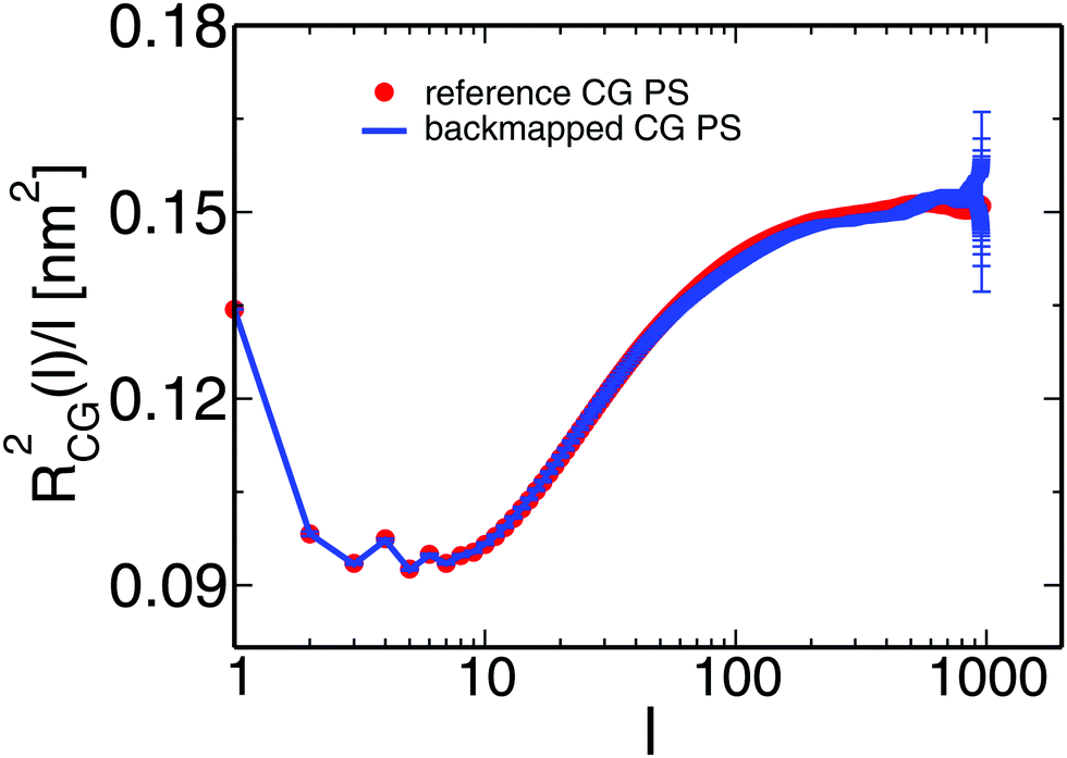 | ||
| Fig. 7 The line and the symbols present, respectively, the internal distance plots calculated for backmapped and ref. 14 CG melts of PS. | ||
3.4 Backmapping from the chemically specific coarse-grained model to the atomistic model
In the following we describe the methodology for the backmapping from the moderately (chemically specific) CG scale to the atomistic one. Note that several different methods for re-introducing atomistic detail to CG polymer chain conformations have appeared in the literature.13,17,21,53,71,72Here, inspired by the above works, we propose a generic approach that is based on “lego-like” construction of consecutive monomers along a macromolecular chain. The backmapping algorithm is presented below.
Development of a CG “lego”-particle database: given a specific CG mapping scheme for PS chains, atomistic information about each CG particle is required. To obtain such information atomistic configurations of short PS chains are analysed. More specifically, a particle database (a set of “lego” classes), based on the chosen CG mapping scheme, is constructed including two types of information: first, each type of class represents a CG particle type and holds the atoms that define it, along with their relative positions, their masses and their contributing weights on the CG particle. In the specific CG PS model two different CG types are defined: one that describes the CG bead type “A” and one for the CG bead type “B”. The constructed A and B “legos” that correspond to the specific CG PS model are shown in Fig. 8(a). Note that lego A consists of a CH2 and two half CH groups, whereas lego B consists of the phenyl ring (five CH and one C groups).
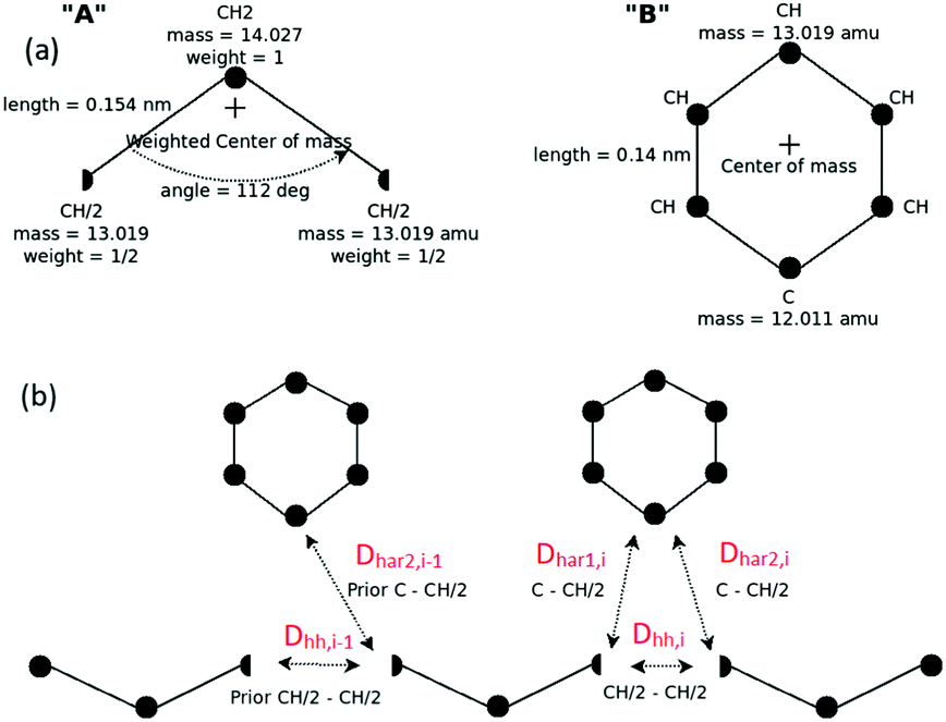 | ||
| Fig. 8 (a) “Legos” that correspond to “A” and “B” CG groups. (b) Geometric re-introduction of the atomistic detail of two consecutive PS monomers along the CG PS configurations. | ||
Second, from the analysis of the atomistic configurations, additional information is gathered about: (a) the average and the distribution of distances between two consecutive CG particles (“AB” and “BA” CG bonds) and (b) the average and the distribution of angles between three consecutive CG particles (“ABA” and “BAB” CG angles).
Re-introduction of atomistic detail using a geometric algorithm: in the next stage, given the CG PS configurations obtained from the backmapping of the blob-based to the chemically specific CG representation, the atomistic ones are created. This is achieved via a geometric algorithm, by putting each “lego” piece at the given center-of-mass of its corresponding CG particle in a consecutive way. To avoid high overlaps the “legos” are rotated around their center-of-masses, to minimise distances between neighboring atoms; see Fig. 8(b).
In more detail, for a specific PS monomer i we define Dhh,i as the distance between the two CH halves, which correspond to the same CH united-atom group, and Dhar1,i and Dhar2,i the distances between the two halves and the “C” carbon of the aromatic ring, in the ith monomer.
In addition we define θA,i = [θA,x,i, θA,y,i, θA,z,i] and θB,i = [θB,x,i, θB,y,i, θB,z,i] as the three (Eulerian) rotation angles of the A and B CG particle-“lego” of the ith monomer, respectively. Based on the above we propose, along two consecutive PS monomers, the following minimisation problem:
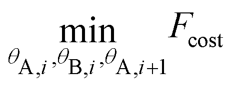 | (8) |
| Fcost = Dhh,i2 + w1((Dhar1,i − Dhar)2 + (Dhar2,i − Dhar)2) + w2(Dhh,i−12 + (Dhar2,i−1 − Dhar)2) | (9) |
The above procedure is repeated for all pairs of consecutive monomers along the PS chain, in order to obtain a first realistic PS atomistic configuration.
Energy minimisation: the re-insertion of the atomistic detail on the CG PS configurations has been extensively tested and no strong overlaps between neighboring atoms were observed. However, due to possible correlations among the CG intramolecular (bonds, angles, and dihedrals) degrees of freedom, as well as due to the fact that the geometric method does not involve thermal fluctuations, overlaps between atoms cannot be fully avoided. To treat such overlaps, in the third stage an energy minimisation procedure for all atoms is required.
We perform such a “global”, with respect to the number of atoms that are involved, minimisation scheme in two steps: first, the non-bonded interaction potential, between all UA groups, is switched off and the bonded (involving all atomistic bonds, angles and dihedrals) potential is minimised through a steepest descent method, while the centers-of-mass corresponding to the CG beads A and B are restrained in their original positions. The improper dihedral potentials used to describe the tacticity of each polymer chain by fixing the tetrahedral configuration around the sp3-C connected to the phenyl ring are also involved in the minimisation scheme. Second, the non-bonded potential is switched on the restraints on center-of-masses are removed, and the full atomistic force field (all bonded and non-bonded interactions) is minimised via a conjugate gradient algorithm.
Short MD runs: finally, in order to relax remaining stresses in the systems and to obtain a realistic atomistic trajectory at the appropriate temperature, a short NVT MD run, of about 100 ps, is executed.
Therefore, in order to validate the backmapping procedure we decide to use a low MW (1 kDa, 10mer) PS melt, at T = 463 K. First, we perform long atomistic MD simulations of atactic 10mer PS melts, using the model described in Section 2. These simulations are performed in the NPT ensemble, whereas tail corrections for the energy and pressure were applied. The integration time step was 1 fs, whereas the overall atomistic simulation time of the production runs was 100 ns.
Second, we apply the backmapping methodology, described in the previous section, to a CG 10mer PS system.14 Thus, we obtain atomistic configurations of 10mer PS without performing atomistic MD simulations.
Overall, for the low MW PS melt atomistic data are gathered both from long atomistic MD simulations (“reference” data) and from CG systems after employing the CG-to-atomistic backmapping procedure. As a direct “intramolecular” check of the backmapping process we examine the internal distance plot, analysed at the united-atom level, of a typical short-chain system (MW = 1 kDa), obtained both from long atomistic MD simulations and after backmapping of the CG configurations. This internal distance plot is defined setting in eqn (5)R2(s) ≡ RAT2(n) and m ≡ n, where RAT2(n) is the average mean square distance between two carbon atoms of the atomistic PS chains. Accordingly, n is the number of carbon atoms in the chain backbone between these two atoms. Data are shown in Fig. 9. As we can see the agreement between the two sets of data is excellent for all internal distances. Note that a similar agreement has been found before for short PS chains following a different back mapping approach.73
 | ||
| Fig. 9 Internal distance distribution, analysed at the united-atom level, of a typical system (MW = 1 kDa), obtained from long atomistic MD simulations and after backmapping of the CG configurations. | ||
The short chain PS atomistic configurations obtained from the CG ones through the backmapping procedure can be further examined by calculating the atomistic pair distribution functions, gAT(r), and comparing them against the data derived directly from the long atomistic runs. Results are presented in Fig. 10(a) and (b). First, in Fig. 10(a) data for the intramolecular distribution function, gintra,AT(r), are shown. The agreement between the two curves is excellent for all length scales, providing thus direct evidence of the applicability of the coarse-grained model to preserve the long length internal chain structure. Note that these data include all intramolecular correlations, in contrast to the internal distance distribution data shown in Fig. 9, where only correlations along the backbone atoms are considered. Thus the agreement between the two sets of data shown in Fig. 10(a) proves the ability of the backmapping methodology to reproduce the full intramolecular structure.
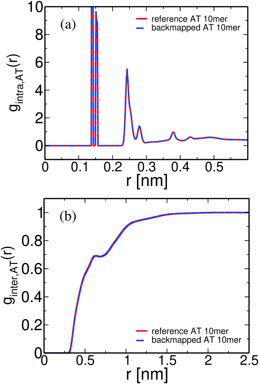 | ||
| Fig. 10 (a) Intramolecular and (b) intermolecular pair distribution functions for a PS melt (MW = 1 kDa, T = 463 K), obtained from long atomistic MD simulations, and after backmapping of the CG configurations. | ||
The intermolecular pair distribution function, ginter,AT(r), is shown in Fig. 10(b). The excellent agreement between the two different sets of data clearly demonstrates that the local packing in the backmapped atactic PS melts is also well reproduced. Note that the agreement between the intermolecular distribution functions based on different correlations, e.g. of “CH2–CH2” and of “phenyl–phenyl” groups (data not shown here) is of similar quality.
A typical well-equilibrated atomistic configuration (snapshot) of a 50 kDa PS melt with 100 chains is shown in Fig. 11.
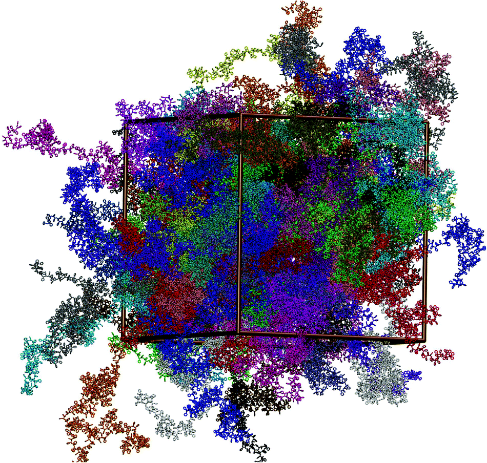 | ||
| Fig. 11 Equilibrated atomistic configuration of a 50 kDa (480mer) PS melt with 100 chains (T = 463 K). Chains are shown unwrapped (with the center-of-mass of each chain in the simulation box) and with different colors for clarity. | ||
The structure of polymeric chains, and its dependence on the molecular weight, is of special importance. Thus, in the following we compare the pair distribution functions of the long (entangled) PS chains with the data from the short (oligomeric) PS discussed above. The structure of the derived atomistic PS 480mer configuration is examined in Fig. 12(a) and (b). In Fig. 12(a) data for the atomistic intramolecular distribution function, gintra,AT(r) of both low (10mer) and high (480mer) molecular weight PS melts are shown. The agreement between the two curves at very short distances of about 0.5 nm is expected. Indeed, correlations on such length scales involve neighboring atoms along the polymer chain (i.e. atoms belonging only to one or two consecutive monomers), thus being very similar for the low and high molecular weight chains. At greater distances intramolecular distribution functions approach zero, as expected; however, gintra,AT(r) for 480mer PS chains is extended to much longer lengths.
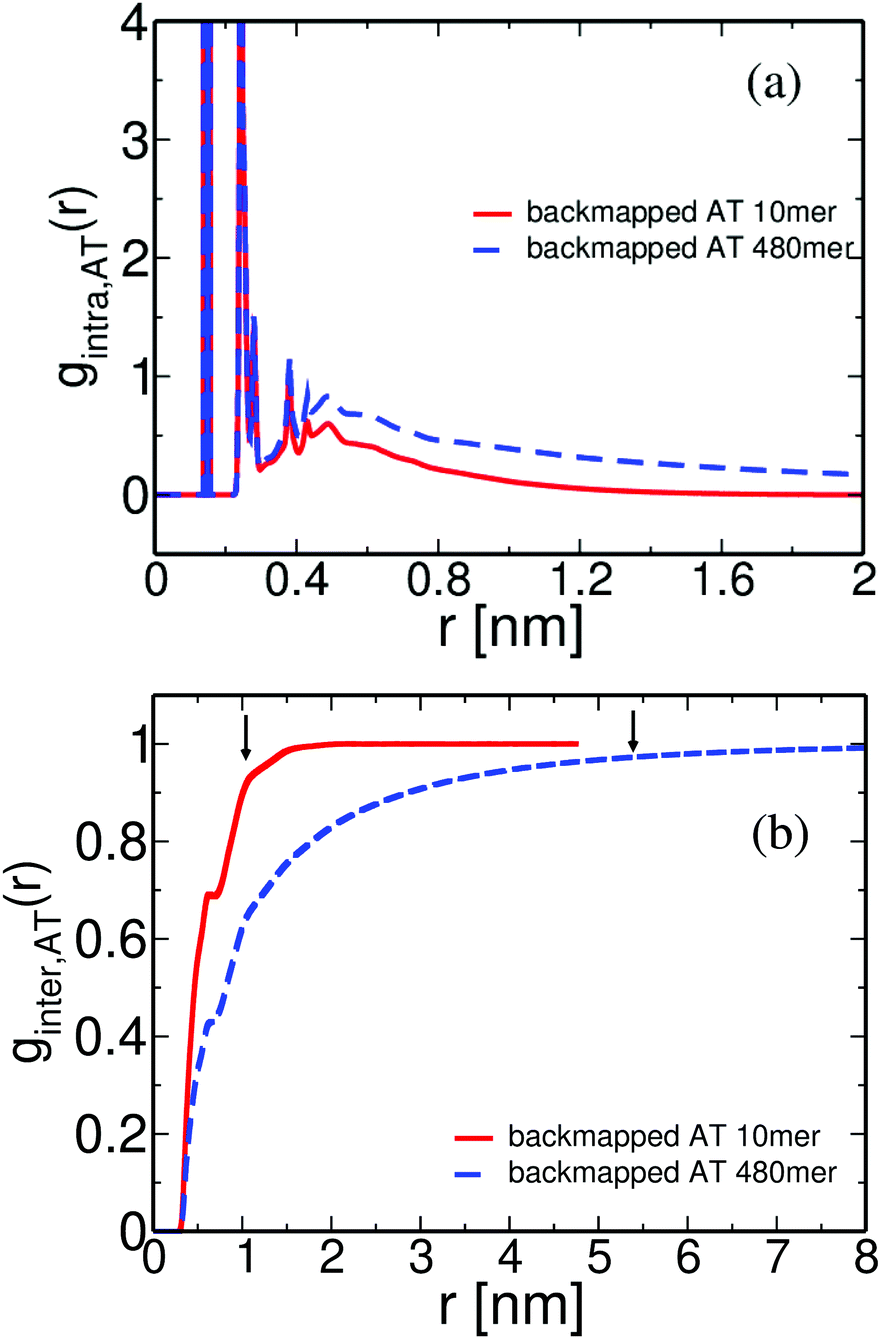 | ||
| Fig. 12 (a) Intramolecular and (b) intermolecular pair distribution functions for different PS melts, obtained directly from backmapping of the CG configurations. Arrows denote the average radius of gyration of the chains for both systems, Rg(1 kDa) = 0.9 nm and Rg(50 kDa) = 5.4 nm. | ||
Different is the case for the overall chain packing, which is directly related to the correlation hole of the polymer chains.18 Data about the intermolecular pair distribution function, ginter,AT(r), are shown in Fig. 12(b). It is obvious that the correlation hole extends over a distance of the order of the average radius of gyration of the chains; the latter is shown, for both systems, in Fig. 12(b) with arrows. In addition, for the high molecular weight chains the correlation hole becomes less deep, as has been also discussed before.49
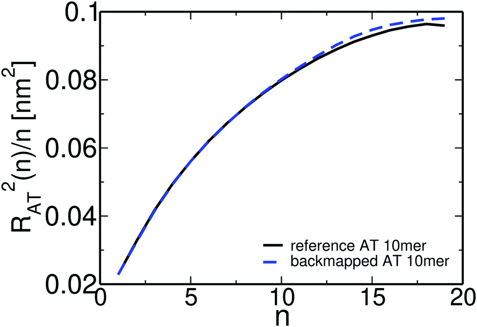
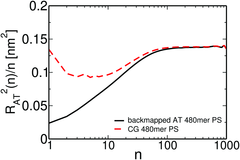
We present in Fig. 13 the internal distance plot RAT2(n)/n calculated for one representative backmapped sample of an atomistic 50 kDa PS melt (solid black line). RAT2(n) stands for the average mean square distance between n consecutive backbone carbon atoms of the atomistic PS chains. For comparison, the internal distance plot calculated for the sample of the moderately CG melt used to backmap this atomistic sample is also shown (dashed red line). For the atomistic sample, the internal distances start from a small value and then smoothly reach a plateau for n around 80–100, which corresponds to 40–50 PS monomers. This behavior at small n differs from the internal distance plot in the moderately CG representation, where RAT2(n)/n appears non-monotonous and more structured. Such differences are expected because of the averaging of the monomeric degrees of freedom performed in the CG groups. In contrast, the two plots match each other at large n, demonstrating that our “CG-to-atomistic” backmapping procedure conserves the global conformational properties that have already been equilibrated during the “blob-to-CG” backmapping stage.
 | ||
| Fig. 13 Internal distance distribution, analysed at the united-atom level, of a high MW PS chain obtained directly after backmapping of the CG configurations,without performing long atomistic MD runs. | ||
4 Conclusions and outlook
In this work, we propose a method for efficiently generating well-equilibrated configurations of high molecular-weight polymer melts, described with chemically-specific atomistic models. The method is build on a hierarchy of models, which describe the same material with different resolutions: from mesoscopic to atomistic. The modelling hierarchy includes a soft blob-based, a moderately coarse-grained, and an atomistic model. If required, more soft blob-based models can be incorporated to accelerate equilibration of larger scales. Each model in the hierarchy is parameterised to reproduce key conformational and structural properties characterising the melt, when described with the next finer-resolution model. First, the melt is efficiently equilibrated using the soft blob-based model. The details of the next level are reinserted, the system is re-equilibrated, and we proceed to the next reinsertion step. During each step of backmapping only local re-equilibration is required. Therefore, the computation time is independent of the molecular weight of the polymer that is considered.The hierarchical backmapping method presented in this study aims to deliver well-equilibrated atomistically-resolved configurations of highly entangled polymer melts. Preparing such configurations via hierarchical backmapping circumvents the major bottleneck of equilibration schemes with realistic dynamics – the need to address time-scales larger than the reptation time, τrep; i.e. the problem of long relaxation times. The backmapped atomistic configurations derived here are conceived to serve as an input for further computational studies of structural, dynamical and rheological properties, in and out of equilibrium. For the latter, the input configurations must be subjected to techniques such as standard non-equilibrium molecular dynamics (NEMD) and protracted computational times cannot be avoided. We emphasize, however, that many properties and phenomena relevant for polymer dynamics and rheology can be captured either from equilibrium MD simulations, e.g. using Green–Kubo relations for linear transport coefficients, or from NEMD simulations on time scales shorter than τrep; in either case, nevertheless, equilibrated starting states are required. Such simulations can be costly computationally but already manageable with modern super-computers.51,74–79
Finally, we mention that considering flow effects already on the level of blob-based models offers an interesting possibility. The blob-based model of our study cannot be used for a mesoscopic description of flow since it does not include a way to avoid crossings between polymer chains, which are allowed by the soft potentials. Methods for recovering non-crossability of chains in blob-based models are available, e.g. using phenomenological interactions (e.g. via slip-links80,81 or slip-springs82–85) or algorithmic detection and prevention of intersections.15,36 Performing backmapping from such “rheologically-consistent” blob-based models is an interesting perspective for generating off-equilibrium all-atom configurations.
Overall, here, as a proof-of-concept, we use the proposed multi-resolution method to equilibrate atomistically-resolved samples of melts of long atactic polystyrene chains. The preparation of such systems using brute force MD simulations is unfeasible, even with modern supercomputers. We emphasise that the method is not restricted to polystyrene and can be straightforwardly applied to equilibrate melts of other polymeric materials, where moderately CG models exist.16,86–90
Conflicts of interest
There are no conflicts to declare.Appendix: “push-off” procedure for backmapping the blob-based model to the chemically specific coarse-grained model
The whole “push-off” procedure is accomplished in 100 cycles of a molecular dynamics simulation, where each cycle is comprised of 2 × 10⁴ steps, and time step Δt = 0.0001τ (τ is the time unit in the CG PS model). (a) For all particle pairs ij other than the intramolecular (1,5) pairs rc(n) is linearly decreased from 0.9 rcutoffij (rcutoffij is the cutoff of the LJ-like potential between i and j particles) to 0.5 rcutoffij within the first 80 cycles, after which particle overlaps for those pairs can be successfully removed. (b) For the intramolecular (1,5) pairs, the corresponding force-capped radius, rc(1,5), is allowed to fluctuate (instead of decreasing linearly as in case (a)) to prevent large distortions of chain conformations. For this purpose, after each cycle, we quantify via I (see eqn (7) in Section 3.1) the deviation of the internal distance plot from the reference one. Before starting the next cycle we decrease (or increase) rc(1,5) by 0.01σ1–5 if the calculated I is negative (or positive). In this way, rc(1,5) can fluctuate within the first 80 simulation cycles. In the last 20 cycles it is reduced linearly to 0.5 rcutoff(1,5).Acknowledgements
The computing time granted by the John von Neumann Institute for Computing (NIC) on the supercomputer JURECA at Jülich Supercomputing Centre (JSC) is gratefully acknowledged. This work has been supported by the European Research Council (ERC) under the Seventh Framework Programme (FP7/2007–2013)/ERC Grant Agreement No. 340906-MOLPROCOMP. G. Zhang acknowledges the support from the National Natural Science Foundation of China (21873023). Open Access funding provided by the Max Planck Society.References
- A. Yu. Grosberg and A. R. Kokhlov, Statistical Physics of Macromolecules, AIP, New York, 1994 Search PubMed.
- M. Müller, J. Stat. Phys., 2011, 145, 967–1016 CrossRef.
- J. Zhang, D. Mukherji and K. Ch. Daoulas, Eur. Phys. J.: Spec. Top., 2016, 225, 1423–1440 CAS.
- R. Everaers, S. K. Sukumaran, G. S. Grest, C. Svaneborg, A. Sivasubramanian and K. Kremer, Science, 2004, 303, 823–826 CrossRef CAS PubMed.
- Physical Properties of Polymers Handbook, ed. J. E. Mark, Springer, 2007 Search PubMed.
- M. Doi and S. F. Edwards, The Theory of Polymer Dynamics, Oxford University Press, Oxford, 1986 Search PubMed.
- T. Spyriouni, C. Tzoumanekas and D. N. Theodorou, Macromolecules, 2007, 40, 3876–3885 CrossRef CAS.
- V. G. Mavrantzas, T. D. Boone, E. Zervopoulou and D. N. Theodorou, Macromolecules, 1999, 32, 5072–5096 CrossRef CAS.
- K. Kremer and F. Müller-Plathe, Mol. Simul., 2002, 28, 729–750 CrossRef CAS.
- W. G. Noid, J. W. Chu, G. S. Ayton, V. Krishna, S. Izvekov, G. A. Voth, A. Das and H. C. Andersen, J. Chem. Phys., 2008, 128, 244114 CrossRef CAS PubMed.
- Coarse-Graining of Condensed Phase and Biomolecular Systems, ed. G. A. Voth, CRC Press, Boca Raton, 2009 Search PubMed.
- W. G. Noid, J. Chem. Phys., 2013, 139, 090901 CrossRef CAS PubMed.
- C. Peter and K. Kremer, Soft Matter, 2009, 5, 4357–4366 RSC.
- V. A. Harmandaris, D. Reith and N. F. A. van der Vegt, Macromol. Chem. Phys., 2007, 208, 2109–2120 CrossRef CAS.
- J. T. Padding and W. J. Briels, J. Phys.: Condens. Matter, 2011, 23, 233101 CrossRef CAS PubMed.
- W. Tschöp, K. Kremer, J. Batoulis, T. Bürger and O. Hahn, Acta Polym., 1998, 49, 61–74 CrossRef.
- W. Tschöp, K. Kremer, O. Hahn, J. Batoulis and T. Bürger, Acta Polym., 1998, 49, 75–79 CrossRef.
- P. G. de Gennes, Scaling Concepts in Polymer Physics, Cornell University Press, Ithaca, New York, 1979 Search PubMed.
- R. Auhl, R. Everaers, G. S. Grest, K. Kremer and S. J. Plimpton, J. Chem. Phys., 2003, 119, 12718–12728 CrossRef CAS.
- L. A. Moreira, G. J. Zhang, F. Müller, T. Stuehn and K. Kremer, Macromol. Theory Simul., 2015, 24, 419–431 CrossRef CAS.
- P. Carbone, H. A. Karimi-Varzaneh and F. Müller-Plathe, Faraday Discuss., 2010, 144, 25–42 RSC.
- Y. R. Sliozberg, M. Kröger and T. L. Chantawansri, J. Chem. Phys., 2016, 144, 154901 CrossRef PubMed.
- J. P. Wittmer, P. Beckrich, H. Meyer, A. Cavallo, A. Johner and J. Baschnagel, Phys. Rev. E: Stat., Nonlinear, Soft Matter Phys., 2007, 76, 011803 CrossRef CAS PubMed.
- J. Glaser, J. Qin, P. Medapuram and D. C. Morse, Macromolecules, 2014, 47, 851–869 CrossRef CAS.
- H. Meyer, E. Horwath and P. Virnau, ACS Macro Lett., 2018, 7, 757–761 CrossRef CAS.
- B. Steinmüller, M. Müller, K. R. Hambrecht, G. D. Smith and D. Bedrov, Macromolecules, 2011, 45, 1107–1117 CrossRef.
- G. J. Zhang, L. A. Moreira, T. Stuehn, K. Ch. Daoulas and K. Kremer, ACS Macro Lett., 2014, 3, 198–203 CrossRef CAS.
- D. Ozog, J. McCarty, G. Gossett, A. D. Malony and M. Guenza, J. Comput. Sci., 2015, 9, 33–38 CrossRef.
- C. Svaneborg, H. A. Karimi-Varzaneh, N. Hojdis, F. Fleck and R. Everaers, Phys. Rev. E, 2016, 94, 032502 CrossRef PubMed.
- A. J. Parker and J. Rottler, Macromol. Theory Simul., 2014, 23, 401–409 CrossRef CAS.
- V. Sethuraman, S. Mogurampelly and V. Ganesan, Macromolecules, 2017, 50, 4542–4554 CrossRef CAS.
- M. Laso, H. C. Öttinger and U. W. Suter, J. Chem. Phys., 1991, 95, 2178–2182 CrossRef CAS.
- M. Murat and K. Kremer, J. Chem. Phys., 1998, 108, 4340–4348 CrossRef CAS.
- C. Likos, Phys. Rep., 2001, 348, 267–439 CrossRef CAS.
- P. G. Bolhuis, A. A. Louis, J. P. Hansen and E. J. Meijer, J. Chem. Phys., 2001, 114, 4296–4311 CrossRef CAS.
- J. T. Padding and W. J. Briels, J. Chem. Phys., 2001, 115, 2846–2859 CrossRef CAS.
- F. Eurich and P. Maass, J. Chem. Phys., 2001, 114, 7655–7668 CrossRef CAS.
- V. Krakoviack, J.-P. Hansen and A. A. Louis, Phys. Rev. E: Stat., Nonlinear, Soft Matter Phys., 2003, 67, 041801 CrossRef CAS PubMed.
- T. Vettorel, G. Besold and K. Kremer, Soft Matter, 2010, 6, 2282–2292 RSC.
- A. J. Clark, J. McCarty, I. Y. Lyubimov and M. G. Guenza, Phys. Rev. Lett., 2012, 109, 168301 CrossRef CAS PubMed.
- R. Menichetti1 and A. Pelissetto, J. Chem. Phys., 2013, 138, 124902 CrossRef PubMed.
- G. D'Adamo, A. Pelissetto and C. Pierleoni, J. Chem. Phys., 2013, 138, 234107 CrossRef PubMed.
- G. J. Zhang, K. Ch. Daoulas and K. Kremer, Macromol. Chem. Phys., 2013, 214, 214–224 CrossRef CAS.
- A. Narros, C. N. Likos, A. J. Moreno and B. Capone, Soft Matter, 2014, 10, 9601–9614 RSC.
- G. D'Adamo, R. Menichetti, A. Pelissetto and C. Pierleoni, Eur. Phys. J.: Spec. Top., 2015, 224, 2239–2267 Search PubMed.
- D. Yang and Q. Wang, J. Chem. Phys., 2015, 142, 054905 CrossRef.
- G. J. Zhang, T. Stuehn, K. Ch. Daoulas and K. Kremer, J. Chem. Phys., 2015, 142, 221102 CrossRef PubMed.
- T. Ohkuma, K. Kremer and K. Daoulas, J. Phys.: Condens. Matter, 2018, 30, 174001 CrossRef PubMed.
- V. A. Harmandaris and K. Kremer, Macromolecules, 2009, 42, 791–802 CrossRef CAS.
- V. A. Harmandaris and K. Kremer, Soft Matter, 2009, 5, 3920–3926 RSC.
- C. Baig and V. A. Harmandaris, Macromolecules, 2010, 43, 3156–3160 CrossRef CAS.
- C. D. Wick, M. G. Martin and J. I. Siepmann, J. Phys. Chem. B, 2000, 104, 8008–8016 CrossRef CAS.
- V. A. Harmandaris, N. Adhikari, N. F. A. van der Vegt and K. Kremer, Macromolecules, 2006, 39, 6708–6719 CrossRef CAS.
- C. Liu, K. Kremer and T. Bereau, Adv. Theory Simul., 2018, 1, 1800024 CrossRef.
- P. J. Flory, J. Chem. Phys., 1949, 17, 303–310 CrossRef CAS.
- D. Lhuillier, J. Phys., 1988, 49, 705–710 CrossRef CAS.
- In previous implementations of the soft sphere model the prefactor Nb was adsorbed into c2. Here it appears explicitly in the term c2Nb2/σ3 (see eqn (2)) to highlight the relevance to the Flory free energy.
- In previous implementations of the soft sphere model the prefactor Nb2 was adsorbed into ε.
- R. L. C. Akkermans and W. J. Briels, J. Chem. Phys., 2001, 114, 1020–1031 CrossRef CAS.
- Q. Wang and D. Yang, Polymer, 2017, 111, 103–106 CrossRef CAS.
- M. Dinpajooh and M. G. Guenza, Polymer, 2017, 117, 282–286 CrossRef CAS.
- G. Fleisher, Colloid Polym. Sci., 1987, 265, 89–95 CrossRef.
- M. Antonietti, K. J. Fölsch and H. Sillescu, Makromol. Chem., 1987, 188, 2317–2324 CrossRef CAS.
- L. J. Fetters, D. L. Lohse, D. Richter, T. A. Witten and A. Zirkel, Macromolecules, 1994, 27, 4639–4647 CrossRef CAS.
- A. P. Lyubartsev and A. Laaksonen, Phys. Rev. E: Stat. Phys., Plasmas, Fluids, Relat. Interdiscip. Top., 1995, 52, 3730–3737 CrossRef CAS.
- F. Müller-Plathe, ChemPhysChem, 2002, 3, 754–769 CrossRef.
- H.-P. Hsu and K. Kremer, J. Chem. Phys., 2016, 144, 154907 CrossRef PubMed.
- J. D. Halverson, T. Brandes, O. Lenz, A. Arnold, S. Bevc, V. Starchenko, K. Kremer, T. Stuehn and D. Reith, Comput. Phys. Commun., 2013, 184, 1129–1149 CrossRef CAS.
- R. S. Graham, A. E. Likhtman and T. C. B. McLeish, J. Rheol., 2003, 47, 1171–1200 CrossRef CAS.
- J. E. Mark, Physical Properties of Polymers Handbook, Springer, 2nd edn, 2007 Search PubMed.
- L. E. Lombardi, M. A. Martí and L. Capece, Bioinformatics, 2016, 32, 1235–1237 CrossRef CAS PubMed.
- G. Santangelo, A. Di Matteo, F. Müller-Plathe and G. Milano, J. Phys. Chem. B, 2007, 111, 2765–2773 CrossRef CAS PubMed.
- D. Fritz, V. A. Harmandaris, K. Kremer and N. F. A. van der Veg, Macromolecules, 2009, 42, 7579–7588 CrossRef CAS.
- J. Ramos, J. F. Vega, D. N. Theodorou and J. Martinez-Salazar, Macromolecules, 2008, 41, 2959–2962 CrossRef CAS.
- J.-X. Hou, C. Svaneborg, R. Everaers and G. S. Grest, Phys. Rev. Lett., 2010, 105, 068301 CrossRef PubMed.
- H. P. Hsu and K. Kremer, ACS Macro Lett., 2018, 7, 107–111 CrossRef CAS PubMed.
- H. P. Hsu and K. Kremer, Phys. Rev. Lett., 2018, 121, 167801 CrossRef PubMed.
- S. Jeong, J. M. Kim and C. Baig, Macromolecules, 2017, 50, 3424–3429 CrossRef CAS.
- M. Kröger and S. Hess, Phys. Rev. Lett., 2000, 85, 1128–1131 CrossRef.
- A. E. Likhtman, Macromolecules, 2005, 38, 6128–6139 CrossRef CAS.
- D. M. Nair and J. D. Schieber, Macromolecules, 2006, 39, 3386–3397 CrossRef CAS.
- Y. Masubuchi, J. I. Takimoto, K. Koyama, G. Ianniruberto, G. Marrucci and F. Greco, J. Chem. Phys., 2001, 115, 4387–4394 CrossRef CAS.
- J. Oberdisse, G. Ianniruberto, F. Greco and G. Marrucci, Rheol. Acta, 2006, 46, 95–109 CrossRef.
- Y. Masubuchi, T. Uneyama, H. Wanatabe, G. Ianniruberto, F. Greco and G. Marrucci, J. Chem. Phys., 2010, 132, 134902 CrossRef PubMed.
- V. Chappa, D. Morse, A. Zippelius and M. Müller, Phys. Rev. Lett., 2012, 109, 148302 CrossRef PubMed.
- B. Hess, S. León, N. F. A. van der Vegt and K. Kremer, Soft Matter, 2006, 2, 409–414 RSC.
- T. Ohkuma and K. Kremer, Polymer, 2017, 130, 88–101 CrossRef CAS.
- Y. N. Pandey, A. Brayton, C. Burkhart, G. J. Papakonstantopoulos and M. Doxastakis, J. Chem. Phys., 2014, 140, 054908 CrossRef PubMed.
- Q. Sun and R. Faller, J. Chem. Phys., 2007, 126, 144908 CrossRef PubMed.
- C. A. Lemarchand, M. Couty and B. Rousseau, J. Chem. Phys., 2017, 146, 074904 CrossRef PubMed.
| This journal is © The Royal Society of Chemistry 2019 |