
 Open Access Article
 This Open Access Article is licensed under a Creative Commons Attribution-Non Commercial 3.0 Unported Licence
Collision cross section compendium to annotate and predict multi-omic compound identities†
Jaqueline A.
Picache
 ,
Bailey S.
Rose
,
Andrzej
Balinski
,
Katrina L.
Leaptrot
,
Stacy D.
Sherrod
,
Jody C.
May
and
John A.
McLean
*
,
Bailey S.
Rose
,
Andrzej
Balinski
,
Katrina L.
Leaptrot
,
Stacy D.
Sherrod
,
Jody C.
May
and
John A.
McLean
*
Department of Chemistry, Center for Innovative Technology, Vanderbilt Institute of Chemical Biology, Vanderbilt Institute for Integrative Biosystems Research and Education, Vanderbilt-Ingram Cancer Center, Vanderbilt University, Nashville, Tennessee 37235, USA. E-mail: john.a.mclean@vanderbilt.edu
First published on 27th November 2018
Abstract
Ion mobility mass spectrometry (IM-MS) expands the analyte coverage of existing multi-omic workflows by providing an additional separation dimension as well as a parameter for characterization and identification of molecules – the collision cross section (CCS). This work presents a large, Unified CCS compendium of >3800 experimentally acquired CCS values obtained from traceable molecular standards and measured with drift tube ion mobility-mass spectrometers. An interactive visualization of this compendium along with data analytic tools have been made openly accessible. Represented in the compendium are 14 structurally-based chemical super classes, consisting of a total of 80 classes and 157 subclasses. Using this large data set, regression fitting and predictive statistics have been performed to describe mass-CCS correlations specific to each chemical ontology. These structural trends provide a rapid and effective filtering method in the traditional untargeted workflow for identification of unknown biochemical species. The utility of the approach is illustrated by an application to metabolites in human serum, quantified trends of which were used to assess the probability of an unknown compound belonging to a given class. CCS-based filtering narrowed the chemical search space by 60% while increasing the confidence in the remaining isomeric identifications from a single class, thus demonstrating the value of integrating predictive analyses into untargeted experiments to assist in identification workflows. The predictive abilities of this compendium will improve in specificity and expand to more chemical classes as additional data from the IM-MS community is contributed. Instructions for data submission to the compendium and criteria for inclusion are provided.
Introduction
Mass spectrometry (MS) has become a central technique for the investigation of the global profile of biochemical species in molecular phenomic studies.1,2 These studies aim to address the grand challenges of biomedical research including comprehensive descriptions of biological systems, natural product and drug discovery endeavors, omics sciences to improve health outcomes, and progress in synthetic biology.3–6 As the complexity of the systems being studied increases, so must the ability to increase analyte coverage. Orthogonal separation techniques such as gas and liquid chromatography are often used in conjunction with MS to improve coverage. However, feature annotation and identification from such experiments can be challenging due to analyte co-elution and retention time variability among other issues.7These challenges can be addressed with the use of additional analytical separation techniques, such as ion mobility spectrometry coupled to MS (IM-MS), which is selective to the analyte gas phase structure.3,8 One practical benefit of using gas-phase ion mobility is that there are no memory effects or sample-to-sample carryover due to the continuous replacement of the separation gas. Additionally, IM separations do not require disposable solvents or packed columns and are amenable to all ionizable chemical species. The main advantages of IM-MS are an increase in analytical peak capacity as well as the ability to measure an analyte's gas phase mobility by means of an experimental drift time.9 This mobility can then be used to calculate an analyte's collision cross section (CCS), a rotationally averaged surface area of the molecule in its ionic form. These CCS values are specific and can be compared across different laboratories making them particularly well-suited for species identification and characterization purposes. Previous studies indicate that the level of reproducibility varies across analyte classes.10,11 A recent study using drift tube IM-MS has shown that CCS values can be measured within a 0.30% RSD when data is acquired with a previously established standardized method.12
As a result of these advantages, several research groups have used IM-MS to build CCS libraries in which the measured values serve as additional molecular descriptors for assigning identities to unknown analytes. While not an exhaustive list, a few of the larger libraries to note are: Li and colleagues' peptide database which includes >2300 CCS values,13 Pagel and colleagues' glycomics database of >900 CCS values,14 and Xu and colleagues' small molecule database containing >1400 CCS values.15 Additionally, many excellent smaller CCS libraries have been generated for lipids,16–18 primary metabolites,18–20 secondary metabolites and other natural products,18,21,22 as well as illicit substances23 among others.
While each of these libraries adds to the working knowledge of the IM-MS field, there remain challenges that need to be addressed. The first is reconciling CCS measurements across various IM implementations such as drift tube (DTIMS), traveling wave (TWIMS), ion trapping (TIMS), and structures for lossless ion manipulation (SLIM) techniques. Inherently, these techniques utilize different methodologies for determining the gas-phase CCS, namely DTIMS (and drift tube-based SLIM) utilize the fundamental ion mobility relationship for correlating the measured arrival times directly to CCS, whereas the other IM techniques obtain a CCS value through calibration. In order to reconcile non-DTIMS CCS values with DTIMS values, proper calibrants must be chosen for a given experiment, which can prove challenging.10,24 An in-depth discussion of considerations for comparing CCS information obtained from different IM techniques can be found in a recent review by Gabelica et al.25
Another challenge lies in the difficulty of accurately and efficiently extracting drift time measurements from raw data files in large scale. Currently, most DTIMS drift times for chemical standards are manually extracted which improves accuracy at a cost of throughput. However, several software options exist that aim to automate the extraction of drift times on a large scale and/or predict drift times.26,27 The recent IM-MS analysis addendum to Skyline is one example that has made considerable strides in these efforts,28,29 but the IM-MS field is still working towards a streamlined analytic workflow.
Other informatics programs aim to predict CCS values based on experimental data and chemical structure. Some examples of these software include Zhu and colleague's machine learning algorithms for metabolites (MetCCS) and lipids (LipidCCS).16,19 A major barrier to the success of machine learning CCS prediction is that algorithm training sets are generally not yet large and/or specific enough.30 An alternative strategy recently described by Colby, et al. is the in silico chemical library engine (ISiCLE) workflow which utilizes a combination of molecular dynamics, quantum chemistry, and ion mobility calculations in order to predict CCS values based on theoretical structure information.31 These CCS prediction efforts are critically important for determining CCS values where empirical measurements on authentic chemical standards are unavailable.
To aid in the mainstream adoption of IM in analyte identification workflows, we explored the potential in curating libraries of empirical CCS values measured via ion mobility into a single, self-consistent compendium. The Unified CCS compendium presented herein serves as a tool where new data from the community can be vetted using a quality control protocol and subsequently integrated. Included in this curated compendium are several prevalent calibrant sets (polypeptides, branched phosphazenes, inorganic salt clusters, etc.), as well as molecular standards from a variety of chemical classes measured using DTIMS. These data sets can be used as reference values for other IM-MS techniques. Furthermore, this tool incorporates annotative features (i.e. visualization of chemical locales of molecules) and predictive statistics (chemical structure-based trends) to aid in identifying unknown biochemical species. These predictive trends serve as a powerful filter for increasing confidence in tentative identifications. In order to demonstrate the efficacy of this approach, the structural filtering method was applied to metabolites in a human serum sample. The full interactive visualization of the compendium, as well as inclusion criteria and guidelines for submitting additional CCS measurements, can be found as an open access tool.32
Experimental section
Materials and instrumentation
Methanol (MeOH), water, acetonitrile (ACN), isopropanol (IPA), and formic acid of Optima grade purity were purchased from Fisher Scientific (Fair Lawn, NJ). Anhydrous methyl-tert-butyl ether (MTBE) was purchased from Sigma Aldrich (St. Louis, MO). Normal human serum was purchased from Utak (Valencia, CA). A mixture of fluoroalkyl phosphazenes, tris(fluoroalkyl)triazines, betaine, and trifluoracetic acid reference standards were purchased from Agilent Technologies (G1969-85000, Santa Clara, CA). In this manuscript, liquid chromatography MS (LC-MS) and LC-IM-MS data were acquired using a 1290 Infinity LC system and a 6560 IM-QTOF MS (Agilent Technologies).Data sources and inclusion parameters
The primary sources of the 3833 IM-MS measurements included in the compendium are reported in a series of manuscripts found elsewere.10,12,18,33–38 In order to provide highly repeatable and reproducible data, the compendium currently only contains CCS values calculated from the fundamental low-field ion mobility equation (Mason–Schamp relationship) incorporated into a standardized inter-laboratory protocol for single field and stepped field DTIMS acquisition on a commercial uniform-field IM-MS instrument (6560, Agilent).12,39,40 In-depth information about single and stepped field DTIMS has previously been described.12 All measurements were acquired in triplicate and aligned with a suite of 13 reference standards (Agilent Technologies) containing symmetrically-branched fluoroalkyl phosphazines, namely hexaxis(fluoroalkoxy)phosphazines, tris(fluoroalkyl)triazines, betaine, and trifluoracetic acid. These reference standards were previously measured with very high precision; and it is currently believed that these CCS values are among the most accurate obtained to date.12In total, there are 1216 single field measurements within the compendium; and the average relative standard deviation (RSD) for the single field measurements is 0.12%. Compounds were matched to reference standards' values from an inter-laboratory study.12 The average percent error of compendium CCS measurements was found to be 0.04% and −0.33% for positive and negative modes, respectively, with all percent error values at ≤0.58% for both polarities. The remaining 2617 stepped field values were reconciled by calculating a “true effective length” for each data set (data set defined as a group of measurements collected in a one-day acquisition period) using calibrant measurements within the set. This “true effective length” was then used to align measurements with reference standards' values. More details and tools to calculate “true effective length” as well as instructions to calibrate acquired stepped field CCS data is found in ESI Section S3.† Once each data set was individually scaled, the average RSD for stepped field measurements was calculated to be 0.32%. When compared to inter-laboratory reference values, average percent errors were 0.07% and 0.01% for positive and negative modes, respectively. Ninety-one percent of matched values had a percent error ≤1% for both polarities. These empirically-derived metrics, in conjunction with known errors propagated in this system,12 were subsequently used as the compendium's data inclusion criteria. Full descriptions of the inclusion criteria and instructions for submitting data to the compendium can be found in ESI Section S2.†
Data preparation, statistical modeling, and visualization
Data from all sources were curated into a unified format using the statistical computing programming environment R (R Foundation for Statistical Computing, Vienna, Austria).41 This unified format includes the following information for each compendium entry: name, formula, CAS registry number (when available), mass-to-charge (m/z), charge state, ion species, size-to-charge (CCS/z), percent RSD, and number of observed DTIMS peaks. Charge-normalization of mobility measurements39via CCS/z was utilized to preserve the original drift time scale and analysis consistency.39 In drift time spectra, ions of similar mass and higher charge states typically have smaller drift times than lower charge state ions; and therefore, appear lower when visualized in drift time vs. m/z space. Contrastingly, higher charge state ions appear higher than lower charge state ions when visualized in CCS vs. m/z space. By charge-normalizing, ions appear in CCS/z vs. m/z space as they would in drift time vs. m/z space. Furthermore, when values were not charge-normalized, statistical modeling could not be standardized and was charge-state dependent. The number of DTIMS peaks observed for each molecule is included in the compendium. The number of DTIMS peaks observed for each molecule is included in the compendium. These data meet the outlined criteria and follow the standardized IM-MS data reporting efforts led by Gabelica, et al.42 Briefly, all observed DTIMS peaks are reported in the online compendium compound table via a peak number assignment where the smallest CCS/z (earliest drift time) will be assigned number 1 and subsequent peaks will be assigned 2, 3, etc. Compounds with one observed peak will be assigned a “1”. Additional information regarding DTIMS peak annotation can be found in ESI Section S1.†The unified format also includes a hierarchical chemical classification for each compound which includes a kingdom, super class, class, and subclass based on structure. This was performed via the ClassyFire web-based application which operates using a comprehensive chemical ontology (ChemOnt) that classifies each molecule based on its SMILES or InChi Key identifier as an input.43,44 For example, a phosphatidylcholine would be classified as a member of the organic compound kingdom, the lipids and lipid-like molecules super class, the glycerophospholipid class, and the glycerophosphocholine subclass.
Iterative nonlinear regression modeling was performed using the R program for each chemical class and subclass that contained at least ten data points. Source code for this statistical modeling is provided on the McLean Research Group Github.45 Each class was tested against three nonlinear regression models: a power fit (PF), a four-parameter sigmoidal fit (4P), and a five-parameter sigmoidal fit. Representative equations for these models can be found in ESI Section S5.† These models were chosen based on previous work.34,46,47 The goodness of fit for each model was assessed using the corrected Akaike information criterion (AICc) for each of the three models. This conservative metric accounts for small sample sizes, bias correction, and varying degrees of freedom in nonlinear candidate models; and has previously been shown to be highly reliable when comparing nonlinear models.48,49 The model with the lowest AICc value was taken to be the best fit. Ninety-nine percent confidence (CI) and predictive (PI) intervals were calculated as described in ESI Section S5 eqn (4) and (5),† respectively. CI and PI were calculated in the same manner for all nonlinear regressions.
The Unified CCS compendium was visualized using the following open-source R packages: plotly (v4.7.1), ggplot2 (v2.2.1.900), data.table (v1.10.4-3), plyr (v1.8.4), and shiny.50–54 Source code for the compendium GUI can be found on the McLean Research Group Github.45
Evaluation of the compendium in the analysis of human serum
Non-endogenous fatty acids 17![[thin space (1/6-em)]](https://www.rsc.org/images/entities/char_2009.gif) :0 and 19:0 were used as internal standards and added into 100 μL control human serum. 800 μL of cold MeOH (−20 °C) was subsequently added and the sample was stored at −20 °C overnight to precipitate out proteins. The sample was subsequently centrifuged at 14000 rpm and 4 °C for five minutes. The supernatant was collected; and 2.4 mL ice cold MTBE and 800 μL ice cold water were added. This MTBE:MeOH:water sample was vortexed then centrifuged at 10000 rpm and 4 °C for ten minutes. The nonpolar liquid fraction was siphoned, dried under vacuum, and stored at −20 °C until use. Dried fractions were resuspended in 100 μL of 70:18:12 water:IPA:ACN and analyzed via LC-MS and LC-IM-MS. Further details are provided in ESI Section S6.† LC-MS data was analyzed using Progenesis QI (v2.3, Nonlinear Dynamics, Durham, NC). Resulting features were tentatively identified using the Metlin Metabolomics and LipidBlast databases.55,56 LC-IM-MS raw acquisition files were converted to mzML format using MSConvert (v3.0, ProteoWizard).57 Drift time values from LC-IM-MS experiments for individual process replicates were extracted using an internally developed Python script45 in which drift times were matched against the retention time and m/z of the aforementioned tentatively identified compounds. These match functions had a threshold of 30 seconds (or 1% variation) for retention time and 5 ppm for m/z, respectively. Once drift times were extracted from the mzML data files, CCS/z values were calculated from the Mason–Schamp relationship using the averaged drift times. Chemical class probability hierarchies were analyzed using distance of the mean calculations based on where serum CCS/z values fell within the compendium as compared to the regression models.
:0 and 19:0 were used as internal standards and added into 100 μL control human serum. 800 μL of cold MeOH (−20 °C) was subsequently added and the sample was stored at −20 °C overnight to precipitate out proteins. The sample was subsequently centrifuged at 14000 rpm and 4 °C for five minutes. The supernatant was collected; and 2.4 mL ice cold MTBE and 800 μL ice cold water were added. This MTBE:MeOH:water sample was vortexed then centrifuged at 10000 rpm and 4 °C for ten minutes. The nonpolar liquid fraction was siphoned, dried under vacuum, and stored at −20 °C until use. Dried fractions were resuspended in 100 μL of 70:18:12 water:IPA:ACN and analyzed via LC-MS and LC-IM-MS. Further details are provided in ESI Section S6.† LC-MS data was analyzed using Progenesis QI (v2.3, Nonlinear Dynamics, Durham, NC). Resulting features were tentatively identified using the Metlin Metabolomics and LipidBlast databases.55,56 LC-IM-MS raw acquisition files were converted to mzML format using MSConvert (v3.0, ProteoWizard).57 Drift time values from LC-IM-MS experiments for individual process replicates were extracted using an internally developed Python script45 in which drift times were matched against the retention time and m/z of the aforementioned tentatively identified compounds. These match functions had a threshold of 30 seconds (or 1% variation) for retention time and 5 ppm for m/z, respectively. Once drift times were extracted from the mzML data files, CCS/z values were calculated from the Mason–Schamp relationship using the averaged drift times. Chemical class probability hierarchies were analyzed using distance of the mean calculations based on where serum CCS/z values fell within the compendium as compared to the regression models.
Results and discussion
CCS compendium properties
The Unified CCS compendium compiled in this work consists of a total of 3833 CCS values (see inclusion criteria in the Experimental section) obtained with uniform drift tube instruments in nitrogen drift gas utilizing a standardized CCS protocol.12 Measurements consist of 2740 cations and 1093 anions, all of which were acquired in replicates of ≥3. Associated measurement RSDs can be found on the web-based compendium.32 Thirteen ion species types are represented as indicated in Fig. 1a. The most common species observed were proton coordination (38%), proton loss (27%), and sodium coordination (25%). Ion species were assigned based on the charge source of the molecule. For example, if a compound was observed as [M + 2Na–H]+, the ion species was labelled as “+Na”. Likewise, if a compound had multiple charge carriers of the same type, such as [M + 4H]4+, it was labelled as “+H”. Compounds with multiple different equal charge carries, such as [M + H + K]2+ were recorded as both “+H” and “+K”. The charge distribution, Fig. 1b, in the compendium ranged from +1 to +31 for cations and −1 to −3 for anions. More than 90% of the compounds were singly or doubly charged. Overall, replicate measurements were highly reproducible as evaluated by RSD. The global average RSD was 0.25%; and 97% of all compounds had an RSD of <1.0%. The average RSD per CCS/z bin is shown in Fig. 1c. RSD is observed to increase as CCS/z increases due to multiple observed conformers in larger molecules. Under highly controlled interlaboratory experimental conditions, RSD is <0.3%;12 and the empirical RSD threshold of 0.7% for the compendium is a practical limit for data from independent studies. The compendium data set spans a m/z range of ca. 74 to ca. 3300 Da. However, most of the compounds are <1500 Da. The full distribution of compound masses is shown in Fig. 1d.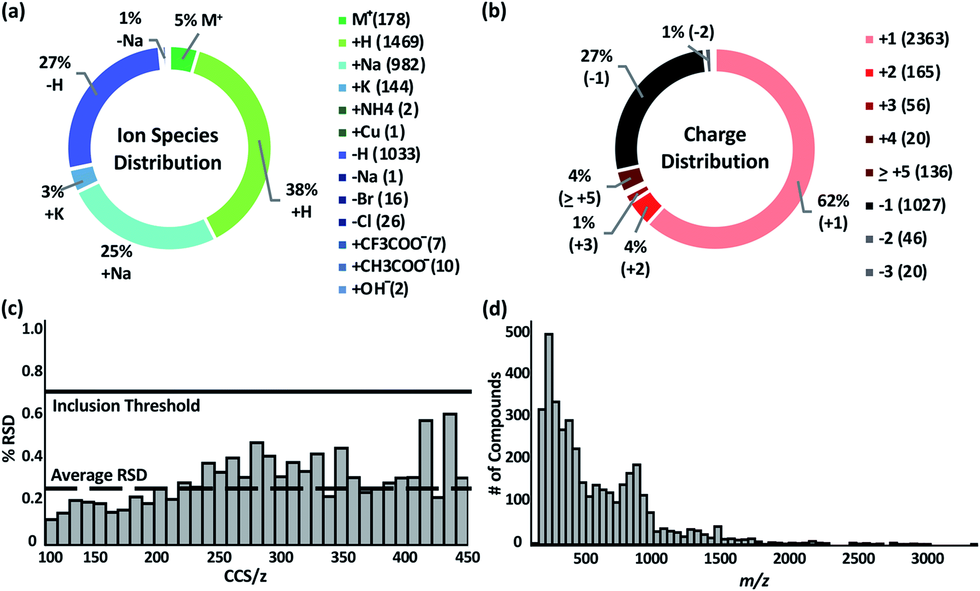 | ||
| Fig. 1 (a and b) Overall distribution of the 3833 measured ions from (+) and (−) ion polarity modes by ion species and charge state. (c) Relative standard deviation (RSD) of all measurements binned by CCS/z. Global average RSD is 0.25%, and compendium RSD threshold is 0.7%. (d) Distribution of ions contained in the database as a function of the m/z. | ||
CCS compendium visualization
The data set was visualized using code written in the R language. The graphical user interface (GUI) of the Unified CCS compendium is shown in Fig. 2a and is accessible online.32 The default view for this GUI is to show all data grouped by super class. Users have the ability to zoom and select regions of interest which facilitates maneuvering densely populated areas. By hovering the cursor over any data point, as shown in Fig. 2b, users can access specific information regarding the corresponding entry including the compound's name, molecular formula, CAS identity, m/z, observed charge species, CCS/z and associated RSD, source citation, and digital object identifier. The interactive GUI can be tailored to the user's needs. Search functionality allows users to find data on any compound within the compendium's compound table. Users can also isolate a specific data subset based on ion polarity, adduct type, super class, class, and data source. Subsetting data by super class or class reveals its CCS/z vs. m/z area of occupancy.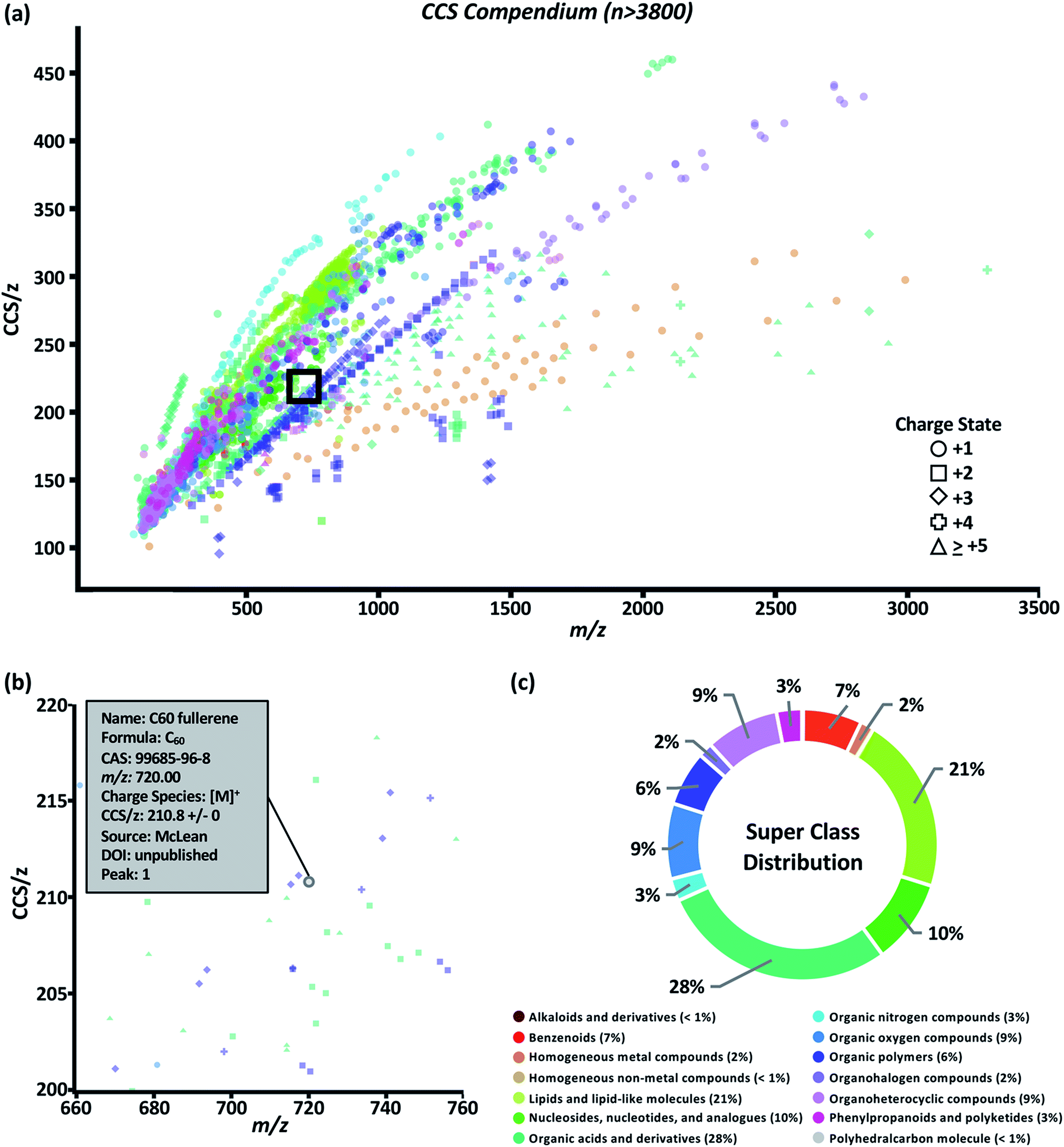 | ||
| Fig. 2 Compendium interface (a) depicting measured data points classified into super classes indicated in the legend above. An enlarged version of the area within the black box is shown in (b) to illustrate how each data point reveals an information box in the online compendium. (c) Distribution of compounds across the 14 structural super classes. | ||
The compendium covers 14 super classes which delineate into 80 classes and 157 subclasses. The distribution of compounds into each super class is summarized in Fig. 2c. A list of super classes including m/z range and number of compounds per super class is summarized in Table 1. Super classes and their subsequent classes are further described in ESI Section S4.† Full classification of individual compounds can be found on the web-based compendium.32 Of the 80 classes, 48 had a sufficient (n > 10) number of data points to undergo regression fitting tests. In total, 24 classes and 24 subclasses were modeled. As new data is added and regression fitting algorithms are iterative, it should be noted that the most up-to-date regression model equations can be found online.32 A few observations can be made from the data fitting study. Both four-parameter (ESI Section S5, eqn (2)†) and five-parameter (ESI Section S5, eqn (3)†) regressions were the best fit more frequently for classes in which m/z range included masses under 200 Da. This suggests a potential minimum observable CCS due to the asymptotic nature of sigmoidal curves. In theory, the IM-derived CCS will converge on the CCS of the neutral drift gas which, for sufficiently low CCS measurements, should manifest as a non-zero y-intercept in these CCS/z vs. m/z projections. In the canonical literature, this minimally-observable ion mobility measurement is referred to as the gas polarization limit.39 The smallest CCS/z measurement in the compendium is 100.81 Å2 for a single cesium cation at m/z 132.90. Presently, more data points are needed to generate functional forms of a global fit.
| Super class | m/z range | N |
|---|---|---|
| Alkaloids and derivatives | 138–609 | 4 |
| Benzenoids | 108–887 | 269 |
| Homogeneous metal compounds | 132–2991 | 62 |
| Homogeneous non-metal compounds | 144 | 1 |
| Lipids and lipid-like molecules | 125–1017 | 810 |
| Nucleosides, nucleotides, and analogues | 226–809 | 386 |
| Organic acids and derivatives | 89–3302 | 1085 |
| Organic nitrogen compounds | 74–1233 | 102 |
| Organic oxygen compounds | 105–1506 | 345 |
| Organic polymers | 294–1724 | 250 |
| Organohalogen compounds | 301–2834 | 66 |
| Organoheterocyclic compounds | 96–1684 | 335 |
| Phenylpropanoids and polyketides | 133–1424 | 116 |
| Polyhedralcarbon molecules | 210–227 | 2 |
Predictive structural-chemical trends
While the compendium visualizes the simple, yet fundamental aspects of the relationship between CCS/z and m/z, its highest utility lies in its predictive potential. To support predictive analysis, a 99% confidence interval (CI) and 99% predictive interval (PI) were generated as described in ESI Section S5 eqn (4) and (5)† for each class fit with a nonlinear regression. Briefly, the CI depicts the value range in which the regression mean is expected to be for normally distributed data.58 For our data, the mean CCS/z value for a given m/z should be contained within the CI in 99% of cases. The upper and lower CI limits are depicted as the outer solid lines throughout Fig. 3. The distance between the two limits is closest where the data point density is highest and prediction error is lowest along the regression model. The 99% PI depicts the ‘y’ variable value (CCS/z) range expected for 99% of data points at a given ‘x’ value (m/z).58 For our purposes, it represents the CCS/z range ‘expected for 99% of data points at a given m/z.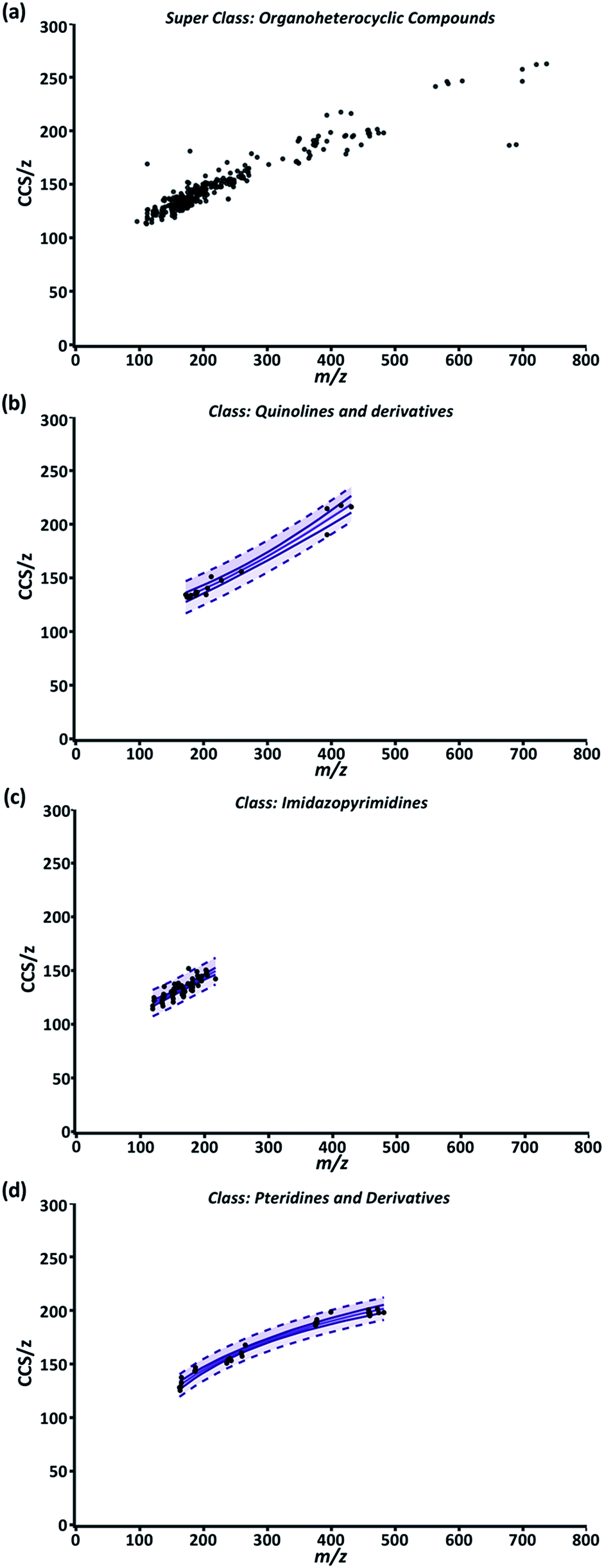 | ||
| Fig. 3 (a) Compendium GUI output of all ion entries within the “Organoheterocyclics” super class. (b) “Quinolines and derivatives” class; and a 4P regression. (c) “Imidazopyrimidines” class; and a 4P regression. (d) “Pteridines and derivatives” class; and a PF regression. For (b–d), the center solid line is the regression model, outer solid lines are 99% CI and the dash lines are 99% PI. | ||
Fig. 3 is a representative example of this data correlation process. It depicts the super class “Organoheterocyclic compounds” which contain many human metabolites and natural products. Three classes within “Organoheterocyclic compounds” are shown in Fig. 3b–d. The “Quinolines and derivatives” (Fig. 3b) and “Imidazopyrimidines” classes (Fig. 3c) were best fit by a 4P regression model. The “Pteridines and derivatives” class (Fig. 3d) was fit best by the PF regression. In these cases, data fit regressions and corresponding CIs and PIs define the CCS/z vs. m/z space that 99% of data for diazines, imidazopyrimidines, and pteridines and derivatives should occupy. While current AICc values indicate these models are appropriate, the specificity and predictability of these intervals will improve with the inclusion of more data and further delineation of each class into subclasses.
In the compendium, the 99% confidence and predictive intervals included in the data projections are calculated directly from the compendium data, therefore the majority of the empirical measurements within the dataset will fall within these intervals. As these bands represent a probability, there remains the possibility that CCS values for compound standards will fall outside of these projections, and users should examine these cases on an individual basis to determine if CCS values are repeatably and reproducibly outside of the predicted range. For example, multimers dissociating occurring after the ion mobility measurement but prior to mass analysis (i.e., post-mobility ion activation) would lead to a larger than expected drift time and corresponding CCS. Additionally, CCS values for unknown analytes/isomers obtained from untargeted experiments represent previously unmeasured peak features which could fall outside of the interval bands. In these scenarios, the user should exercise caution in determining if the predicted structural class is appropriate.
The compendium as an identification filter
To test the predictability and filtering abilities of the compendium, metabolites were extracted from control human serum analyzed using LC-MS or LC-IM-MS workflows. In the LC-MS data, 4719 deconvoluted compounds were observed. In total, 955 tentative identifications were matched using conservative criteria for exact mass (<10 ppm) and isotope distribution (70%) using Metlin metabolomics and LipidBlast databases.55,56 In order to append drift time values to these tentative identifications, an in-house Python script (available online) was developed.45 Using this script, we can extract drift times at a rate of 4 × 10⁵ measurements in ∼1 h per sample. Drift times from each of the three technical replicates were aligned to the tentative identifications based on retention time and m/z. In these data, a majority of the aligned drift times were self-consistent with an RSD ≤ 1%. The drift times were averaged and used to calculate CCS/z values using the single-field extension of the Mason–Schamp relationship. The annotated serum data is represented in Fig. 4a (labeled “tentatively identified serum metabolites”). Superimposing the serum data over the Unified CCS compendium data (Fig. 4a) illustrates that the tentatively identified compounds have equivalent mobility–mass correlations as known chemical compounds.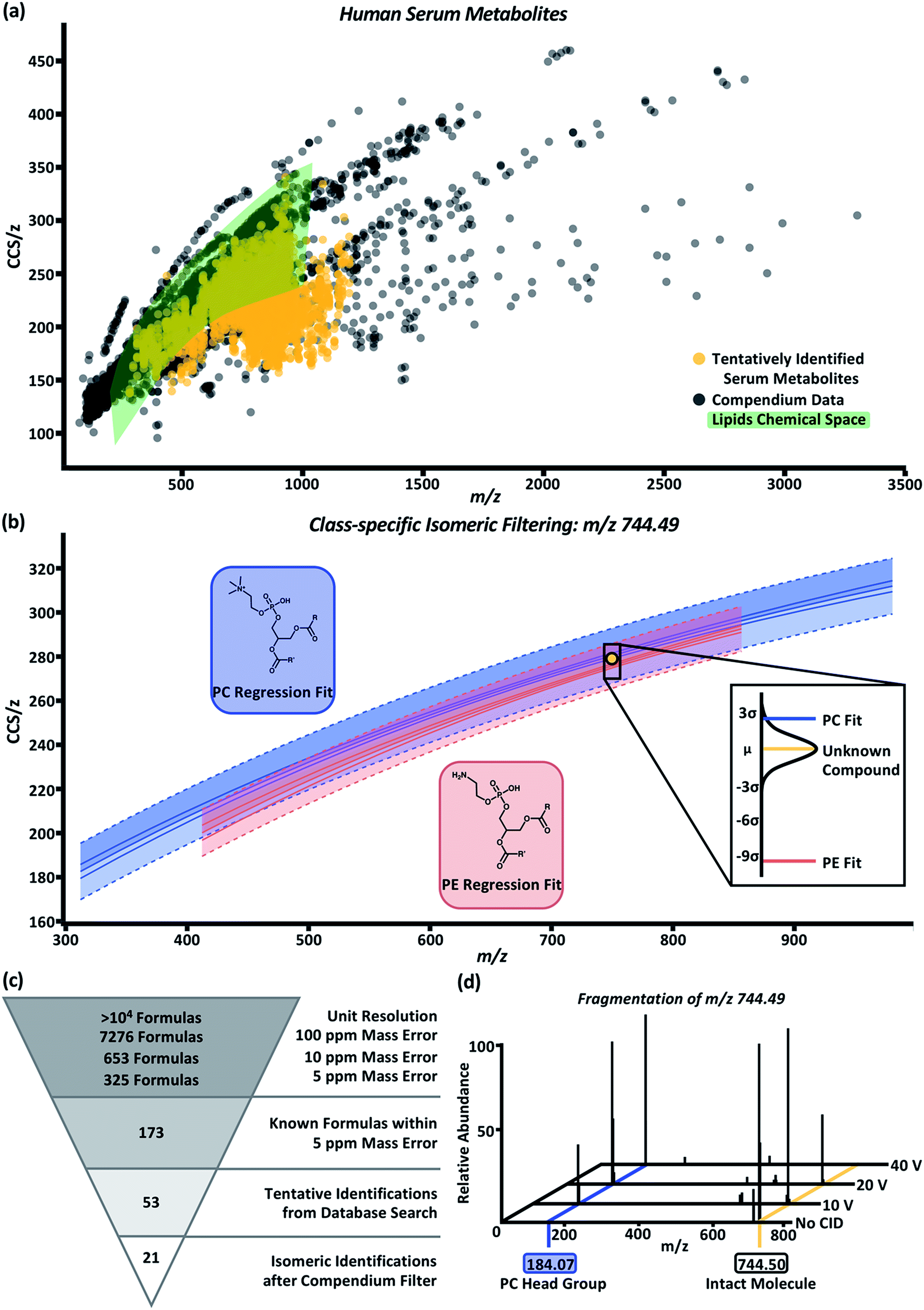 | ||
| Fig. 4 (a) Overlay of human serum metabolites (gold) with the compendium (black). Green area represents CCS/z vs. m/z space occupied by any and all lipid subsets within the compendium. (b) Example plot for class-specific filtering of an unknown serum compound, m/z 744.49 and CCS 278.2 Å2 (gold circle), tentatively identified as a PC (blue regression model) or PE (red regression model). The probability of the unknown compound's class falling within the PC or PE class is shown in the call out box. Based on distance from the mean calculations, the compound falls within 2.54 standard deviations of the PC regression model and 9.44 standard deviations of the PE regression model which indicates the unknown compounds has a higher probability of being a PC than a PE. (c) Molecular identification workflow for the unknown compound depicted in panel (b). After compendium filtering, identifications were reduced to 21 PC isomers with the m/z 744.49. (d) Fragmentation of the isolated m/z 744.49 at CID 0 V, 10 V, 20 V, and 40 V. An increase in the intensity for m/z 184.07, corresponding to the phosphocholine head group mass, is observed with increase in collision voltage. | ||
For proof-of-concept purposes, the serum data was subset into compounds tentatively identified as lipids. Compounds in the green highlighted area of Fig. 4a represent the CCS/z vs. m/z space within the Unified CCS compendium containing any and all lipid regressions generated for data in the “Lipids and lipid-like molecules” super class. In total, 550 compounds present in the serum sample were tentatively identified as lipids; and 422 of these compounds overlapped with at least one of the lipid class and/or lipid subclass regression models. Distance from the mean values were then calculated to prioritize the probability that a serum compound belonged to a given lipid class. An example of this process is depicted in Fig. 4b for the compound with m/z 744.49 and CCS 278.2 Å2 (gold circle). Potential tentative identifications for m/z 744.49 included 53 isomers of glycerophosphocholines (PC) and glycerophosphoethanolamines (PE). This unknown compound (gold line, Fig. 4b call-out box) was 2.54 standard deviations away from the PC subclass regression model (blue line, Fig. 4b call-out box) and 9.44 standard deviations from the PE subclass regression model (red line, Fig. 4b call-out box). At 2.54 standard deviations, this compound was within the 99% confidence interval of the PC subclass regression model and had a difference of about 1.5 Å2 from the mean CCS/z value of PCs at m/z 744. Using this Unified CCS compendium, there is more data to suggest the unknown compound's tentative identity is a PC. Thus, a putative identification and higher confidence in its assignment can be attributed.
The molecular identification workflow for m/z 744.49 is summarized in Fig. 4c. The m/z 744.49 was deconvoluted to its neutral mass of 705.53 Da. At unit resolution, there are tens of thousands of potential chemical formulas with a mass of 705 Da. Within 100 ppm mass error of 705.53 Da, there are 7276 possible chemical formulas. Subsequently, there are 653 chemical formulas within 10 ppm mass error and 325 chemical formulas within 5 ppm mass error (the observed mass error). Of these 325 formulas, 173 are known compounds found in the PubChem database. Heuristic filtering based on instrumentation mass accuracy, mass defect, isotope distribution, and information from orthogonal separations enables tentative identification of compounds with a specified level of confidence. In this example, 53 tentative PC and PE identifications were returned after heuristic filtering through Progenesis QI. Using the compendium, this list can be further narrowed into 21 PC isomers with the neutral mass 705.53 and m/z 744.49.
To validate our PC prediction, m/z 744.49 underwent mass isolation from the serum matrix and was fragmented using collision induced dissociation at 0 V, 10 V, 20 V, and 40 V. The mass spectra, shown in Fig. 4d, demonstrate the increase in the intensity of m/z 184.07, the signature m/z of a phosphocholine head group, as collision energy increased. While further investigation using chemical standards can lead to high-confidence identifications of unknown compounds, using the CCS filtering workflow presented here allows investigators to achieve high confidence in assigning the chemical class to an unknown molecule using IM-MS datasets. This predictive ability is expected to be particularly important for chemical class and structure annotation of isomers belonging to known compounds from which CCS information has not been previously measured (i.e., an “unknown unknown” isomer), as is the case for the majority of human metabolites which are expected to be isomeric but current undiscovered.59
Conclusions
In this work, we illustrate the utility of IM-MS in quantitatively characterizing biochemical species using a Unified CCS compendium. Prior to this work, quantitative CCS libraries have been limited in scope to a narrow range of chemical classes, polarities, and adduct types. Therefore, we curated a Unified CCS compendium obtained from chemical standards representing a wide variety of structures spanning 14 super classes, 80 classes, and 157 subclasses. We anticipate subsequent contributions from the IM-MS community; and therefore, the informatics infrastructure developed was designed to accommodate future expansion. The current biochemical species contained within the Unified CCS compendium enabled generation of optimized nonlinear regression models with CI and PI for 48 classes and subclasses. These models enabled filtering and prediction of unknown biochemical species. The capabilities demonstrated in this manuscript establish a foundation for utilizing CCS/z as an additional molecular characterization dimension. The Unified CCS compendium was used to predict and identify unknown chemical species that originated from a serum sample. Future work will focus on expanding the number of entries in the compendium to improve predictive power.We aim for the Unified CCS compendium to be a collaborative effort of the IM-MS community and invite contributions to this open-access repository for quality-controlled CCS measurements. Specific guidelines for submitting data are found in the ESI (Section S2†). While the compendium is initially designed to only include DTIMS data, considerations for adding CCS information obtained from other IM techniques will be included in future iterations. The standardized DTIMS CCS measurements contained within the compendium can serve as calibrant reference values for other IM techniques, which will ultimately enable the incorporation of more CCS data into this body of work.
Conflicts of interest
The authors declare no competing financial interest.Acknowledgements
The authors would like to acknowledge Erin S. Baker and colleagues at the Pacific Northwest National Laboratory, as well as James N. Dodds, Caleb B. Morris, and Charles M. Nichols at Vanderbilt University for their efforts in acquiring data within the compendium; and Timo Sachsenberg at the University of Tübingen for his guidance in methods for large scale drift time extraction analyses. Additionally, the authors would like to acknowledge John C. Fjeldsted of Agilent Technologies for his collaborative efforts and expertise. Financial support for this research was provided by the National Institutes of Health (NIH NIGMS R01GM092218 and NIH NCI 1R03CA222452-01) and the NIH supported Vanderbilt Chemical Biology Interface training program (5T32GM065086-16). This work was supported in part using the resources of the Center for Innovative Technology (CIT) at Vanderbilt University.Notes and references
- D. Houle, D. R. Govindaraju and S. Omholt, Nat. Rev. Genet., 2010, 11, 855–866 CrossRef CAS PubMed.
- J. C. May, R. L. Gant-Branum and J. A. McLean, Curr. Opin. Biotechnol., 2016, 39, 192–197 CrossRef CAS PubMed.
- J. C. May and J. A. McLean, Annu. Rev. Anal. Chem., 2016, 9, 387–409 CrossRef PubMed.
- S. M. Paul, D. S. Mytelka, C. T. Dunwiddie, C. C. Persinger, B. H. Munos, S. R. Lindborg and A. L. Schacht, Nat. Rev. Drug Discovery, 2010, 9, 203–214 CrossRef CAS PubMed.
- R. A. Quinn, J. A. Navas-molina, E. R. Hyde, J. Song, Y. Vázquez-baeza, G. Humphrey, J. Gaffney, J. J. Minich, A. V. Melnik, J. Herschend, J. Dereus, A. Durant, R. J. Dutton, M. Khosroheidari and C. Green, mSystems, 2016, 1, e00038-1–6 CrossRef PubMed.
- R. Chen, G. I. Mias, J. Li-Pook-Than, L. Jiang, H. Y. K. Lam, R. Chen, E. Miriami, K. J. Karczewski, M. Hariharan, F. E. Dewey, Y. Cheng, M. J. Clark, H. Im, L. Habegger, S. Balasubramanian, M. O'Huallachain, J. T. Dudley, S. Hillenmeyer, R. Haraksingh, D. Sharon, G. Euskirchen, P. Lacroute, K. Bettinger, A. P. Boyle, M. Kasowski, F. Grubert, S. Seki, M. Garcia, M. Whirl-Carrillo, M. Gallardo, M. A. Blasco, P. L. Greenberg, P. Snyder, T. E. Klein, R. B. Altman, A. J. Butte, E. A. Ashley, M. Gerstein, K. C. Nadeau, H. Tang and M. Snyder, Cell, 2012, 148, 1293–1307 CrossRef CAS PubMed.
- J. S. D. Zimmer, M. E. Monroe, W. J. Qian and R. D. Smith, Mass Spectrom. Rev., 2006, 25, 450–482 CrossRef CAS PubMed.
- X. Zheng, R. Wojcik, X. Zhang, Y. M. Ibrahim, K. E. Burnum-Johnson, D. J. Orton, M. E. Monroe, R. J. Moore, R. D. Smith and E. S. Baker, Annu. Rev. Anal. Chem., 2017, 10, 71–92 CrossRef CAS PubMed.
- J. A. McLean, B. T. Ruotolo, K. J. Gillig and D. H. Russell, Int. J. Mass Spectrom., 2005, 240, 301–315 CrossRef CAS.
- K. M. Hines, J. C. May, J. A. McLean and L. Xu, Anal. Chem., 2016, 88, 7329–7336 CrossRef CAS PubMed.
- W. B. Ridenour, M. Kliman, J. A. McLean and R. M. Caprioli, Anal. Chem., 2010, 82, 1881–1889 CrossRef CAS PubMed.
- S. M. Stow, T. J. Causon, X. Zheng, R. T. Kurulugama, T. Mairinger, J. C. May, E. E. Rennie, E. S. Baker, R. D. Smith, J. A. McLean, S. Hann and J. C. Fjeldsted, Anal. Chem., 2017, 89, 9048–9055 CrossRef CAS PubMed.
- C. B. Lietz, Q. Yu and L. Li, J. Am. Soc. Mass Spectrom., 2014, 25, 2009–2019 CrossRef CAS PubMed.
- W. B. Struwe, K. Pagel, J. L. P. Benesch, D. J. Harvey and M. P. Campbell, Glycoconj. J., 2016, 33, 399–404 CrossRef CAS PubMed.
- K. M. Hines, D. H. Ross, K. L. Davidson, M. F. Bush and L. Xu, Anal. Chem., 2017, 89, 9023–9030 CrossRef CAS PubMed.
- Z. Zhou, J. Tu, X. Xiong, X. Shen and Z. J. Zhu, Anal. Chem., 2017, 89, 9559–9566 CrossRef CAS PubMed.
- M. Hernández-Mesa, B. Le Bizec, F. Monteau, A. M. García-Campaña and G. Dervilly-Pinel, Anal. Chem., 2018, 90, 4616–4625 CrossRef PubMed.
- X. Zheng, N. Aly, Y. Zhou, K. Dupuis, A. Bilbao, V. Paurus, D. J. Orton, R. Wilson, S. Payne, R. D. Smith and E. S. Baker, Chem. Sci., 2017, 8, 7724–7736 RSC.
- Z. Zhou, X. Shen, J. Tu and Z.-J. Zhu, Anal. Chem., 2016, 88, 11084–11091 CrossRef CAS PubMed.
- G. Paglia, J. P. Williams, L. Menikarachchi, J. W. Thompson, R. Tyldesley-Worster, S. Halldórsson, O. Rolfsson, A. Moseley, D. Grant, J. Langridge, B. O. Palsson and G. Astarita, Anal. Chem., 2014, 86, 3985–3993 CrossRef CAS PubMed.
- L. Righetti, A. Bergmann, G. Galaverna, O. Rolfsson, G. Paglia and C. Dall'Asta, Anal. Chim. Acta, 2018, 1014, 50–57 CrossRef CAS PubMed.
- C. R. Goodwin, L. S. Fenn, D. K. Derewacz, B. O. Bachmann and J. A. McLean, J. Nat. Prod., 2012, 75, 48–53 CrossRef CAS PubMed.
- R. Lian, F. Zhang, Y. Zhang, Z. Wu, H. Ye, C. Ni, X. Lv and Y. Guo, Anal. Methods, 2018, 10, 749–756 RSC.
- M. Chai, M. N. Young, F. C. Liu and C. Bleiholder, Anal. Chem., 2018, 90, 9040–9047 CrossRef CAS PubMed.
- V. Gabelica and E. Marklund, Curr. Opin. Chem. Biol., 2018, 42, 51–59 CrossRef CAS PubMed.
- I. Blaženović, T. Kind, J. Ji and O. Fiehn, Metabolites, 2018, 8, 31 CrossRef PubMed.
- J. Ma, C. P. Casey, X. Zheng, Y. M. Ibrahim, C. S. Wilkins, R. S. Renslow, D. G. Thomas, S. H. Payne, M. E. Monroe, R. D. Smith, J. G. Teeguarden, E. S. Baker and T. O. Metz, Bioinformatics, 2017, 33, 2715–2722 CrossRef CAS PubMed.
- B. X. Maclean, B. S. Pratt, J. D. Egertson, M. J. Maccoss, R. D. Smith and E. S. Baker, J. Am. Soc. Mass Spectrom., 2018 DOI:10.1007/s13361-018-2028-5.
- B. Pratt, M. Horowitz-gelb, J. W. Thompson, E. Baker, J. W. Thompson, M. J. Maccoss and B. Maclean, in 65th Annual Conference for the American Society of Mass Spectrometry, American Society for Mass Spectrometry, Indianapolis, IN, 2017 Search PubMed.
- B. D. Ripley, Pattern Recognition and Neural Networks, Cambridge University Press, Cambridge, UK, 1996 Search PubMed.
- S. M. Colby, D. G. Thomas, J. R. Nunez, D. J. Baxter, K. R. Glaesemann, M. Brown, M. A. Pirrung, N. Govind, J. G. Teeguarden, T. O. Metz and S. Ryan, arXiv:1809.08378 [q-bio.BM].
- Mclean Research Group, CCS compendium, http://https://lab.vanderbilt.edu/mclean-group/collision-cross-section-database/.
- C. M. Nichols, J. C. May, S. D. Sherrod and J. A. McLean, Analyst, 2018, 143, 1556–1559 RSC.
- J. C. May, C. R. Goodwin, N. M. Lareau, K. L. Leaptrot, C. B. Morris, R. T. Kurulugama, A. Mordehai, C. Klein, W. Barry, E. Darland, G. Overney, K. Imatani, G. C. Stafford, J. C. Fjeldsted and J. A. McLean, Anal. Chem., 2014, 86, 2107–2116 CrossRef CAS PubMed.
- J. N. Dodds, J. C. May and J. A. Mclean, Anal. Chem., 2017, 89, 952–959 CrossRef CAS PubMed.
- J. C. May, E. Jurneczko, S. M. Stow, I. Kratochvil, S. Kalkhof and J. A. McLean, Int. J. Mass Spectrom., 2017, 427, 79–90 CrossRef PubMed.
- K. L. Leaptrot, J. C. May, J. N. Dodds. J. A. McLean and Nat. Commun., submitted Search PubMed.
- C. M. Nichols, J. N. Dodds, B. S. Rose, J. A. Picache, C. B. Morris, S. G. Codreanu, J. C. May, S. D. Sherrod and J. A. McLean, Anal. Chem., 2018 DOI:10.1021/acs.analchem.8b04322.
- E. A. Mason and E. W. McDaniel, Transport Properties of Ions in Gases, John Wiley & Sons, Ltd., New York City, NY, 1988 Search PubMed.
- W. F. Siems, L. A. Viehland and H. H. Hill, Anal. Chem., 2012, 84, 9782–9791 CrossRef CAS PubMed.
- R. Core Team, A language and environment for statistical computing. R Foundation for Statistical Computing, https://www.r-project.org/ Search PubMed.
- V. Gabelica, C. Alfonso, P. E. Barran, J. L. P. Benesch, C. Bleiholder and M. T. Bowers, et al. , ChemRxiv, 2018 DOI:10.26434/chemrxiv.7072070.v2.
- Y. Djoumbou Feunang, R. Eisner, C. Knox, L. Chepelev, J. Hastings, G. Owen, E. Fahy, C. Steinbeck, S. Subramanian, E. Bolton, R. Greiner and D. S. Wishart, J. Cheminf., 2016, 8, 1–20 Search PubMed.
- H. J. Feldman, M. Dumontier, S. Ling, N. Haider and C. W. V. Hogue, FEBS Lett., 2005, 579, 4685–4691 CrossRef CAS PubMed.
- McLean Research Group Github, https://github.com/McLeanResearchGroup.
- C. B. Morris, J. C. May and J. A. McLean, in 62th Annual Conference for the American Society of Mass Spectrometry, Baltimore, MD, 2014 Search PubMed.
- J. C. May, C. B. Morris and J. A. McLean, Anal. Chem., 2017, 89, 1032–1044 CrossRef CAS PubMed.
- K. P. Burnham and D. R. Anderson, Model Selection and Multimodel Inference: A Practical Information-Theoretic Approach, Springer-Verlag, New York City, NY, 2nd edn, 2002, vol. 172 Search PubMed.
- A. N. Spiess and N. Neumeyer, BMC Pharmacol., 2010, 10, 1–11 Search PubMed.
- C. Sievert, C. Parmer, T. Hocking, S. Chamberlain, K. Ram, M. Corvellec and P. Despouy, Create Interactive Web Graphics via ‘plotly.js’, https://cran.r-project.org/package=plotly Search PubMed.
- H. Wickham, ggplot2: Elegant Graphics for Data Analysis, http://ggplot2.org Search PubMed.
- M. Dowle and A. Srinivasan, data.table: Extension of ‘data.frame’, https://cran.r-project.org/package=data.table.
- H. Wickham, J. Stat. Software, 2011, 40, 1–29 Search PubMed.
- W. Chang, J. Cheng, J. Allaire, Y. Xie and J. McPherson, shiny: Web Application Framework for R, https://cran.r-project.org/package=shiny Search PubMed.
- C. A. Smith, G. O'Maille, E. J. Want, C. Qin, S. A. Trauger, T. R. Brandon, D. E. Custodio, R. Abagyan and G. Siuzdak, Ther. Drug Monit., 2005, 27, 747–751 CrossRef CAS PubMed.
- T. Kind, K. H. Liu, D. Y. Lee, B. Defelice, J. K. Meissen and O. Fiehn, Nat. Methods, 2013, 10, 755–758 CrossRef CAS PubMed.
- M. C. Chambers, B. MacLean, R. Burke, D. Amodei, D. L. Ruderman, S. Neumann, L. Gatto, B. Fischer, B. Pratt, J. Egertson, K. Hoff, D. Kessner, N. Tasman, N. Shulman, B. Frewen, T. A. Baker, M. Y. Brusniak, C. Paulse, D. Creasy, L. Flashner, K. Kani, C. Moulding, S. L. Seymour, L. M. Nuwaysir, B. Lefebvre, F. Kuhlmann, J. Roark, P. Rainer, S. Detlev, T. Hemenway, A. Huhmer, J. Langridge, B. Connolly, T. Chadick, K. Holly, J. Eckels, E. W. Deutsch, R. L. Moritz, J. E. Katz, D. B. Agus, M. MacCoss, D. L. Tabb and P. Mallick, Nat. Biotechnol., 2012, 30, 918–920 CrossRef CAS PubMed.
- J. J. Faraway, Practical Regression and Anova using R, 3rd edn, 2002 Search PubMed.
- D. S. Wishart, Y. D. Feunang, A. Marcu, A. C. Guo, K. Liang, R. Vázquez-Fresno, T. Sajed, D. Johnson, C. Li, N. Karu, Z. Sayeeda, E. Lo, N. Assempour, M. Berjanskii, S. Singhal, D. Arndt, Y. Liang, H. Badran, J. Grant, A. Serra-Cayuela, Y. Liu, R. Mandal, V. Neveu, A. Pon, C. Knox, M. Wilson, C. Manach and A. Scalbert, Nucleic Acids Res., 2018, 46, D608–D617 CrossRef CAS PubMed.
Footnote |
| † Electronic supplementary information (ESI) available. See DOI: 10.1039/c8sc04396e |
| This journal is © The Royal Society of Chemistry 2019 |