Algorithms for the self-optimisation of chemical reactions

Abstract

Self-optimising chemical systems have experienced a growing momentum in recent years, with the evolution of self-optimising platforms leading to their application for reaction screening and chemical synthesis. With the desire for improved process sustainability, self-optimisation provides a cheaper, faster and greener approach to the chemical development process. The use of such platforms aims to enhance the capabilities of the researcher by removing the need for labor-intensive experimentation, allowing them to focus on more challenging tasks. The establishment of these systems have enabled opportunities for self-optimising platforms to become a key element of a laboratory's repertoire. To enable the wider adoption of self-optimising chemical platforms, this review summarises the history of algorithmic usage in chemical reaction self-optimisation, detailing the functionality of the algorithms and their applications in a way that is accessible for chemists and highlights opportunities for the further exploitation of algorithms in chemical synthesis moving forward.

---

Introduction

The numerous advantages of continuous flow chemistry over conventional batch chemistry are becoming apparent to a growing number of synthetic chemists.^1,2 Properties such as enhanced heat and mass transfer,^3,4 safer use of hazardous reagents⁵ and an extended operating window⁶ enable reactions that are difficult or even impossible in batch to be achieved relatively easily.⁷ In addition, automation is readily implemented into flow systems via in-line monitoring, offering a greater degree of reliability and reaction control.^8,9

These advances in the automation of laboratory equipment have simultaneously led to a rise in the use of algorithms in chemistry.^10,11 With developments in automation enabling chemists to make better use of the human resource by assigning routine, labour intensive tasks to machines.^12,13 More recently, machine learning algorithms have been applied to more challenging tasks, such as the discovery of new chemical reactivity¹⁴ and the prediction of reaction outcomes.¹⁵

Automated flow systems are able to search large regions of experimental space in relatively short periods of time, making them well suited for optimisation problems.^16,17 Optimising processes by combining flow reactors, process analytics and optimisation algorithms is known as ‘self-optimisation’. The reaction mixture is analysed and the responses are supplied to an optimisation algorithm. The algorithm then generates the next set of conditions to explore based on the results of the previous experiments, thereby creating a feedback loop.¹⁸ Intelligent analysis of the experimental space reduces the number of experiments required, providing a faster, cheaper and ‘greener’ method for process development. Self-optimising systems provide an enabling technology for efficient optimisation of expensive-to-evaluate chemical systems. As such, algorithms used in self-optimisation typically focus on minimising the number of experiments and material consumed during the optimisation process. Given that the algorithm selected by the user has a significant influence on the efficiency of the optimisation, there will remain a continued interest in the development of algorithms for self-optimising systems.

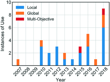
Self-optimising systems are developed at the interface between chemistry, chemical engineering and computer science. For self-optimising systems to become more commonplace in research laboratories, the end-user (e.g. chemists) require a basic knowledge of the types of algorithms available. However, reviews in this area have to date focused primarily on the monitoring of reactions, and less on the algorithms employed.^19,20 In this review, we provide an overview of the algorithms which have been used for self-optimisation to date (Fig. 1), including explanations designed to aid chemists in their choice of the most appropriate algorithm for a given synthetic challenge.

Fig. 1 A summary of algorithms used in self-optimising chemical platforms.

Local optimisation

Model-based

Design of experiments (DoE) has been studied and used for chemical process optimisation and screening for many decades.²¹ This approach is used to determine a set of experiments which will efficiently identify the important factors affecting the chemical system, as well as ascertaining how the differing factors interact with each other. This statistical framework allows optimum regions of experimental space to be located for further exploration through the construction of a response surface; where a response surface describes the relationship between experimental variables (e.g. reaction temperature, time, pH etc.) and a response (e.g. yield). The literature behind the designs is well understood and known throughout the chemical industry and academia where it is used readily.^22,23

Methods to improve the standard rigid DoE design, to allow for adjustment based on the responses from a given process, have been attempted in a self-optimising chemical environment. The Jensen group first utilised an optimal DoE approach for the optimisation of the alkylation of 1,2-diaminocyclohexane for discrete (e.g. solvents, catalysts, ligands) and continuous variables (e.g. reaction time, temperature, reagent equivalents).²⁴ The optimisation was initialised using a screening set of experiments, from which a linear response surface was fitted. In performing only screening experiments, elucidation of potential response curvature is not possible, however, this is contrasted by the conservation of resources. Following initialisation, further experiments were performed focusing on determining the optimum point for each solvent. Fitting of a quadratic model was performed and a paired 2-sample t-test allowed for the elimination of poorly performing solvents. Optimal regions for the remaining solvents were determined by applying G-optimality, which aims to design experiments which minimise the maximum variance of the models predicted values.²⁵

The algorithm has been further refined, initially enhancing the handling of discrete variables via the addition of a mixed integer nonlinear programming (MINLP) approach,²⁶ with discrete variables removed when performance was poor. MINLP refers to optimisation tasks involving both continuous and discrete variables, with nonlinearities in the response. Further alterations were made to improve the initial space filling experimental design, being led by D-optimality, with additional improvements to the discrete variable reduction process.^27,28 D-optimal designs seek to minimise the covariance (uncertainty) of the parameter estimates for a specific model.²⁹ For the catalytic reaction studied, the authors assumed the system could be modelled as a logarithmic model derived from the assumption that the reaction had a single rate determining step. The requirement for an assumed model derivation could present an issue for the application of the algorithm in kinetically complex systems and for general purpose use without a priori knowledge.¹⁸ Additionally, the use of a paired 2-sample t-test for solvent elimination has the potential to miss the best conditions due to synergistic effects. To date this algorithm presents the only documented self-optimisation of both discrete and continuous variables in a chemical system, with scope for the field to expand in this area.

Black-box

Black-box optimisation techniques are defined as methods requiring no mechanistic understanding of the process to perform the optimisation task. The Nelder–Mead simplex (NMSIM) algorithm is an example of a black-box local optimisation method used to determine the maximum (or minimum) of a single-objective function (a response being optimised). This is achieved by means of using convex polyhedra formed of n + 1 vertices (where n is the number of variables).³⁰ The polyhedron, or simplex, explores the feasible design space set by the user. The algorithm begins by conducting either user-defined or random experiments within a given area of the design space, with each vertex of a polyhedron representing an experiment with an evaluation of the response function. The worst performing vertex is then replaced at each iteration of the algorithm with another vertex via a geometric transformation, resulting in a new simplex that explores a new point in the design space. This approach locates areas with a better response and hence successive simplex iterations converge on a local optima. The method of defining the new vertex is based on five geometrical transformations of a current simplex, outlined in Fig. 2, which depict two-dimensional transformations that can be extrapolated to higher dimensions.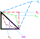

Fig. 2 The different geometric transformations of the Nelder–Mead simplex: inside contraction (X_IC), multiple contraction (MC), outside contraction (X_OC), reflection (X_R) and expansion (X_E).

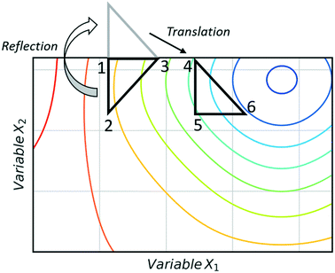
Fig. 3 shows an example of how NMSIM can find the local minimum of a response function in a two-variable design space. The initial vertices of simplex 1 are evaluated via the response function, then the worst vertex is replaced via reflection to form simplex 2. Similarly, the worst vertex of simplex 2 is replaced via reflection to form simplex 3. These successive transformations enable the simplex algorithm to converge on an optimum. The optimisation typically stops when a better response function evaluation cannot be found, indicating that a local optimum has been identified. One of the first times this algorithm was applied to self-optimisation was in the Heck reaction, and represented one of the earliest examples of a self-optimising chemical platform.³¹ A publication by Krishnadasan et al. from the same year shows the use of simplex methods for optimisation of nanoparticle production. The authors utilise a dynamic simplex to apply compensation in the case of system-drift (unforeseen changes in the system).³² Further work by Cronin and co-workers successfully coupled the algorithm with in-line NMR to optimise an imine synthesis, with a total of 29 experiments, utilising a custom cost function.³³

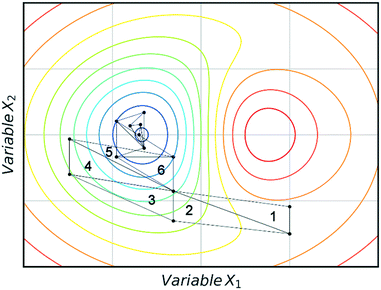Fig. 3 An example of a two-variable design space with arbitrary variables and a mapped response surface, showing how NMSIM converges on the minimum. Minima (blue), maxima (red).

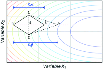
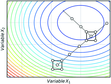
The super modified simplex algorithm (SMSIM) is an adaptation of NMSIM, originally introduced by Routh et al.,³⁴ whereby polynomial fitting of data points determines the optimum simplex transformations. As these transformations are based on predictions from the polynomials generated, the algorithm can accelerate across areas of low interest. Fig. 4 shows an initial simplex formed of data points 1, 2 and 3, where 3 is the worst result. The midpoint of 1 and 2 is then measured as 4, which is the ‘centroid’. The centroid is the point at which vertex 3 will be reflected through at distance X_Rα to vertex 5, which is also measured. A second order polynomial through data points 3, 4 and 5 is then constructed and extrapolated to identify the optimum expansion distance X_Rβ to vertex 6.³⁵ Many notable modifications to NMSIM have been reported by Felpin et al. which were used in the self-optimisation of the Heck–Matsuda reaction and in the natural product synthesis of carpanone, over four stages with a total of 66 experiments.^36,37 These modifications include: boundary and linear constraints on variables (such as temperature, or temperature given a concentration), dimensionality reduction upon exploring boundaries, dimension recovery to re-enter the design space (Fig. 5), diversification by searching unexplored regions and the ability to have multiple termination criteria (such as when all material has been consumed). Other modifications to NMSIM such as complex method³⁸ have also been used for self-optimisation, such as in the amidation of 3-cyanopyridine.³⁹ This algorithm works in a very similar way to SMSIM, however, instead of basing the expansion distances on predicted optimal regions via polynomial fitting, an iterative process is employed. This iterative process begins by measuring a vertex at a given expansion distance. If the measurement is worse than the current data points, it is rejected. Additional measurements are then taken at incrementally shorter distances along the same direction, until a better evaluation is found. Gradient-based methods are another form of local optimisation that typically converge on the optimum by following the initial trajectory of the local response surface. The steepest descent method⁴⁰ is a gradient-based algorithm first used in a chemical system by McMullen and Jensen in combination with DoE for the optimisation of a Knoevenagel condensation reaction.⁴¹ In this method, an initial 2^k orthogonal design (where k is the number of variables) or central composite design (CCD) DoE is performed around a particular starting point. A local response surface is then modelled, from which the gradients are calculated. Further experiments are performed along the trajectory of the gradient until the response function value worsens, indicating that the optimum has been passed or that a change of search direction is necessary to proceed, as shown in Fig. 6. Modifications to the steepest descent method, such as conjugate gradient and Armijo conjugate gradient, have also been used in the self-optimisation of the Paal–Knorr synthesis.⁴²

Fig. 4 An example showing how a polynomial fit to the data (red dashed line) predicts the optimum expansion point to the next simplex vertex, resulting in the new simplex expansion (dashed line) towards the minimum (blue contour).

Fig. 5 A translation of the reflected simplex of 1-2-3 into an infeasible region occurs in order to rebuild a simplex of the same geometry (4-5-6) within the imposed boundary constraints, hence recovering the dimensions of the search. Minima (blue), maxima (red).

Fig. 6 A steepest descent method minimisation, where an initial point and 2^k orthogonal design are performed, followed by further experiments along the trajectory of highest gradient towards the optimum. Minima (blue), maxima (red).

The conjugate gradient algorithm utilises the weighted sum of the last search direction and the direction calculated via the steepest descent method to determine the next iteration. This prevents large direction adjustments which are less likely to lead the algorithm through difficult response surface terrain.⁴³ The Armijo algorithm differs by implementing an Armijo-type line search.⁴⁴ This varies the step size along each trajectory, which was shown to out-perform the other steepest descent algorithms by reaching a similar optimum in fewer experiments.^41,42 Where gradient information is available this can offer faster convergence, however, this can be complicated in the presence of experimental noise and the need to fit a mathematical surface. Real-time analysis of transient experiments in the future may enable experimentally measured gradients to be utilised although to the authors' knowledge this has not been demonstrated yet.

Many local optimisation algorithms are typically fast to converge on an optimum, as each successive iteration of the algorithm makes progressive improvements by moving perpendicularly to the contour of the response-surface. Variants of both the simplex and steepest descent algorithms have been shown to converge on optima within a self-optimising reaction system, each with their own advantages in terms of robustness and experimental efficiency. The disadvantage of using local optimisation tools is when there is no a priori knowledge about the reaction system; as the complexity of the system arising from variable–variable interactions can lead to multiple optima. In these cases, there is no guarantee that the global optimum will be found over a local optima before termination.

When considering a local optimisation algorithm it must therefore be assumed that the chemical system of interest has a single optimum, otherwise a global optimisation tool may be more relevant.

Consideration of optimisation time may also be worthwhile when selecting a local or global optimiser. Due to global searching, experimental points are on average further apart in the experimental space, meaning the reactor system can take correspondingly longer to reach the new conditions.⁴⁵

Global optimisation

An algorithm's ability to locate the optimum despite the inherent experimental noise of chemical systems is crucial for self-optimising platforms. As there are no noise-handling capabilities inbuilt in local search algorithms, the presence of significant noise can be detrimental to the speed of identifying the optimum. Considerable noise in a system can lead to local optimisation techniques, such as simplex, prematurely terminating at a point away from the true optimum of the system. As many global optimisers attempt to facilitate noise, their convergence on the optimum may be more efficient in notably noisy systems.

Stable Noisy Optimisation by Branch and Fit (SNOBFIT) is a global optimisation algorithm for bound constrained noisy optimisation of objective functions.⁴⁶ To date, this is the only single-objective optimiser which has been successfully implemented in self-optimisation. It is a derivative-free optimisation method, which means that it requires no gradient information of the objective function being optimised. The algorithm uses a combination of stochastic linear and quadratic surrogate models to determine the optimum point of the system. A surrogate model is an approximate model that maps the process inputs to an objective function.⁴⁷ They provide a cheap alternative which can be called in lieu of the parent function to improve optimisation efficiency, with the stochastic nature of the models enabling the algorithm to handle noise effectively.

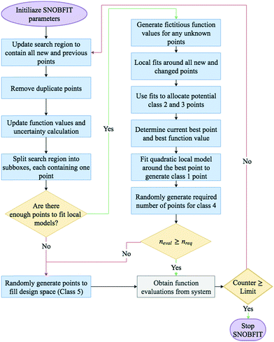
A basic flow diagram detailing a simplified overview of SNOBFIT is shown in Fig. 7. The algorithm generates points in five different classifications:

Fig. 7 Flow diagram for a call of the SNOBFIT algorithm. n_eval is the current number of points for the following iteration SNOBFIT has generated. n_req is the required number of points to be generated for each call of the algorithm, this is set by the user.

- Class 1: the point that minimises the local quadratic model around the current best point (x_best). It contains at most one point

- Class 2: are points that are approximate local minimisers. If there are no local points then no points in class 2 are generated

- Class 3: are points that are approximate nonlocal minimisers

- Class 4: are points in regions that are yet to be explored

- Class 5: are points that are randomly generated to fill the design space. They are only generated if the number of evaluated points is less than the number required. The number required is set by the user upon initialisation.

The first documented use of a self-optimising chemical platform utilised SNOBFIT as the optimisation algorithm.⁴⁸ The authors optimised, within 100 measurements, for a target wavelength at the outlet of the reactor which corresponded to the desired nanoparticle properties. The algorithm was selected due to its global nature and ability to handle noisy data, making it an ideal fit to optimise complex systems such as the synthesis of nanoparticles.

The main advantage of using SNOBFIT is the higher confidence that the optimum found will be the global for the system. Fig. 8 illustrates this advantage where SNOBFIT is able to determine the region of the global optimum whereas the simplex method gets stuck in a local minimum. Given the global nature of the algorithm it can require an increased number of iterations to converge upon the optimum when compared with local methods.⁴⁵ This is due to the random search element of the design which explores regions for which the objective function has not been evaluated. This coupled with the variety of literature sources documenting its use and the robustness of the algorithm in the presence of noise has led to SNOBFIT being used in self-optimising platforms^41,49–52 as well as a wide range of other optimisation tasks. It has been noted that the algorithm can struggle for high dimensional problems (when the input dimension >9).⁵³ This could present issues when applying the algorithm to telescoped reactions, where the input variable space is large. However, this is not normally an issue for single stage synthesis. In addition to issues with high dimensionality SNOBFIT can only be used for the optimisation of continuous variables. This removes the possibility for optimisations containing both discrete and continuous variables.

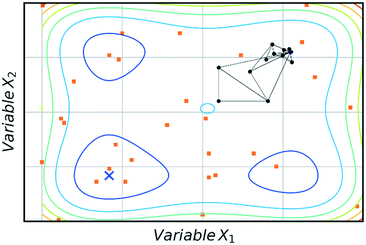Fig. 8 Comparison of SNOBFIT (orange squares) and simplex (black dots) for the minimisation of a complex function, restricted to 30 evaluations. Global minimum is indicated by a blue cross.

An alternative approach to system optimisation is to utilise kinetic model fitting. The models can then be used to suggest optimal operating conditions, provided that the kinetic equations are deconvoluted from mass transfer effects. Suggesting optimal experiments for kinetic model elucidation can be performed through model-based design of experiments. As this approach does not directly search for optimal system conditions it will not be discussed here, however, the reader is directed to the following examples should they require further information.^54–56

Multi-objective optimisation

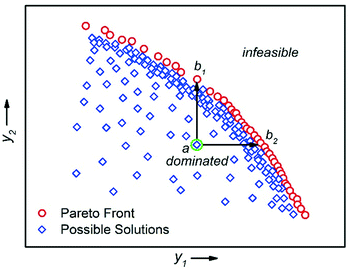
There are multiple economic and environmental process metrics that must be considered during optimisation of a chemical process.⁵⁷ These objectives are often conflicting, which means that the objective optima are located in different regions of experimental space. The optimum of each objective can be located by conducting multiple single-objective optimisations.³⁶ However, because this approach does not consider the objectives simultaneously, it fails to identify a satisfactory compromise. For example, Moore and Jensen observed a poor 42% conversion for a Paal–Knorr reaction optimised for productivity.⁴² To circumvent this, the authors repeated the optimisation using a quadratic loss function to penalise conversions lower than 85%.

The actual solution to a multi-objective optimisation problem is a set of non-dominated solutions called the Pareto front, where a non-dominated solution is one which cannot be improved without having a detrimental effect on the other.⁵⁸ Hence, a constrained multi-objective maximisation problem where variable vector x = {x₁, …, x_n} is formulated as follows. In the objective space, find variable vector x* which maximises K objective functions y(x*) = {y₁(x*), …, y_K(x*)}, where the objective space is restricted by bounds on the variables. A feasible solution a dominates another feasible solution b when y_i(a) ≥ y_i(b) for i = 1, …, K and y_j(a) > y_j(b) for at least one objective j (Fig. 9).⁵⁹

Fig. 9 An example of a multi-objective optimisation with two competing maximisation performance criteria y₁ and y₂. The Pareto front is the series of non-dominated solutions, y(x*). Solution a is dominated by all solutions between b₁ and b₂.

One approach to multi-objective optimisation is scalarisation, where objectives are combined into a single objective function with different weightings, w [eqn (1)].

This was used by Fitzpatrick et al. to simultaneously optimise throughput, conversion and consumption for an Appel reaction.³⁹ An alternative approach by Krishnadasan et al. utilised a weighted-product objective function for the optimisation of CdSe nanoparticles.⁴⁸ For both methodologies, it is difficult to define suitable weightings without substantial a priori knowledge, and minor changes to these weightings can result in significant changes to the solution obtained. Furthermore, weighting methods fail to reveal to complete trade-off in a practical number of experiments, as only one Pareto optimal solution is identified per optimisation.⁶⁰ Further work by Walker et al. utilised a constrained optimisation approach to optimise a primary objective whilst constrained within the predefined bounds applied to other objectives.⁶¹ Although this approach provides an improved means of scalarisation compared to previous work, it still fails to identify complete trade-off between objectives. In contrast, evolutionary algorithms, such as non-dominated-sort genetic algorithm (NSGA-II), are designed to converge on the Pareto front using a Pareto dominance ranking system.⁶² However, the requirement of a large population size has deterred their use in self-optimisation.

Bayesian optimisation is a broad category of derivative free (requires no gradient information) global optimisation methods that utilise surrogate models to optimise expensive-to-evaluate objective functions.⁶³ The surrogate model is built using sampled data from the process/objective to be optimised. Understanding the mechanistic concepts behind the input–output relationship is not important at this stage, with the model considered to be a ‘black box’. Once constructed, the surrogate model is utilised in conjunction with an acquisition function to suggest the next evaluation point, to maximise or minimise an objective function.⁶⁴ An acquisition function is a function which balances exploration (searching regions which currently have no data points) and exploitation (focusing near regions of known good performance) and is maximised after each iteration to determine the next sampling point. Often the surrogate model will be of the form of a Gaussian process (GP) which is computationally and resource-wise more efficient to evaluate than the actual process. A GP model is a collection of random variables, for which any discrete point has a Gaussian (normal) distribution.⁶⁵ A GP model is characterised by a mean function and a covariance function. The mean function defines the expected output for a given set of inputs, with the covariance function describing the statistical relationship between two points in the input space. Points that are close together are considered similar and this is reflected in the covariance function. A noise term can be introduced when calculating the covariance for the process. This enables Bayesian optimisation algorithms to handle noisy data associated with experimental platforms. The requirement for hyperparameters (algorithm settings) can be considered a drawback of Bayesian methodologies. The setting of these hyperparameters can play a significant role in determining the goodness of fit for the GP model and can in turn affect the performance of stochastic optimisation algorithms that use GP at their core. One example of a hyperparameter is the type of covariance function used in fitting the GP model. Fig. 10 highlights the impact of covariance function on how well the model fits the data. Ensuring hyperparameters are optimised and robust is key to developing a Bayesian optimisation algorithm. The libraries of GPy⁶⁶ and GPyOpt⁶⁷ were used for sampling and example optimisations.

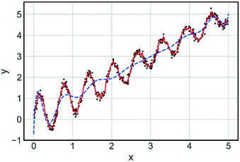Fig. 10 Comparison of fit for two Gaussian models with different covariance functions: Matern 5/2 (red) and squared exponential (blue). Training data is shown as black dots.

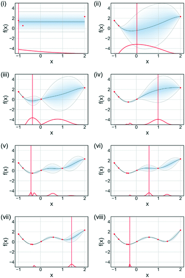
An acquisition function is used to determine the next evaluation point in Bayesian optimisation. Fig. 11 illustrates the sequential optimisation approach adopted by Bayesian optimisation techniques, with each figure representing an iteration of the algorithm. The example shown is for a single-objective problem but can be extended to multi-objective optimisations. For each iteration the acquisition function is calculated based upon the current available data and the surrogate model for the process. There are many different acquisition functions used in Bayesian optimisation tasks, with the development of acquisition functions being a constantly evolving field.⁶⁸ Some of the more common acquisition functions are expected improvement, probability of improvement, upper confidence bounds and Thompson sampling.^69,70 Mixtures of acquisition functions can also be used. Expected improvement was used for Fig. 11, with the algorithm initially exploring the search domain and then focusing on the region where the function optimum is likely to be.

Fig. 11 Bayesian optimisation (minimisation) of an arbitrary function. (i)–(viii) represent sequential iterations of the algorithm. Acquisition function is shown in red. Current estimated function is shown in blue with associated 95% confidence interval. Data is shown as red dots. The next evaluation is selected as the point which maximises the acquisition function.

The multi-objective active learner (MOAL) was designed for expensive-to-evaluate multi-target optimisation tasks.⁷¹ The algorithm was successfully applied to the optimisation of an emulsion polymerisation recipe with 14 input variables, simultaneously targeting a conversion of ≥99% and particle diameter of 100 ± 1 nm.⁷² A similar machine learning methodology was used to design the Thompson sampling efficient multi-objective optimisation (TSEMO) algorithm.⁷³ The TSEMO algorithm was shown to compare competitively with other multi-objective Bayesian optimisation algorithms such as Pareto efficient global optimisation (ParEGO)⁷⁴ and expected hypervolume improvement (EHI).⁷⁵ In addition, it can readily be used for batch-sequential design making it well suited for integration with self-optimising platforms.

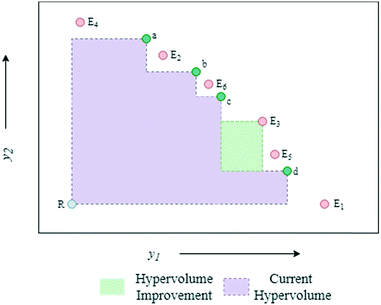
The algorithmic procedure is displayed in Fig. 12. Initially, a small dataset is collected using a random space-filling set of experiments, which is then used to build a GP surrogate model.⁷⁶ The algorithm randomly samples from the GPs and uses the NSGA-II algorithm to identify the Pareto front of each random sample (Thompson sampling). Through randomly sampling this accounts for the exploration/exploitation trade-off desirable in Bayesian optimisation. The candidate experiment which gives the largest predicted hypervolume improvement is then performed, where hypervolume is defined as the volume of objective space dominated by the current set of solutions (Fig. 13). The reference point, R, for this calculation is usually defined as the anti-utopian point (the worst point with respect to all objective functions). The hypervolume indicator is a favored metric as it considers both the convergence and diversity of the front, where diversity refers to how well-distributed the optimal solutions are along the Pareto front.⁷⁷ The combined use of random GP sampling and hypervolume improvement accounts for the desired trade-off between exploration and exploitation respectively. The GP surrogate model is then updated and the procedure repeated iteratively until the predefined maximum number of experiments is reached. Research in our group applied the TSEMO algorithm for the self-optimisation of an aromatic nucleophilic substitution (S_NAr) and N-benzylation reaction, focusing on E-factor, space–time yield (STY) and impurity profiles as objectives.⁷⁸ The algorithm was able to converge on the Pareto front in a similar number of experiments, 68 and 78 experiments respectively, as previously reported single-objective optimisations, thus providing a greater amount of information per experiment. Notably, identification of a set of solutions and presentation of a front enables a posteriori decisions to be made regarding the desired development, where process specifications are often dynamic. The inclusion of discrete variables in future work will broaden the scope of multi-objective self-optimisation to a wider variety of processes.

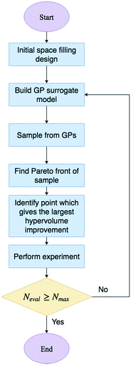Fig. 12 Flow diagram for the TSEMO algorithm. N_eval is the current number of evaluations and N_max is the maximum number of evaluations.

Fig. 13 Hypervolume plot showing the process used to select experiments from the candidate set, Ei. The current hypervolume is the volume of space dominated by the current set of non-dominated solutions (a–d). In this case, E3 is selected as it offers the largest predicted hypervolume improvement. R = reference point.

Conclusions

Combining automation with optimisation algorithms for self-optimising chemical platforms has already yielded very exciting results. Although the use of such systems are in their infancy, the drive for efficient process development and manufacturing is expected to cause this field to develop exponentially. There is a growing need to work with experts in algorithm design to: (i) further develop algorithms capable of more complex tasks, such as multi-step reaction and work-up processes; (ii) upskill non-mathematical experts such as chemists to understand when and how to use certain algorithms based on their desired outcome, such as process insight and prediction. While local methods have thus far dominated the self-optimisation literature, their simplistic nature restricts their use to problems with a single optimum. As the direction shifts to more complex chemical systems, such as multi-step reaction sequences, response surfaces will become significantly more convoluted. Hence, global and multi-objective optimisation techniques are likely to dominate over their local counterparts. As most chemical optimisations represent expensive-to-evaluate problems, improving algorithm efficiency is key in the future to minimise material consumption. The combination of surrogate models and multi-objective optimisation has recently presented an exciting opportunity to maximise the amount of useful information gained per experiment. Furthermore, the complex task of self-optimising discrete variables is likely to take precedence in future work. With this in mind, additional utilisation of techniques used heavily in computer science will prove an interesting area for the future development of self-optimising chemical platforms. We envisage that the adoption of plug-and-play self-optimising platforms will enable smarter and more efficient laboratories to flourish in the future.

Conflicts of interest

There are no conflicts to declare.

Acknowledgements

ADC, CJT and JAM thank the EPSRC and University of Leeds for funding. ADC and CJT also thank AstraZeneca for CASE student funding. This work was funded, in part, by the EPSRC project “Cognitive Chemical Manufacturing” EP/R032807/1.

References

1. M. B. Plutschack, B. Pieber, K. Gilmore and P. H. Seeberger, Chem. Rev., 2017, 117, 11796–11893.
2. S. A. May, J. Flow Chem., 2017, 7, 1–9.
3. R. L. Hartman, J. P. McMullen and K. F. Jensen, Angew. Chem., Int. Ed., 2011, 50, 7502–7519.
4. M. R. Chapman, M. H. T. Kwan, G. King, K. E. Jolley, M. Hussain, S. Hussain, I. E. Salama, C. González Nino, L. A. Thompson, M. E. Bayana, A. D. Clayton, B. N. Nguyen, N. J. Turner, N. Kapur and A. J. Blacker, Org. Process Res. Dev., 2017, 21, 1294–1301.
5. B. Gutmann, D. Cantillo and C. O. Kappe, Angew. Chem., Int. Ed., 2015, 54, 6688–6728.
6. T. Razzaq, T. N. Glasnov and C. O. Kappe, Eur. J. Org. Chem., 2009, 3, 1321–1325.
7. J. I. Yoshida, Y. Takahashi and A. Nagaki, Chem. Commun., 2013, 49, 9896–9904.
8. J. P. McMullen and K. F. Jensen, Annu. Rev. Anal. Chem., 2010, 3, 19–42.
9. R. J. Ingham, C. Battilocchio, D. E. Fitzpatrick, E. Sliwinski, J. M. Hawkins and S. V. Ley, Angew. Chem., Int. Ed., 2015, 54, 144–148.
10. A. B. Henson, P. S. Gromski and L. Cronin, ACS Cent. Sci., 2018, 4, 793–804.
11. C. Houben and A. A. Lapkin, Curr. Opin. Chem. Eng., 2015, 9, 1–7.
12. S. V. Ley, D. E. Fitzpatrick, R. J. Ingham and R. M. Myers, Angew. Chem., Int. Ed., 2015, 54, 3449–3464.
13. S. Steiner, J. Wolf, S. Glatzel, A. Andreou, J. M. Granda, G. Keenan, T. Hinkley, G. Aragon-Camarasa, P. J. Kitson, D. Angelone and L. Cronin, Science, 2019, 363, 144–152.
14. J. M. Granda, L. Donina, V. Dragone, D. L. Long and L. Cronin, Nature, 2018, 559, 377–381.
15. C. W. Coley, R. Barzilay, T. S. Jaakkola, W. H. Green and K. F. Jensen, ACS Cent. Sci., 2017, 3, 434–443.
16. C. J. Richmond, H. N. Miras, A. R. De La Oliva, H. Zang, V. Sans, L. Paramonov, C. Makatsoris, R. Inglis, E. K. Brechin, D. L. Long and L. Cronin, Nat. Chem., 2012, 4, 1037–1043.
17. D. Perera, J. W. Tucker, S. Brahmbhatt, C. J. Helal, A. Chong, W. Farrell, P. Richardson and N. W. Sach, Science, 2018, 359, 429–434.
18. B. J. Reizman and K. F. Jensen, Acc. Chem. Res., 2016, 49, 1786–1796.
19. V. Sans and L. Cronin, Chem. Soc. Rev., 2016, 45, 2032–2043.
20. D. C. Fabry, E. Sugiono and M. Rueping, React. Chem. Eng., 2016, 1, 129–133.
21. S. A. Weissman and N. G. Anderson, Org. Process Res. Dev., 2014, 19, 1605–1633.
22. R. Leardi, Anal. Chim. Acta, 2009, 652, 161–172.
23. R. Lee, Chem. Ing. Tech., 2019, 91, 191–200.
24. B. J. Reizman and K. F. Jensen, Chem. Commun., 2015, 51, 13290–13293.
25. T. E. O'Brien and G. M. Funk, Am. Stat., 2003, 57, 265–267.
26. B. J. Reizman, Y.-M. M. Wang, S. L. Buchwald and K. F. Jensen, React. Chem. Eng., 2016, 1, 658–666.
27. L. M. Baumgartner, C. W. Coley, B. J. Reizman, K. W. Gao and K. F. Jensen, React. Chem. Eng., 2018, 3, 301–311.
28. H.-W. Hsieh, C. W. Coley, L. M. Baumgartner, K. F. Jensen and R. I. Robinson, Org. Process Res. Dev., 2018, 22, 542–550.
29. A. C. Atkinson, Wiley StatsRef Stat. Ref. Online, 2015, pp. 1–17.
30. J. A. Nelder and R. Mead, Comput. J., 1965, 7, 308–313.
31. J. P. McMullen, M. T. Stone, S. L. Buchwald and K. F. Jensen, Angew. Chem., Int. Ed., 2010, 49, 7076–7080.
32. S. Krishnadasan, A. Yashina, A. J. DeMello and J. C. DeMello, in Advances in Chemical Engineering, ed. J. C. Schouten, Academic Press, 2010, pp. 195–231.
33. V. Sans, L. Porwol, V. Dragone and L. Cronin, Chem. Sci., 2015, 6, 1258–1264.
34. M. W. Routh, P. A. Swartz and M. B. Denton, Anal. Chem., 1977, 49, 1422–1428.
35. R. A. Bourne, R. A. Skilton, A. J. Parrott, D. J. Irvine and M. Poliakoff, Org. Process Res. Dev., 2011, 15, 932–938.
36. D. Cortés-Borda, K. V. Kutonova, C. Jamet, M. E. Trusova, F. Zammattio, C. Truchet, M. Rodriguez-Zubiri and F. X. F.-X. Felpin, Org. Process Res. Dev., 2016, 20, 1979–1987.
37. D. Cortés-Borda, E. Wimmer, B. Gouilleux, E. Barré, N. Oger, L. Goulamaly, L. Peault, B. Charrier, C. Truchet, P. Giraudeau, M. Rodriguez-Zubiri, E. Le Grognec and F.-X. Felpin, J. Org. Chem., 2018, 83, 14286–14299.
38. R. F. Kazmierczak Jr., DAE Research Report No. 704C61, 1997.
39. D. E. Fitzpatrick, C. Battilocchio and S. V. Ley, Org. Process Res. Dev., 2016, 20, 386–394.
40. D. Montgomery, Design and analysis of experiments, Wiley, New York, 5th edn, 2001.
41. J. P. McMullen and K. F. Jensen, Org. Process Res. Dev., 2010, 14, 1169–1176.
42. J. S. Moore and K. F. Jensen, Org. Process Res. Dev., 2012, 16, 1409–1415.
43. K. J. Beers, in Numerical Methods for Chemical Engineering: Applications in MATLAB, Cambridge University Press, New York, 2007, pp. 212–257.
44. P. Y. Papalambros and D. J. Wilde, Principles of Optimal Design, Cambridge University Press, New York, 2000.
45. R. A. Skilton, A. J. Parrott, M. W. George, M. Poliakoff and R. A. Bourne, Appl. Spectrosc., 2013, 67, 1127–1131.
46. W. Huyer and A. Neumaier, ACM Trans. Math. Softw., 2008, 35, 9.
47. N. V. Queipo, R. T. Haftka, W. Shyy, T. Goel, R. Vaidyanathan and P. K. Tucker, Prog. Aerosp. Sci., 2005, 41, 1–28.
48. S. Krishnadasan, R. J. C. Brown, A. J. DeMello and J. C. DeMello, Lab Chip, 2007, 7, 1434.
49. N. Holmes, G. R. Akien, R. J. D. Savage, C. Stanetty, I. R. Baxendale, A. J. Blacker, B. A. Taylor, R. L. Woodward, R. E. Meadows and R. A. Bourne, React. Chem. Eng., 2016, 1, 96–100.
50. N. Holmes, G. R. Akien, A. J. Blacker, R. L. Woodward, R. E. Meadows and R. A. Bourne, React. Chem. Eng., 2016, 1, 366–371.
51. N. Cherkasov, Y. Bai, A. J. Expósito and E. V. Rebrov, React. Chem. Eng., 2018, 3, 769–780.
52. M. I. Jeraal, N. Holmes, G. R. Akien and R. A. Bourne, Tetrahedron, 2018, 74, 3158–3164.
53. L. M. Rios and N. V. Sahinidis, J. Glob. Optim., 2013, 56, 1247–1293.
54. J. P. Mcmullen and K. F. Jensen, Org. Process Res. Dev., 2011, 15, 398–407.
55. S. D. Schaber, S. C. Born, K. F. Jensen and P. I. Barton, Org. Process Res. Dev., 2014, 18, 1461–1467.
56. G. Franceschini and S. Macchietto, Chem. Eng. Sci., 2008, 63, 4846–4872.
57. D. N. Jumbam, R. A. Skilton, A. J. Parrott, R. A. Bourne and M. Poliakoff, J. Flow Chem., 2012, 2, 24–27.
58. K. Deb, K. Sindhya and J. Hakanen, Decision Sciences: Theory and Practice, CRC Press, 2016.
59. A. Konak, D. W. Coit and A. E. Smith, Reliab. Eng. Syst. Saf., 2006, 91, 992–1007.
60. R. T. Marler and J. S. Arora, Struct. Multidiscipl. Optim., 2010, 41, 853–862.
61. B. E. Walker, J. H. Bannock, A. M. Nightingale and J. C. DeMello, React. Chem. Eng., 2017, 2, 785–798.
62. K. Deb, A. Pratap, S. Agarwal and T. Meyarivan, IEEE Trans. Evol. Comput., 2002, 6, 182–197.
63. E. Brochu, V. M. Cora and N. de Freitas, pre-print, 2010, arXiv:1012.2599.
64. P. I. Frazier, 2018, arXiv:1807.02811v1.
65. C. E. Rasmussen and C. K. I. Williams, in Gaussian Processes for Machine Learning, MIT Press, Cambridge, Massachusetts, 2006, pp. 7–32.
66. GPy, [Date Accessed: 12/03/18], 2012, http://github.com/SheffieldML/GPy.
67. The GPyOpt authors, [Date Accessed: 12/03/18], 2016, http://github.com/SheffieldML/GPyOpt.
68. B. Shahriari, K. Swersky, Z. Wang, R. P. Adams and N. de Freitas, Proc. IEEE, 2016, 104, 148–175.
69. J. Snoek, H. Larochelle and R. P. P. Adams, Adv. Neural. Inf. Process. Syst., 2012, 4, 2951–2959.
70. D. J. Russo, B. Roy, A. Kazerouni, I. Osband and Z. Wen, Found. Trends Mach. Learn., 2018, 11, 1–96.
71. N. Peremezhney, E. Hines, A. Lapkin and C. Connaughton, Eng. Optim., 2014, 46, 1593–1607.
72. C. Houben, N. Peremezhney, A. Zubov, J. Kosek and A. A. Lapkin, Org. Process Res. Dev., 2015, 19, 1049–1053.
73. E. Bradford, A. M. Schweidtmann and A. Lapkin, J. Glob. Optim., 2018, 71, 407–438.
74. J. Knowles, IEEE Trans. Evol. Comput., 2006, 10, 50–66.
75. M. Emmerich, Ph.D Thesis, University of Dortmund, 2005.
76. V. R. Joseph and Y. Huang, Stat. Sin., 2008, 18, 171–186.
77. A. Auger, J. Bader, D. Brockhoff and E. Zitzler, Theor. Comput. Sci., 2012, 425, 75–103.
78. A. M. Schweidtmann, A. D. Clayton, N. Holmes, E. Bradford, R. A. Bourne and A. A. Lapkin, Chem. Eng. J., 2018, 352, 277–282.

---

Footnote

† These authors contributed equally to the preparation of the manuscript.

---