
 Open Access Article
 This Open Access Article is licensed under a
 Creative Commons Attribution 3.0 Unported Licence
An improved liquid–liquid separator based on an optically monitored porous capillary†
Andrew J.
Harvie
 a,
Jack O.
Herrington
b and
John C.
deMello
*a
a,
Jack O.
Herrington
b and
John C.
deMello
*a
aDepartment of Chemistry, Norwegian University of Science and Technology, Trondheim, Norway. E-mail: john.demello@ntnu.no
bFaculty of Engineering, Department of Bioengineering, Imperial College London, London, UK
First published on 3rd June 2019
Abstract
We report an easily assembled, high performance liquid/liquid separator constructed from a drilled-out block of aluminium, a short length of porous polytetrafluoroethylene tubing, and a small number of off-the-shelf components and 3D-printed parts. The separator relies on the two incoming liquids having different wettabilities to the wall of the porous capillary, with the more strongly wetting liquid leeching through the porous wall while the other liquid passes unhindered through the interior channel. To achieve complete separation of the two phases, the fluid streams at the separator outlets are monitored optically, and the back-pressure at one outlet is iteratively adjusted using a motorised needle valve until smooth time-invariant signals are recorded at both outlets. The separator may be applied to many pairings of immiscible liquids over a broad range of flow rates, automatically establishing complete separation within minutes of activation and adjusting dynamically to subsequent changes in the flow conditions. The separator – whose performance is competitive with far costlier commercial systems – is released here as open hardware, with technical diagrams, a full parts list, assembly instructions, and source code for its firmware.
Introduction
Separating intimate mixtures of immiscible liquids into continuous streams of their constituent liquids is a critical process in flow-based chemistry.1 Key applications of liquid–liquid separation include: (i) multistep chemistry,2,3 where it may be necessary to switch repeatedly between segmented flow and single-phase flow to carry out different steps of a reaction; (ii) inline analysis,4 where moving from a segmented flow to a single-phase flow can simplify detection; and (iii) purification,5,6 where it is necessary to separate a target molecule (in one solvent) from impurities (in the other) following liquid–liquid extraction.Phase separation in microscale systems is most effectively achieved using wetting-based methods that exploit differences in the tendencies of the constituent liquids to wet a surface or membrane. One approach is to use micro-engineered structures to induce phase separation and coerce the two liquids into following separate exit paths (as a result of one liquid maximizing and the other liquid minimizing its contact with an exposed surface).7–15 Another approach, exploited in some commercial systems, is to use porous, planar membranes that are selectively permeated by one of the two phases.16–21
In previous work4,6,22 we reported an alternative method for separating immiscible liquids, using a commercially sourced porous polytetrafluoroethylene (PTFE) capillary, see Fig. 1a. Injection of a two-phase flow into the porous capillary causes one phase – the wetting phase – to preferentially permeate the capillary wall, leaving a continuous stream of the other phase – the non-wetting phase – to emerge from the end of the capillary (the “through-outlet”, T). If the porous capillary is encased in an outer jacket, the wetting-phase may also be coerced into a continuous stream and extracted at a second outlet (the “side-outlet”, S). In this way, continuous separated streams of the two phases may be readily obtained over a broad range of flow conditions using a wide variety of liquid–liquid combinations, including aqueous–organic, aqueous–fluorous and organic–fluorous mixtures.6
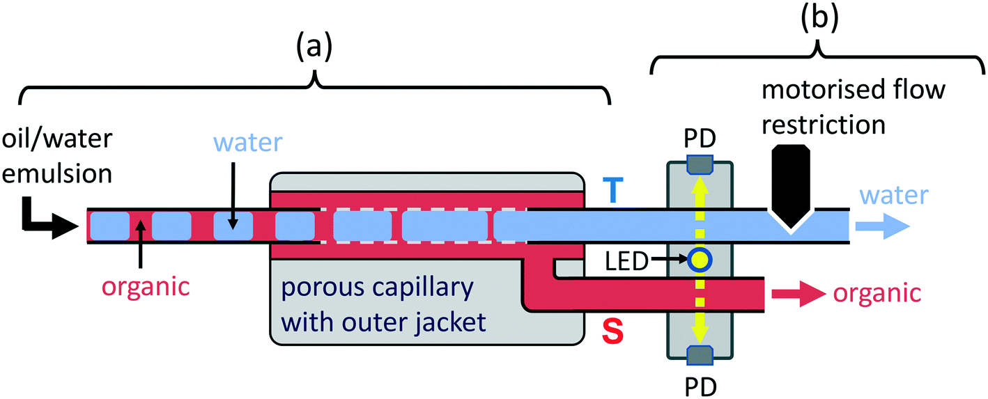 | ||
| Fig. 1 Principle of capillary-based liquid–liquid separation. (a) The segmented flow is passed into a short length of porous PTFE tubing, causing the wetting liquid to preferentially pass through the capillary wall into a jacket surrounding the capillary, where it is coerced into a continuous stream and extracted via a side-channel (S); the non-wetting liquid passes through the porous capillary unaffected and emerges as a continuous stream via the through-channel (T); (b) automation is achieved by monitoring each outgoing fluid stream with a constant intensity light-emitting diode (LED) and a photodetector (PD), and iteratively adjusting a motorised needle-valve at T until smooth non-fluctuating signals are obtained at both outlets. | ||
To achieve complete separation of the two liquids, the back-pressures at T and S must be carefully controlled: if, for instance, the back-pressure at T is too high, a fraction of the non-wetting liquid will be forced through the capillary wall, leading to its incomplete recovery at T; if it is too low, a fraction of the wetting liquid will pass through the entire length of the porous tubing without being depleted through the wall, causing a mixture of the two liquids to emerge at T. Hence, to achieve complete separation, a flow restriction must be placed at the under-pressured outlet to establish an appropriate pressure differential between the two outlets. The correct choice of flow restriction depends on many factors, including the viscosities, densities and interfacial tensions of the liquids in the incoming flow and the fluidic resistance of the flow components downstream of the separator outlets (which are affected in turn by the flow rates of the incoming liquids). Hence, to achieve complete separation, the flow restriction must be carefully matched to the specific liquids and conditions employed.
It follows that a fixed flow restriction will be effective only over a limited range of flow conditions (outside of which imperfect separation will occur). In a recent paper,22 we showed that complete liquid/liquid separation may be achieved over a much wider range of flow rates by using a needle valve coupled to a stepper motor to dynamically vary the flow resistance at the under-pressured outlet, see Fig. 1b. The correct setting of the valve was determined by monitoring the optical transmittance of the fluid streams at the two outlets (using amplified photodiodes), and iteratively modifying the valve position until smooth time-invariant signals were observed at both outlets. In this way, we obtained a fully automated separator that could induce complete separation within minutes without manual intervention. In this paper, we propose several design modifications to reduce construction costs, simplify assembly, and improve the performance of the automated separator, thereby elevating it from a proof-of-principle prototype to a reliable and practical tool for flow chemistry.
Mechanical design
The most significant design change is the integration of the jacketed separator into a single block of machined aluminium (see Fig. 2 and S1†) – a substantial simplification compared to our previous modular design.22 The machined block serves several roles: it houses the porous capillary, it provides a jacketing void-space around the porous capillary for collection of the wetting phase, and it provides (three) tapped holes to accommodate nut-and-ferrule-style fluidic connections to the outside world. One connection is used to couple (non-porous) exterior tubing at the inlet to the rear-end of the porous capillary; another is used to couple exterior tubing at the T-channel outlet to the front-end of the porous capillary; while the other is used to couple exterior tubing at the S-channel outlet to the exit port of the jacket‡ (please refer to the ESI† for full fabrication and assembly details). Using a monolithic housing for the porous capillary offers several advantages over our previous modular design, including a substantially reduced component count, easier and quicker assembly, a smaller spatial footprint, and improved ease of use; it has also allowed us to reduce the jacketing volume around the porous capillary to ∼120 μL (down from ∼210 μL in our previous modular design), decreasing the space available for problematic trapping of gas bubbles or liquid droplets – an occasional cause of separator misbehaviour.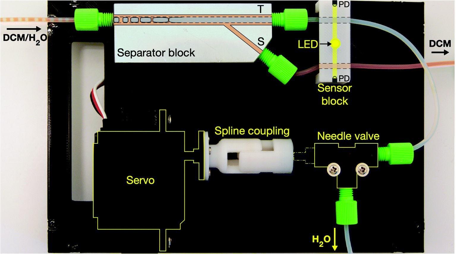 | ||
| Fig. 2 Annotated photograph of automated separator in T-mode configuration, comprising a machined aluminium separator block for inducing phase separation, a sensor block containing an LED and two photodetectors (PDs) for optically monitoring the two output channels of the separator, and a motorised needle valve for controlling the back-pressure at the T-channel outlet. Note, DCM has been dyed with Sudan orange. | ||
In addition to modifying the housing for the porous capillary, we have also made several changes to the exterior componentry, with a view to further simplifying the design, reducing build costs, and improving reliability and ease of use. The most notable changes are: the replacement of a desktop personal computer (PC) by a microcontroller (μC); the replacement of the stepper motor by a positional servo (motor); and the replacement of the amplified photodiodes by light-to-frequency (LTF) converters. The transfer of programmatic control from a desktop PC to a microcontroller allows the new separator to operate in a fully autonomous manner without the need for connection to a PC or other hardware. The use of a multi-turn positional servo – whose angular position is straightforwardly controlled by a pulse-width-modulation (PWM) signal from a digital output pin of the microcontroller – eliminates the need for a separate motor driver and allows for easy homing of the valve (to its closed position) at the start of a run without external feedback sensors. And the use of (digital) LTF converters in place of (analogue) amplified photodiodes provides better resilience to electrical inference from mechanised laboratory equipment, increasing reliability. It also permits – if so desired – the use of extremely low cost microcontrollers that lack analogue-to-digital-conversion capabilities.
The automated separator comprises three discrete parts mounted on a common 3D-printed base-plate (see Fig. 2 and S2 and S3†): a separator block (described above), a sensor block for optically monitoring the outlet channels, and a motorised needle valve for controlling the back-pressure at the under-pressured outlet. The sensor block is a structured piece of opaque plastic, containing two parallel holes through which the outlet tubing from the T- and S- channels are separately threaded, plus a third orthogonal through-hole that allows light to pass through the two channels (see Fig. S4†). A single light-emitting diode (LED) in the centre of the orthogonal through-hole is used to illuminate both pieces of tubing; and two light-to-frequency converters located at opposing ends of the orthogonal through-hole are used to detect light transmitted through the tubing. For convenience, we have integrated the sensor block directly into the baseplate, allowing the combined base-plate/sensor-block to be fabricated in a single print run.
The motorised valve comprises a positional servo, an off-the-shelf needle valve, and a simple home-made spline coupling for transmitting torque between the servo and the screw-head of the needle valve. The spline coupling is formed from two interlocking halves that are free to slide across one another along the axis of rotation (see Fig. 2 and ESI†), allowing the coupling to adjust smoothly to the displacement of the screw-head as it rotates. Fluidic connections to the needle-valve are made using two additional nut-and-ferrule connectors. Integrated fixtures in the base-plate allow for easy alignment and mounting of the motorised valve. A circuit diagram for the complete system is provided in Fig. S5.†
The full parts list is quite short, comprising the machined separator block, a 60 mm section of commercially sourced porous PTFE tubing, standard (non-porous) PTFE tubing, five nut-and-ferrule connectors, an off-the-shelf needle-valve, a positional servo, a light-emitting diode, two LTF converters, a simple microcontroller, and a low voltage DC power supply or battery. The separator is intended to be used as a stand-alone system, but the μC may optionally be connected to a PC (via a serial interface) for data storage and visualisation purposes. Manual assembly of the entire system is straightforward and, with parts to hand, may be accomplished in less than thirty minutes. The trickiest aspect of assembly is attachment of the porous capillary to the fluidic connectors, but detailed instructions are provided in the ESI.† Owing to the simplicity of the design and the low component count, the entire system can be put together for less than £100 on a one-off basis (and for much less when ordering parts in bulk).
Optimisation routine
The motor movement is controlled using a simplified version of the algorithm reported in ref. 22. For the purpose of explanation, we will suppose the separator is in use, with a two-phase fluid stream entering its inlet and the motorised valve located at the T-channel outlet (as in Fig. 2). If the liquid/liquid separation is perfect and a single phase is flowing uniformly through each exit channel, the T- and S-channel photodetectors will both generate stable, time-invariant signals. On the other hand, if the separation is imperfect, at least one of the photodetectors will generate a fluctuating signal due to differential absorption or scattering of incident light by the two-phase flow (scattering is caused by the different refractive indices of the two liquids, and so will occur even with colourless solutions).The signal fluctuations in the S- and T-channels may be conveniently quantified in terms of their relative standard deviations (RSD's), γS and γT (note, the RSD γ of a signal is obtained by dividing its standard deviation σ by its mean μ: γ = σ/μ; a high RSD therefore indicates a highly fluctuating signal and vice versa). Assuming the chosen liquid/liquid combination is separable, four scenarios may occur: (i) the RSD may be high in the S-channel and low in the T-channel, indicating both liquids are passing through the wall of the porous capillary and the valve (at T) should be loosened; (ii) the RSD may be low in the S-channel and high in the T-channel, indicating both liquids are passing straight through the porous capillary and the valve should be tightened; (iii) the RSD may be low in both channels, indicating good separation; or (iv) the RSD may be moderately high in both channels, indicating the valve is close to being in an acceptable position but still requires some further tuning and/or stabilisation to achieve complete separation.
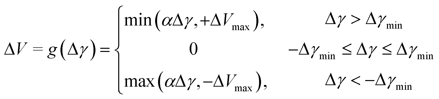
In practice, there is a relatively broad window of valve positions that will give complete separation, which we refer to as the “separation window”. The direction of valve rotation needed to reach the separation window from a given starting position may be readily identified by subtracting the RSD value of the T-channel from the RSD value of the S-channel to obtain a differential RSD Δγ = γS − γT. If Δγ is large and positive, too much liquid is passing through the wall of the porous capillary and the valve (at T) should be opened to reduce the back-pressure at the end of the capillary; conversely, if Δγ is large and negative, too much liquid is passing straight through the porous capillary and the valve should be tightened. High values of |Δγ| occur when the valve position is far from the separation window, meaning a large angular rotation is required to bring the system into a state of complete separation. Close to the separation window |Δγ| is smaller and a smaller angular rotation is required. This suggests the use of a simple iterative algorithm, in which the angular rotation ΔV made within a single iteration scales linearly with Δγ such that ΔV = αΔγ, where α is a user-defined proportionality constant. In practice we find it is beneficial to make two modifications to this general approach: firstly, we cap the maximum rotation at a value ΔVmax to avoid repeated overshooting of the separation window; and, secondly, we suppress valve movements when the magnitude of the differential RSD is smaller than a threshold value Δγmin to avoid ‘twitching’ of the valve position when the valve is already inside the separation window. The valve adjustment ΔV for a given differential RSD value Δγ is therefore given by the following equation:
 | (1) |
(Note, this is a simpler expression than the one we reported in ref. 22, requiring the specification of fewer user-defined parameters). Δγmin is typically set to be slightly higher than the differential RSD measured when both channels are empty, i.e. when no liquid is present in the system (and any fluctuations in the signals are therefore due to intrinsic noise in the detection system); ΔVmax is typically set to a small fraction of a full turn (here 80°); while α – which determines how aggressively the valve responds to the measured differential RSD values – is chosen empirically to give rapid convergence without ‘ringing’ of the valve position (see ESI†). Once suitable values for Δγmin, ΔVmax and α have been identified for one liquid/liquid combination and flow rate, they can typically be applied without adjustment to many other liquid/liquid combinations and flow conditions.
The optimisation routine begins with the valve set to the closed position, and all subsequent valve movements are then made in accordance with eqn (1). To ensure fast convergence, it is necessary in each iteration to update the valve position before the system has reached steady-state in the expectation that repeated adjustments will quickly bring the system into a state of complete separation (despite individual measurements being made prematurely). For all of the data reported below, a wait-time (td) of two seconds was imposed after setting each new valve position (to allow time for the valve to move to its new position and for the flow to partially stabilise); four seconds' worth of data was then acquired concurrently from each channel at a sample-rate of 50 Hz; and a new valve position was then set immediately using eqn (1) before commencing the next iteration. The total time between each iteration (i.e. between the start of each valve adjustment) was therefore 6 s.
The optimisation routine continues to run even after complete separation has been achieved. Hence, in the event of an external disturbance that disrupts the separation, the optimisation routine makes whatever adjustments are needed from the current valve position V to restore the separation. (There is no need to wind the valve back to the zero position and start again). Importantly, the optimisation procedure is robust against occasional anomalies (“blips”) in the measured signals due e.g. to gas bubbles passing through one of the detection zones: minor blips are ignored due to the minimum threshold for |Δγ|, while larger blips cause only a momentary adjustment to the valve position that is rapidly corrected once the anomaly has passed.§
The complete logic flow of the algorithm is summarised in Fig. 3. All measurements reported below were obtained using the formulation described in the flow chart with the parameter values summarised in the adjacent table.
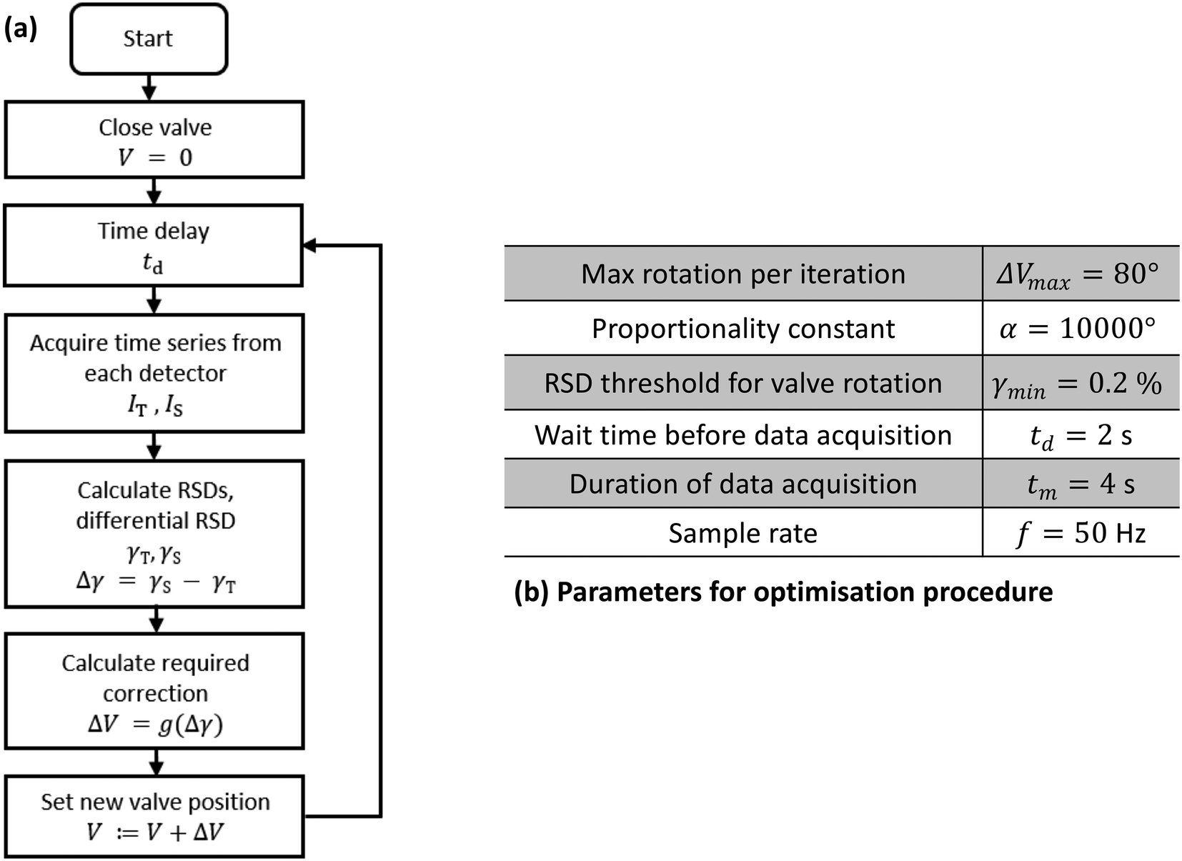 | ||
| Fig. 3 Details of optimisation procedure: (a) Flow chart summarising the automated procedure used to bring the system into a state of complete separation: (i) the valve is closed and variables are initialized; (ii) a two-second delay is imposed; (iii) four-second traces are recorded at the T- and S-channel outlets, and quantified in terms of their respective RSD values, γT and γS; (iv) the required adjustment ΔV of the valve position is determined from Δγ = γS − γT, using eqn (1); (iv) variables are updated and steps (ii), (iii) and (iv) are repeated until the end of the run. (b) Table of parameters used for optimisation procedure. | ||
Results
Evaluation of separator with an under-pressured T-channel (“T-mode” operation)
The need for the wetting phase to pass through the micron-scale pores of the porous capillary often results in a substantially higher back-pressure at S than T, meaning the T-channel outlet is commonly the under-pressured outlet where the needle-valve must be placed (see Fig. 4a and S6b†). We refer to this setup – in which the T-channel is the actively controlled channel containing the valve and the S-channel is the passive channel with no flow control – as the “T-mode” of operation. | ||
| Fig. 4 Photographs showing the two operating modes for the separator, achieved via a simple reconfiguration of the outlet tubing. The motorised valve is always connected to the under-pressured outlet, so the T-mode configuration (a) is used when the T-channel is under-pressured, and the S-mode configuration (b) is used when the S-channel is under-pressured. Note, DCM in S-channel has been dyed with Sudan orange. | ||
To evaluate the T-mode performance of the separator, a segmented flow of dichloromethane (DCM) and water was used as a test system. DCM has the stronger affinity for PTFE and is therefore the wetting-phase to be extracted through the S-channel outlet, while water is the non-wetting phase to be extracted through the T-channel outlet (note, the terms “wetting” and “non-wetting” are intended to be relative rather than absolute). The segmented flow was generated by injecting each liquid into a separate input of a “two-in/one-out” PTFE droplet generator at a flow-rate of 300 μL min−1 (see Fig. S7†), corresponding to a total incoming flow-rate of 600 μL min−1. The outlet of the droplet generator was connected to the inlet of the separator block by a short length of (non-porous) PTFE tubing.
Fig. 5a shows illustrative 4 s-traces for the T- and S-channel signals at different stages of the optimisation run, while Fig. 5b shows the differential RSD (blue line) and angular position (red line) versus time. At the start of the optimisation run (iteration zero), the valve is set to the fully closed position (V = 0) – forcing the entire two-phase fluid stream to pass through the side-channel – which leads to a broadly static signal at T (red line) and a strongly fluctuating signal at S (blue line) (the static nature of the T signal reflects the absence of liquid flow in the (closed) through-channel, while the irregular appearance of the S signal is characteristic of a disordered two-phase flow, in which alternating slugs of the two liquids are constantly crossing the detection zone). In consequence, a large positive differential RSD value of approximately five percent is obtained which, for the optimisation parameters chosen, results in the maximum permissible positive valve rotation of +80°. The RSD value is largely unchanged at the next iteration (1), leading to another rotation of +80°. It is only after the seventh successive +80°-valve-shift (start of iteration 7) that the situation changes appreciably, with the fluctuations in the S-channel disappearing except for a single prominent feature at ∼3.8 s. This behaviour indicates that the majority of the liquid passing out of the S-channel is now DCM (the wetting phase), with only a small amount of (unwanted) water leaking through. The change in the appearance of the S-channel trace leads to an approximate five-fold reduction in the differential RSD to 1% but, for the chosen proportionality constant (α = 10![[thin space (1/6-em)]](https://www.rsc.org/images/entities/char_2009.gif) 000°), this still results in the maximum permitted valve shift of +80°. By the start of the next iteration (8) the system is already close to complete separation, with only occasional minor blips in the S-channel signal due to occasional water leakage through the porous capillary wall, resulting in a differential RSD of 0.25%. A further adjustment of +24° brings the system into complete separation with smooth signals in both channels and a differential RSD value of 0.001%, which is too small to elicit any rotation of the valve. The valve position remains fixed for the remainder of the run, with smooth signals continuing to be observed in both channels, consistent with complete separation from then on. Complete separation was confirmed by comparing the (g min−1) mass collection rate at each outlet to the mass injection rate of liquid from the corresponding syringe, with the T- and S-channel outlets matching the respective injection rates for water and DCM to within experimental error (1%), see Fig. S8a.†
000°), this still results in the maximum permitted valve shift of +80°. By the start of the next iteration (8) the system is already close to complete separation, with only occasional minor blips in the S-channel signal due to occasional water leakage through the porous capillary wall, resulting in a differential RSD of 0.25%. A further adjustment of +24° brings the system into complete separation with smooth signals in both channels and a differential RSD value of 0.001%, which is too small to elicit any rotation of the valve. The valve position remains fixed for the remainder of the run, with smooth signals continuing to be observed in both channels, consistent with complete separation from then on. Complete separation was confirmed by comparing the (g min−1) mass collection rate at each outlet to the mass injection rate of liquid from the corresponding syringe, with the T- and S-channel outlets matching the respective injection rates for water and DCM to within experimental error (1%), see Fig. S8a.†
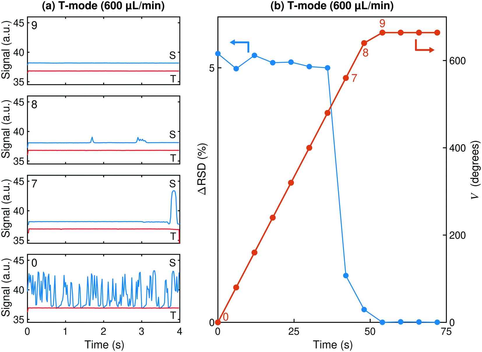 | ||
| Fig. 5 T-mode behaviour of automated separator, using equal flow rates of 300 μL min−1 for water and DCM. (a) Plots showing four-second traces recorded in the T-channel (red lines) and S-channel (blue lines) at key stages of the optimisation run. (b) Plot showing valve position V (red line, b) and differential RSD value Δγ (blue line, b) versus time. Starting from an initial position of V = 0° (in which the entire two-phase fluid stream was forced through S), a series of seven large, positive Δγ values of approximately five percent were obtained at the start of the run due to strong fluctuations in the S-channel, causing the valve to make seven sequential positive adjustments at the maximum allowed adjustment of ΔV = +80°. Δγ fell to one percent at the seventh iteration, with a broadly flat signal in the S-channel except for a single large ‘blip’ at ∼3.8 s, resulting in another adjustment of ΔV = +80° and further reducing Δγ to 0.25%. One further adjustment of ΔV = +24° brought the system into complete separation (Δγ < 0.01%), with the valve position fixed at V = 664° thereafter. | ||
Fig. 6a shows the T-mode performance of the automated separator at different total flow rates in the range 100 to 4800 μL min−1, using equal injection rates of water and DCM. Convergence was rapid in all cases, with complete separation being achieved in less than two minutes (and in less than one minute for flow rates of 600 μL min−1 and above). At the highest flow rate of 4800 μL min−1 the separator exhibits a very simple position-time curve, in which the valve position increments steadily at the maximum rate of 80° per iteration for the first six iterations. It then executes one further adjustment of ΔV = +72°, bringing the system into a state of complete separation at V = 452°. As the flow rate is reduced, however, the position-time curves become increasingly ‘stepped’ in appearance due to the valve position freezing during some iterations. This behaviour is attributable to the segmentation of the liquid/liquid flow which – for long slugs and/or slow flow rates – can lead to anomalously low differential RSD values (below the threshold for valve movement) as a result of only a single liquid crossing the S-channel sensor during the data acquisition period. The intermittent freezing of the valve position accounts for the increased convergence time at low flow rates and could, if necessary, be mitigated by increasing the acquisition period (at the expense of an increased time per iteration).
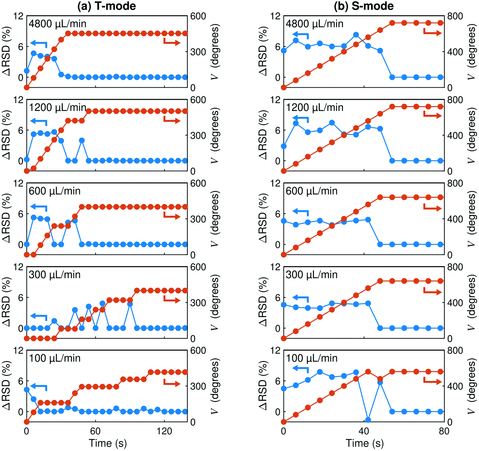 | ||
| Fig. 6 Performance of automated separator under various flow rates, using equal injection rates of water and DCM. Each plot shows for a different total flow rate the valve position V (red line) and the differential RSD Δγ (blue line) versus time, starting from an initial position of V = 0°. The left (a) and right (b) plots show the behaviour of the separator in T- and S- mode operation, respectively. In all cases, convergence to a state of complete separation is achieved in less than two minutes. The ‘stepping’ of the T-mode position-time plots is due to a single slug of liquid crossing the S-channel sensor during some iterations, resulting in an anomalously low differential RSD that is below the threshold for valve movement; this effect is most pronounced at low flow rates due to the slow passage of liquid across the S-channel sensor. | ||
The results in Fig. 6a were obtained using equal flow rates for water and DCM, but the separator may also be applied in situations where the flow rates are imbalanced. In Fig. S9a,† we show T-mode data for a series of runs using H2O:DCM flow-rate ratios in the range 1:10 to 10:1, keeping the total flow rate fixed at 1000 μL min−1. The separator was able to rapidly induce complete separation in all cases, with convergence being achieved in 96 s or less.
Evaluation of separator with an under-pressured S-channel (“S-mode” operation)
In some fluidic set-ups – e.g. those in which there are resistive flow components downstream of the T-channel outlet – the S-channel may be the under-pressured outlet where active flow control is required. To address the under-pressure at S, the variable flow resistance is moved to S via a simple reconfiguration of the separator block's outlet tubing (“S-mode” operation, see Fig. 4b and S6b†), and the differential RSD is redefined as Δγ = γT − γS (to ensure the valve opens when the T-channel fluctuations are stronger than the S-channel fluctuations). No other changes are required to the experimental set up or to the optimisation routine.Fig. 6b shows the S-mode behaviour of the separator at flow rates in the range 100 to 4800 μL min−1, where the S-channel outlet has been forced into an under-pressured state by subjecting the T-channel tubing to a 25° bend, see Fig. S6a.† As before, each run begins with the valve fully closed, which in this case causes the entire two-phase fluid stream to pass through the T-channel. In all cases convergence is obtained within one minute, with the valve position incrementing steadily at the maximum rate of 80° per iteration until the separation window is reached (and the differential RSD falls below the threshold needed for further valve movement). The only slight deviation from this behaviour is observed at the lowest flow-rate of 100 μL min−1, where there is a brief tightening of the valve (ΔV = −80°) at iteration seven, followed by a loosening of the valve at iteration eight (ΔV = +80°) to bring the system into final convergence at V = 560°. (Inspection of the T- and S-channel traces reveals this ‘glitch’ to be caused by a momentary escape of DCM or trapped air from the separator during iteration seven, see Fig. S10†).
It is notable that the S-mode behaviour at all flow rates closely resembles the T-mode behaviour of the separator at the highest flow-rate of 4800 μL min−1, with none of the step-like features evident in T-mode at lower flow rates, resulting in fast sub-minute convergence for all flow rates investigated. This, however, is not always the case and step-like behaviour is sometimes observed in S-mode operation too (especially when high back-pressures are present on the T-channel, see e.g.Fig. 7c).
 | ||
| Fig. 7 Response of automated separator to abrupt changes in flow rate, using equal injection rates of water and DCM. Each plot shows for a different flow configuration the valve position V (red line) and the differential RSD Δγ (blue line) versus time, starting from an initial position of V = 0° at a flow rate of 100 μL min−1, with an increase to 4800 μL min−1 at t = 456 s and a decrease back to 100 μL min−1 at t = 1200 s. The upper (a) and middle (b) plots show the T-mode behaviour of the separator without (T-mode) and with (T-mode II) flow restrictions on the S- and T-channels, while the lower plot (c) shows the S-mode behaviour of the separator (with high back-pressure on the T channel). In the case of T-mode operation without added back-pressure, no change in valve position is required to maintain separation due to the broad separation window of the system. For T-mode II and S-mode operation, changes in flow rate cause short-lived deviations from perfect separation that are rapidly compensated by adjustments of the valve position, with complete separation being restored within two minutes. | ||
Complete separation was again confirmed by comparing the (g min−1) mass collection rate at each outlet to the mass injection rate of liquid from the corresponding syringe, with the T- and S-channel outlets matching the respective injection rates for water and DCM to within experimental error (1%), see Fig. S8b.†
The S-mode performance of the separator was also assessed using imbalanced H2O:DCM flow-rate ratios in the range 1:10 to 10:1, keeping the total flow rate fixed at 1000 μL min−1 as before (see Fig. S9b†). The separator was able to rapidly induce complete separation in all cases, with convergence being achieved in 126 s or less.
Transient response of separator under T- and S-mode operation
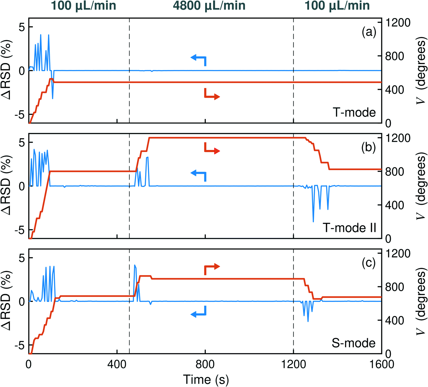
Lastly, we turn to the question of how the separator responds to sudden changes in the flow conditions. We note from Fig. 6 that, in both modes of operation, there is a weak shift towards higher final valve positions as the flow rate is increased. In the case of T-mode operation, the valve position increases from V = 416° at 100 μL min−1 to V = 452° at 4800 μL min−1, while for S-mode operation it increases from V = 560° to V = 720°. This suggests that in both cases the fluidic resistance of the active channel (including the needle valve) increases more rapidly with flow rate than the fluidic resistance of the passive channel, necessitating an opening of the valve to reduce the active channel pressure and thus restore separation. We note, however, that for any given flow rate there is a rather broad range of valve positions over which the separator block is capable of inducing complete separation; consequently, significant changes in flow rate can often be accommodated without requiring any change in valve position.The ability of the separator to maintain separation after a change of flow rate can be seen for example in Fig. 7a, which shows the T-mode behaviour of the separator over a thirty minute run where the flow rate of the incoming liquid stream was initially set to 100 μL min−1 at time t = 0 s, then (abruptly) increased to 4800 μL min−1 at t = 456 s, and then (abruptly) reduced back to 100 μL min−1 at t = 1200 s, using the same T-mode set up as before. The initial behaviour matches that seen previously in Fig. 6a, with the separator showing a stepped position-time profile due to alternation of the differential RSD between large and small values (depending on the nature of the liquid flow crossing the S-channel sensor during a given iteration). Once convergence is reached at t = 114 s, complete separation is maintained for the rest of the run, with no further changes in valve position despite the large flow rate changes at t = 456 s and t = 1200 s. Close inspection of the differential RSD values in the 60 s before and after the flow rate changes reveals no appreciable change in value, confirming the maintenance of complete separation.
In circumstances where there is high back-pressure at one or both outlets, the location of the separation window becomes much more sensitive to the flow rate, and significant adjustments in the valve position are required to maintain separation. This can be seen in Fig. 7b, which shows the behaviour of the separator under equivalent flow conditions to Fig. 7a but with a fixed flow restriction now placed on the S- and T-channel outlets, see Fig. S6b† (we refer to this setup as T-mode II). Complete convergence is attained within 96 s, after which the system remains in a state of complete separation until the flow rate is increased to 4800 μL min−1 at t = 456 s, causing an increase in the differential RSD at t = 486 s, which leads to a series of valve adjustments until complete separation is restored at t = 546 s.
We noted earlier that there is broad shift to higher (more open) final valve positions as the flow rate is increased. The trend is much stronger when there is significant back-pressure on the two outlet channels. The effect of increasing the flow rate at t = 456 s is therefore to substantially over-pressure the T-channel outlet, which forces a fraction of the (non-wetting) water to leak through the wall of the porous capillary alongside the DCM. The resulting fluctuations in the S-channel signal yield a series of positive differential RSD values, which cause a progressive opening of the valve over the next ten iterations until complete separation is restored 90 s after the change of flow rate (at V = 1200°). The system remains in a state of complete separation until t = 1200 s when the flow rate is reduced back to 100 μL min−1. For the reasons just discussed, the effect of lowering the flow rate is to under-pressure the T-channel outlet, which allows a fraction of the (wetting) DCM to leak through the T-channel outlet. The resulting fluctuations in the T-channel signal yield a series of negative differential RSD values, which cause a progressive tightening of the valve over the next eighteen iterations, with complete separation being restored at t = 1362 s (i.e. 162 s after the second change of flow rate). The new valve position (V = 824°) closely matches the original (converged) valve position (V = 800°), and the system remains in a state of complete separation for the remainder of the run.
In S-mode operation (with a flow restriction at T) the behaviour is broadly the same (see Fig. 7c), with convergence times of 100 and 132 s for the 100–4800 and 4800–100 μL min−1 transitions, respectively. There is a slight overshoot of the valve position for both transitions, which are corrected by single valve shifts of ΔV = −34° and ΔV = +22° at t = 558 s and 1332 s, respectively. Hence, even with high back-pressures at the outlets, the separator is able to respond dynamically to changes in flow rate in both T- and S-mode operation, successfully restoring complete separation within three minutes. We note the existence of substantial time lags between changing the flow rates and the valve responding, which are attributable to the dead volume in the separator and associated tubing: as expected, the time lags are shorter for the low-to-high transitions (∼30 s) than for the high-to-low transitions (∼60 s) due to the higher post-transition flow-rate in the former case, which has the effect of sweeping out the dead-volume more quickly.
Conclusion
In summary, we have reported a high performance liquid/liquid separator constructed from a drilled-out block of aluminium, a short length of porous polytetrafluoroethylene tubing, and a small number of off-the-shelf components and 3D-printed parts. The new separator is an improvement on the modular device we reported last year, with a number of design modifications to reduce construction costs, simplify assembly, and increase performance and reliability. The most significant design change is the integration of the jacketed separator into a single block of machined aluminium, reducing the parts count and simplifying assembly. Importantly, the new separator has a substantially reduced jacket-volume compared to our previous design, and is consequently less prone to unwanted trapping of fluids (whose intermittent and uncontrolled release can lead to occasional, spurious valve movements). Other changes include the use of a microcontroller for autonomous stand-alone operation, and the use of a positional servo for easier valve control. The separator may be applied to many liquid/liquid combinations¶ over a broad range of flow rates, achieving complete separation within minutes of activation, and is able to maintain (or rapidly restore) separation even after large changes of flow rate. The simple construction of the separator and its ease of use, low cost, and very competitive performance characteristics make it a promising tool for flow chemistry. The separator is released here as open hardware, with technical diagrams, a full parts list, assembly instructions, and source code for its firmware included in the ESI.†Conflicts of interest
There are no conflicts to declare.References
- C. Xu and T. Xie, Ind. Eng. Chem. Res., 2017, 56, 7593–7622 CrossRef CAS.
- T. Noël, S. Kuhn, A. J. Musacchio, K. F. Jensen and S. L. Buchwald, Angew. Chem., Int. Ed., 2011, 50, 5943–5946 CrossRef.
- A. M. Nightingale, T. W. Phillips, J. H. Bannock and J. C. de Mello, Nat. Commun., 2014, 5, 3777 CrossRef CAS PubMed.
- J. H. Bannock, T. W. Phillips, A. M. Nightingale and J. C. deMello, Anal. Methods, 2013, 5, 4991 RSC.
- N. Weeranoppanant, A. Adamo, G. Saparbaiuly, E. Rose, C. Fleury, B. Schenkel and K. F. Jensen, Ind. Eng. Chem. Res., 2017, 56, 4095–4103 CrossRef CAS.
- T. W. Phillips, J. H. Bannock and J. C. deMello, Lab Chip, 2015, 15, 2960–2967 RSC.
- A. Günther, M. Jhunjhunwala, M. Thalmann, M. A. Schmidt and K. F. Jensen, Langmuir, 2005, 21, 1547–1555 CrossRef PubMed.
- E. Kolehmainen and I. Turunen, Chem. Eng. Process.: Process Intesif., 2007, 46, 834–839 CrossRef CAS.
- M. N. Kashid, Y. M. Harshe and D. W. Agar, Ind. Eng. Chem. Res., 2007, 46, 8420–8430 CrossRef CAS.
- O. K. Castell, C. J. Allender and D. A. Barrow, Lab Chip, 2009, 9, 388–396 RSC.
- F. Scheiff, M. Mendorf, D. Agar, N. Reis and M. Mackley, Lab Chip, 2011, 11, 1022 RSC.
- W. A. Gaakeer, M. H. J. M. de Croon, J. van der Schaaf and J. C. Schouten, Chem. Eng. J., 2012, 207–208, 440–444 CrossRef CAS.
- N. Assmann, S. Kaiser and P. Rudolf von Rohr, J. Supercrit. Fluids, 2012, 67, 149–154 CrossRef CAS.
- D. Liu, K. Wang, Y. Wang, Y. Wang and G. Luo, Chem. Eng. J., 2017, 325, 342–349 CrossRef CAS.
- A. Ładosz and P. Rudolf von Rohr, Microfluid. Nanofluid., 2017, 21, 153 CrossRef.
- D. E. Angelescu, B. Mercier, D. Siess and R. Schroeder, Anal. Chem., 2010, 82, 2412–2420 CrossRef CAS PubMed.
- L. Nord and B. Karlberg, Anal. Chim. Acta, 1980, 118, 285–292 CrossRef CAS.
- R. H. Atallah, Jaromir. Ruzicka and G. D. Christian, Anal. Chem., 1987, 59, 2909–2914 CrossRef CAS.
- J. G. Kralj, H. R. Sahoo and K. F. Jensen, Lab Chip, 2007, 7, 256–263 RSC.
- A. E. Cervera-Padrell, S. T. Morthensen, D. J. Lewandowski, T. Skovby, S. Kiil and K. V. Gernaey, Org. Process Res. Dev., 2012, 16, 888–900 CrossRef CAS.
- A. Adamo, P. L. Heider, N. Weeranoppanant and K. F. Jensen, Ind. Eng. Chem. Res., 2013, 52, 10802–10808 CrossRef CAS.
- J. H. Bannock, T. Y. Lui, S. T. Turner and J. C. deMello, React. Chem. Eng., 2018, 3, 467–477 RSC.
Footnotes |
| † Electronic supplementary information (ESI) available. See DOI: 10.1039/c9re00144a |
| ‡ The 45° angle of the S-channel exit hole provides a reasonably direct route from the separator block to the sensor block, resulting in similar outlet-to-sensor distances for both channels. |
| § Note, if too many air bubbles are present in the liquid, an inline degasser may be inserted before the separator to prevent spurious behaviour. |
| ¶ See Fig. S11 for data obtained using H2O/hexane as the incoming liquid stream. See also ref. 6 and 22 for examples of H2O/organic, H2O/fluorous and organic/fluorous separation, obtained using earlier versions of the porous capillary separator. |
| This journal is © The Royal Society of Chemistry 2019 |