
 Open Access Article
 This Open Access Article is licensed under a Creative Commons Attribution-Non Commercial 3.0 Unported Licence
Detection of streptavidin–biotin intermediate metastable states at the single-molecule level using high temporal-resolution atomic force microscopy†
Evan Angelo Mondarte a,
Tatsuhiro Maekawaa,
Takashi Nyua,
Hiroyuki Taharaa,
Ganchimeg Lkhamsurena and
Tomohiro Hayashi*ab
a,
Tatsuhiro Maekawaa,
Takashi Nyua,
Hiroyuki Taharaa,
Ganchimeg Lkhamsurena and
Tomohiro Hayashi*ab
aTokyo Institute of Technology, Department of Materials Science and Engineering, School of Materials and Chemical Technology, 4259 Nagatsuta-cho, Midori-ku, Yokohama, Kanagawa 226-8503, Japan. E-mail: hayashi.t.al@m.titech.ac.jp
bJST-PRESTO, 4-1-8 Hon-cho, Kawaguchi, Saitama 332-0012, Japan
First published on 23rd July 2019
Abstract
Although the streptavidin–biotin intermolecular bond has been extensively used in many applications due to its high binding affinity, its exact nature and interaction mechanism have not been well understood. Several reports from previous studies gave a wide range of results in terms of the system's energy potential landscape because of bypassing some short-lived states in the detection process. We employed a quasi-static process of slowly loading force onto the bond (loading rate = 20 pN s−1) to minimize the force-induced disruption and to provide a chance to explore the system in near-equilibrium. Therein, by utilizing a fast sampling rate for the detection of force by atomic force microscopy (20 μs per data point), several transient states of the system were clearly resolved in our force spectroscopy measurements. These key strategies allow the determination of the states' relative positions and free energy levels along the pulling reaction coordinate for the illustration of an energy landscape of the system.
Introduction
The streptavidin–biotin receptor–ligand system is the strongest noncovalent interaction in nature (KD of 10−15 M), which originates from multiple hydrogen-bond interactions as suggested by the system's chemical structure revealed by its crystallographic analysis.4–6 This receptor–ligand pair has been utilized widely in many biological assays, such as enzyme-linked immunosorbent assay (ELISA); Northern, Western and Southern blotting; cell-surface labelling; immunohistochemical staining; and fluorescence-activated cell sorting (FACS).4,7Many researchers already attempted to reveal the nature of the extraordinarily high affinity of streptavidin for biotin by using various techniques to observe the binding events on a bulk ensemble of molecules, such as by surface plasmon resonance (SPR) spectroscopy and quartz crystal microbalance with dissipation monitoring (QCM-D). They reported the system's thermodynamic and kinetic parameters by monitoring the binding and unbinding processes.8,9 However, in this approach, the contribution of each molecule in the ensemble is averaged out. Therefore, it is impossible to discuss transient phenomena inherent to the single-molecule pair under study. A thorough understanding on the streptavidin–biotin system requires information at the single-molecule level, which is now the target of the recent studies dealing on the system. These studies revolve mostly in the measurement of interaction forces from single molecules, thus coining the term “single-molecule force spectroscopy (SMFS)” for a set of techniques that includes optical tweezers, magnetic tweezers, biomembrane force probe (BFP) and atomic force microscopy (AFM).1,10–18 The main concept for all of these techniques is to apply a loading force to the intermolecular bond until breakage (rupture force), thus giving an idea on the intermolecular bond strength and in some studies, information on the receptor–ligand energy potential landscape.1,19
However, the streptavidin–biotin bond has been an enigma for several researchers due to a wide range of results, in terms of thermodynamic and kinetic parameters, obtained in various types of experimental strategies and conditions.1,2,20–22 Through dynamic force spectroscopy (DFS), a method developed by the group of Evans et al. that utilizes the SMFS techniques, it was found out that there is a clear and continuous dependence of the apparent bond strengths on the applied loading rate (how fast the bond is pulled apart).1 This information led to an essential finding – two prominent energy barriers were revealed during the course of bond breakage. However, results from computer simulation studies suggested the presence of six intermediate states between the system's bound and unbound states.3,23 Considering the conditions employed, both experimental and simulation studies explored the nonequilibrium unbinding (i.e. no chance of rebinding) of the two molecules by employing a fast loading rate (∼103–106 pN s−1 for DFS experiments while simulation studies employ a much higher loading rate as high as ∼1012 pN s−1). Having a sufficient data sampling rate for simulation studies made them able to resolve a higher number of states even when pulling the bond at a comparably higher speed. On the other hand, experimental studies are faced with the limitation of the sampling rate resulting in the missing-out of the short-lived states of the bond. Furthermore, the locations of the potential barriers and local energy minima along the reaction coordinate of bond pulling varies from experiment to experiment among several studies.2,22
For the detection of the transient states, along with providing experimental support on the simulation results, we performed SMFS measurements on the streptavidin–biotin system using high temporal-resolution atomic force microscopy (AFM). In the measurements, we employed a quasi-static process of slowly loading force onto the bond to monitor the bond strength in near-equilibrium thermodynamic assumptions.13 In this way, frequent unbinding and rebinding events was expected to occur, providing a higher chance of detecting the transient states. In this work, by analysing the data, we attempt to obtain a more complete picture of the energy potential landscape of the streptavidin–biotin bond.
Experimental section
Streptavidin immobilization on substrates
Streptavidin molecules were deposited on a self-assembled monolayer (SAM) on clean Au/Ge/Si substrates (see ESI† for the preparation of the substrates). To instigate immobilization and control surface density of the sample molecules, two thiol precursors with different terminal groups: HSC11(EG)6OCH2COOH (MW: 526.73 g mol−1, ProChimia Surfaces, Poland) and HSC11(EG)3OH (MW: 336.53 g mol−1, ProChimia Surfaces, Poland) were utilized to constitute the SAM. A thiol solution (1 mM) was prepared by dissolving HSC11(EG)6OCH2COOH![[thin space (1/6-em)]](https://www.rsc.org/images/entities/char_2009.gif) :HSC11(EG)3OH in ethanol (5 mL, Wako, Japan) at a molar ratio of 1:3. The metal-deposited substrates were then immersed in the thiol solution for 12 hours to obtain the desired SAM with terminal groups –COOH and –OH extending from the surface. The substrates with SAM were then transferred to a 5 mL solution of 300 mM 1-ethyl-3-[3-dimethylaminopropyl]carbodiimide (EDC, Tokyo Chemical Industry, Japan) and 75 mM N-hydroxysuccinimide (NHS, KANTO CHEMICAL, Japan) in pure water (18.2 MΩ, Millipore, USA) and allowed the reaction for 30 minutes. Carboxylates (–COOH) when reacted to NHS in the presence of a carbodiimide, such as EDC, can produce a semi-stable NHS ester which may then be able to form amide crosslinks (i.e. with the amine groups of streptavidin).24 Finally, the substrates with activated groups were then immersed in a streptavidin in phosphate-buffered saline (PBS) solution for 2 hours to complete the immobilization of streptavidin molecules.
:HSC11(EG)3OH in ethanol (5 mL, Wako, Japan) at a molar ratio of 1:3. The metal-deposited substrates were then immersed in the thiol solution for 12 hours to obtain the desired SAM with terminal groups –COOH and –OH extending from the surface. The substrates with SAM were then transferred to a 5 mL solution of 300 mM 1-ethyl-3-[3-dimethylaminopropyl]carbodiimide (EDC, Tokyo Chemical Industry, Japan) and 75 mM N-hydroxysuccinimide (NHS, KANTO CHEMICAL, Japan) in pure water (18.2 MΩ, Millipore, USA) and allowed the reaction for 30 minutes. Carboxylates (–COOH) when reacted to NHS in the presence of a carbodiimide, such as EDC, can produce a semi-stable NHS ester which may then be able to form amide crosslinks (i.e. with the amine groups of streptavidin).24 Finally, the substrates with activated groups were then immersed in a streptavidin in phosphate-buffered saline (PBS) solution for 2 hours to complete the immobilization of streptavidin molecules.
Biotin attachment on AFM probes
In a dry nitrogen glove box, an 80 μL solution of (3-aminopropyl)triethoxysilane (APTES, Tokyo Chemical Industry, Japan) and triethylamine (TEA, Wako, Japan) in 3:1 v/v ratio was prepared. APTES aids to the attachment of the biotin to the probe tip via silane coupling, while TEA serves as a catalyst for the reaction. Clean probes (see ESI† for the detailed cleaning process) were placed in a sealed box together with the APTES/TEA solution allowing the vapor molecules to attach to the silicon tip for three hours producing a primary amine terminal group extending from the tip of the surface.25
To functionalize the chemically-modified tip with biotin molecules with a controlled density, two precursors were needed: α-biotin-(ethylene glycol)24-ω-succinimidyl propionate (Biotin-dPEG24-NHS, Quanta BioDesign, USA) and α-methoxy-(ethylene glycol)23-ω-propionic acid succinimidyl ester (MeO-dPEG24-NHS, Quanta BioDesign, USA). Solutions of both precursors in PBS at a concentration of 1 mM were prepared. From these stock solutions, a 5:1 v/v MeO-dPEG24-NHS:Biotin-dPEG24-NHS solution was prepared in a different container where the probes were immersed for 12 hours. Similar with the streptavidin immobilization, the NHS group can form a crosslink to the amine terminal group of the modified tip.24 Polyethylene glycol (PEG) is a polymer chain that links biotin to the tip. This helps in distinguishing detected forces generated by the specific interaction between streptavidin and biotin from nonspecific interaction forces.26 (Note: before AFM measurements, the probes were rinsed with PBS to remove unattached biotin molecules that can potentially disrupt the experiment.)
Near-equilibrium single-molecule force spectroscopy
The interaction forces between streptavidin and biotin was observed using a commercial AFM system (MFP-3D, Oxford Instruments, UK). The measurements in this study were carried out in PBS at room temperature. The spring constants of the functionalized cantilevers were calibrated by measuring the thermal noise.27A cycle of a force spectroscopic measurement starts when the probe approaches the substrate to bring about the formation of the specific streptavidin–biotin bond, and then the probe retracts from the substrate stretching the polymer chain linker to apply force to the bond leading to bond breakage. It is at this stretched linker length that the specific binding/unbinding forces are ought to be detected. During this approach–retract cycle, force is recorded against time (force–time curve) to highlight the detection of transient events.
To obtain a sufficient number of force–time curves for analysis, force mapping was performed in a scan area of 200 × 200 nm2 with 24 × 24 scan points (i.e., scanning the whole stretch of the sample area and repeatedly obtain a force–time curve in every scan point).
With regards to selecting the appropriate sampling and loading rates, some rationales and findings through optimization were considered. Fast loading rates (103–104 pN s−1) resulted to the missing-out of information with respect to the loaded force and decreased the chance of rebinding of the complementary molecules. On the other hand, extremely slow loading rates (<10 pN s−1) led to a low signal-to-noise ratio making it difficult for the observation of transient states and for further analysis. When it comes to the sampling rate, typical AFM measurements only uses 1 kHz and as found out by Taninaka et al., this low sampling rate causes several problems on the extraction of information from the force curve, even in the determination of the rupture point.28 Moreover, dealing with extremely high sampling rate would also mean the well-resolved detection of thermal noise making it difficult to reveal the desired events through statistical methods.
In this study, a particularly slow loading rate of approximately 20 pN s−1 was employed to effectively monitor the dynamics of the receptor–ligand system in near-equilibrium. Moreover, the sampling rate when obtaining the force–time curve was set to 50 kHz, with which the AFM system sampled data points in every 20 μs, to acquire a sufficiently high temporal-resolution data to detect the transient states without compromising the quality of data for analysis. Just for the case of optimizing the molecular density on the tip and substrate as shown in Fig. 1, higher loading rates (∼103–104 pN s−1) and lower sampling rate (2 kHz) were used. The obtained data were processed and analyzed by using Igor Pro (Wavemetrics, USA).
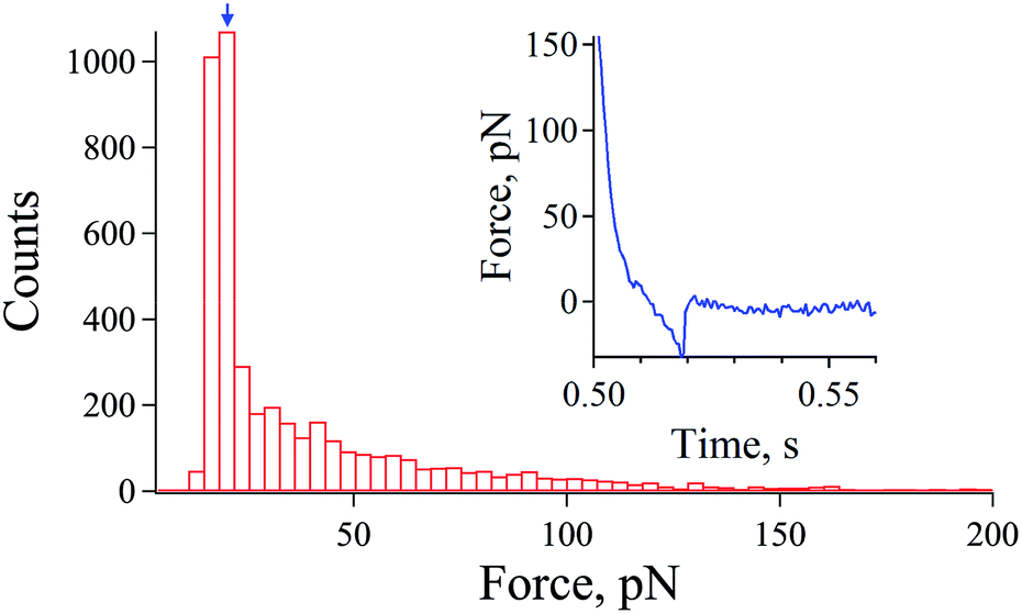 | ||
| Fig. 1 Histogram of observed rupture forces at non-equilibrium unbinding of the streptavidin–biotin system. The inset shows a typical force–distance curve, which contain the rupturing event of the streptavidin–biotin bond. | ||
Results and discussion
Optimization of molecular density on AFM probes and substrates
First, we optimized the density of the system's molecules on the substrate and tip. A histogram of the observed rupture forces (extracted from 22500 force curves) at non-equilibrium unbinding (higher loading rates) was obtained with a Fuzzy logic algorithm developed by Kasas et al.29,30 The histogram of the observed rupture forces evaluated from force curves (inset of Fig. 1) revealed that single molecular pair events are dominant in our AFM measurements.
As shown in Fig. 1, weak rupture forces are dominantly detected given by the modal rupture force (most frequently observed rupture force) of approximately 20 pN (blue arrow), which is in the range of the data observed in a previous study for a streptavidin–biotin single bond.22,31 Although the modal rupture force is low comparing to the results obtained in the pioneering work of Merkel et al., the manner of immobilization of the streptavidin molecules and the buffer system used could actually explain this difference as pointed out by the works of Taninaka et al.22,28,31
This result in Fig. 1 indicates that the chemical functionalization of the tip and substrate employed in this study was optimized for the detection of the single streptavidin–biotin bond.
Monitoring of the interaction force at high temporal resolution
At a slow loading rate of ∼20 pN s−1, a typical force–time curve was obtained as shown in Fig. 2a. In the force–time curve, an adhesion force can be observed as a negative force during retraction due to the bond that is resisting the pulling of the probe.32 When the rupture force is reached, a sudden jump-off can be observed as emphasized by the black rectangle shown in Fig. 2a.26 However, several rebinding and unbinding events after the initial rupture were observed allowing the monitoring of the dynamics of the system in near-equilibrium during the period of biotin recognition by the streptavidin molecule leading to binding, and along the unbinding reaction path in the direction of probe pulling (Fig. 2b).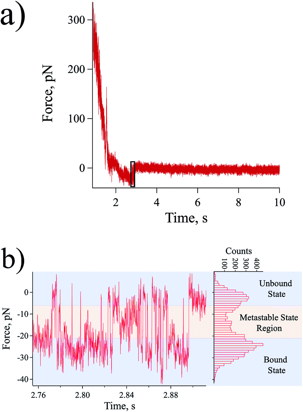 | ||
| Fig. 2 Streptavidin–biotin bond dynamics in near-equilibrium probed at a slow loading rate. (a) Force plotted as a function of time. (b) Magnified force–time plot of black box in (a) and a histogram of force values observed in the force–time plot. Transient events were spotted (green arrows as representatives) suggesting the presence of intermediate metastable states. | ||
At some sufficiently low loading rate, depending on the probe spring constant, the near-equilibrium dynamics of the receptor–ligand system can be explored.13,14 In this quasi-static process, wherein the dynamics of the interaction is considerably faster than the pulling process, the system tends to attain equilibrium allowing the rebinding of the two complementary molecules, thus, the observation of multiple bound-to-unbound and unbound-to-bound state transitions. This also supports to the claim that the detected near-equilibrium forces came from the interaction of a single streptavidin–biotin pair and not from the simultaneously rupturing of multiple streptavidin–biotin bonds. To explain further, due to the stochastic behaviour of proteins,33 one can consider an extremely low probability that multiple bonds always simultaneously unbind and rebind to explain the observed behaviour shown in Fig. 2. Moreover, simultaneous rupturing of multiple bonds would need a rupture force that is way higher than the equilibrium force (force that can allow rebinding process) for a single bond prohibiting any rebinding event to happen.
The histogram in the right of Fig. 2b highlights the population of the states (from initial to final bond rupture) detected in our AFM experiments. The results revealed some distinct intermediate metastable states wherein the system temporarily resides in between its bound and unbound states [metastable state region in Fig. 2b]. A metastable state is considered to be a temporal energy trap or a stable intermediate stage other than the lowest energy well, which may occur at a shorter lifetime.34,35 In our results, each state is expected to be revealed as a force peak in the histogram analyzed as the mean equilibrium force of the combined probe and intermolecular bond system, however, due to their transience, these metastable states are difficult to be resolved individually. Getting a histogram of the whole region of the detected dynamics sums up all the events into an equivocal illustration of the equilibrium forces for the streptavidin–biotin system (Fig. 2b).
Resolving the transient states by segmentation of force–time plots
To resolve the transient states, the force–time curve region in Fig. 2b was divided into several segments starting from the system's initial binding (segment 1) until its final rupture showing the unbound-state-equivalent force distribution (segment 10). Through this, the equivalent force distribution of the probed states can be effectively separated into segments giving more comprehensible histograms with distinct force peaks, which were determined by a multipeak-fitting algorithm.The segments showed different sets of force peaks, thus, the force peaks observed in one segment were carefully compared to the others for a valid interpretation of the data. Some force peaks only showed up in only 1–2 of the 10 segments. These peaks were omitted from interpretation. Other than those, a total of eight force peaks were confirmed and interpreted as the corresponding states of the streptavidin–biotin system. The mean value of these force peaks was calculated and tabulated as shown in Table 1 and represented by the dashed lines in Fig. 3. The reproducibility of the force peaks is described in the ESI.†
| Force peak | 1 | 2 | 3 | 4 | 5 | 6 | 7 | 8 |
| Mean (pN) ± std. dev. | 0 ± 1.04 | −3.20 ± 0.53 | −8.16 ± 0.70 | −14.8 ± 0.8 | −20.5 ± 0.2 | −24.5 ± 0.7 | −29.6 ± 0.7 | −33.0 ± 0.8 |
| Δx (nm) | 4.57 ± 0.14 | 4.13 ± 0.07 | 3.44 ± 0.10 | 2.52 ± 0.12 | 1.73 ± 0.03 | 1.18 ± 0.10 | 0.47 ± 0.10 | 0 ± 0.11 |
| V(Δx) (kcal mol−1) | 0 | −0.10 | −0.66 | −2.19 | −4.19 | −5.99 | −8.73 | −10.9 |
| ΔG0,f (kcal mol−1) | 0 | −1.76 | −1.65 | −0.75 | −0.60 | −1.77 | −1.35 | −1.0 |
| ΔG0 (kcal mol−1) | 0 | −1.86 | −2.31 | −2.94 | −4.79 | −7.76 | −10.08 | −11.9 |
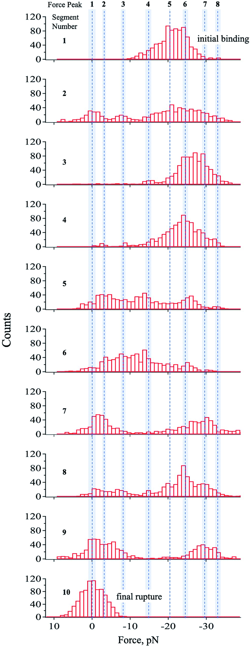 | ||
| Fig. 3 Histograms of each segmented region. The region presented in Fig. 2b was divided into 10 segments, which was optimized by minimizing peak-fitting error. The dashed lines correspond to the mean value of the force peak obtained though multipeak fitting and the shaded region represents the standard deviation. The mean values of force peak 8 and 1 are interpreted as the equivalent force for the lowest bound and unbound states, respectively as suggested by eqn (1). It should be noted that all states were not observed in every segment. A total of 8 states were observed with high reproducibility (ESI†) presented in Table 1 and by the broken lines in this figure. | ||
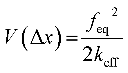
Theoretical background to convert force to potential energy
Next, we attempt to provide an accurate description of the potential landscape for the streptavidin–biotin bond. The Gibbs free energy of a bond is a commonly used parameter to measure the amount of usable energy or the energy that can do work in a system.36,37 The estimation of the Gibbs free energy of the intermolecular interaction in native state can be derived from the energy landscape model of the combined potential of the probe system and the bond.When the intermolecular bond is formed and pulled by a probe, its free energy landscape [G(x)] is distorted by the force probe potential [V(x)] producing another local minimum in the combined potential of the bond and the probe [E(x)] that traps the system's unbound state as depicted in Fig. 4. The original bound state of the system is raised by the probe potential to as much as V(Δx) establishing a new and transient equilibrium condition lowering the bond free energy difference between the bound and unbound states from ΔG0 to ΔG0,f giving the relation,
| ΔG0 = V(Δx)+ ΔG0,f | (1) |
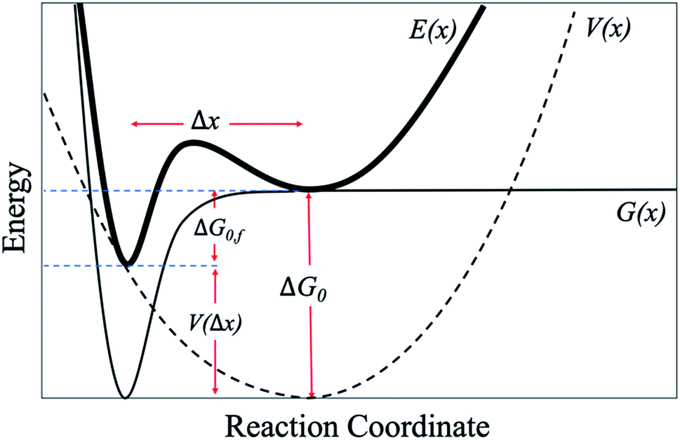 | ||
| Fig. 4 Schematic model of an energy potential landscape for SMFS experiments (ref. 14 and 37). | ||
The first component in eqn (1) is given by,
 | (2) |
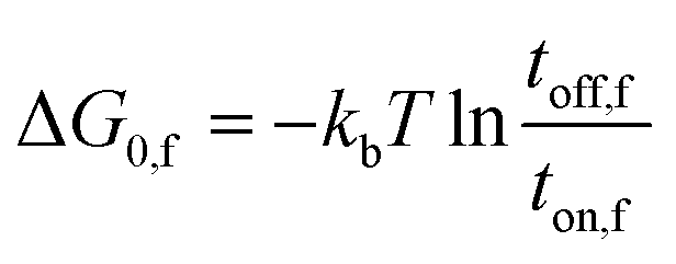 | (3) |
The lifetime of each state was evaluated by a statistical analysis of the force–time plot with a sliding window method [Fig. 5 a and b]. For each window with a size of 10 data points, the standard deviation (std. dev.) value is obtained and plotted against the same time series to reveal the transitions from one state to another as peaks of the std. dev. plot (Fig. 5). By employing a std. dev. threshold obtained by analysing the noise level of the spectroscopic data far from the sample surface, the desired states with their respective corresponding forces were captured and the distance between peaks signifies the state lifetime [Fig. 5b].
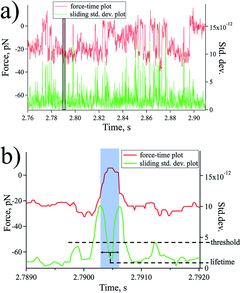 | ||
| Fig. 5 Method to evaluate lifetime of transient states though sliding window method. (a) Force (red, left axis) and std. dev. (green, right axis) plotted against the same time series. (b) Zoomed region (box in (a)) highlighting the peak distance as the lifetime of the state and employing a threshold to capture specific events. | ||
Together with the calculation of ΔG0 using eqn (1), the location of the unbound state relative to the bound state along the reaction coordinate (direction of pulling) can be approximated from the deflection value as expressed below (Fig. 4).38
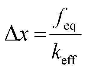 | (4) |
Previous studies concluded that the rupture force in an equilibrium state (extremely slow loading rate) does not depend on the loading rate but on the stiffness of the probe system used.39 Therefore, it is only appropriate to consider the effect of the PEG linker on the effective spring constant of the probe. The effective spring constant was calculated to be 7.2 pN nm−1 using the expression:
 | (5) |
Illustration of potential landscapes
With the series of the histograms representing each segment of the observed streptavidin–biotin dynamics in near-equilibrium, mean force peak values are tabulated (Table 1) together with the corresponding ΔG0 values and relative location through the deflection value Δx, as calculated using eqn (1) and (4), respectively.Some prominent force peaks were observed – force peak 4, 5, 6, 7, and 8 – as suggested by their high ΔG0 magnitude values and their corresponding standard deviations that are two orders in magnitude lower than the mean value. Force peak 8 with a mean value of −33.0 pN is considered to be representing the lowest energy bound state (designated, for simplicity, as position 0) for the streptavidin–biotin system since this corresponds to the largest |ΔG0| of 11.9 kcal mol−1. This value widely differs from results obtained in bulk ensemble measurements (|ΔG0| ≈ 20 kcal mol−1),40–42 which can be expected. However, as compared to other single-molecule experiments, this still seems to be an underestimation on the binding free energy of the system.1,2 One possible reason is that our measurements, for practical reasons, probes the system in near-equilibrium under the quasi-static assumption as discussed earlier. Notably, in a recent paper by Rico et al. where they explored the streptavidin–biotin free energy landscape through combining molecular dynamics and high-speed force spectroscopy, they reported the system's lowest binding free energy to be ∼12 kcal mol−1 (21kbT) – a value that is close to what we have obtained.43 In this case, it is clear that further studies still have to be performed to reason the discrepancy of the calculated binding energy.
The remaining prominent force peaks (4, 5, 6, and 7) are considered to be the mean equilibrium forces for the prominent intermediate metastable states of the streptavidin–biotin system. Force peaks 6 and 7 expressed a corresponding ΔG0 value of −7.76 and −10.08 kcal mol−1, respectively. These intermediate metastable states, which are positioned at 1.18 and 0.473 nm, respectively from the lowest energy bound state, are also revealed and indicated by the results of previous studies.1,2 In the paper of Pincet and Husson, a reinterpretation of the data from the molecular dynamics simulation of Izrailev et al. and the data from BFP experiments of Merkel et al. confirmed that two prominent intermediate metastable states are present in the streptavidin–biotin system located approximately at 1.09 and 0.39 nm from the bound state. This is in good agreement with the calculated locations obtained from the near-equilibrium force microscopy performed in our study.
In the paper of Merkel et al., an additional intermediate metastable state, other than the two already mentioned, was revealed through dynamic force spectroscopy. Moreover, in the investigation of the system through molecular mechanics calculation of rupture force, the simulations suggest a multiple-pathway rupture mechanism involving five major unbinding steps attributed to hydrogen bond interactions of the biotin ligand and the streptavidin binding site residues.23 This is also in accordance with the results presented by Livnah et al. and Weber et al. where they implicitly demonstrated through the structural investigation of the three-dimensional crystallographic images of streptavidin–biotin complex that no less than five protein residues form a hydrogen bond with the biotin ureido group (in addition to van der Waals interactions present between biotin and streptavidin). These results clearly give a basis to the findings displayed in Table 1. In addition to the previously mentioned force peaks 6 and 7, two more prominent force peaks: 4 (ΔG0 = −2.94 kcal mol; Δx = 2.52 nm) and 5 (ΔG0 = −4.79 kcal mol; Δx = 1.73 nm) were revealed corresponding to two more intermediate metastable states that can be attributed to a strong binding such as a hydrogen-bond interaction.44
Two more metastable states are revealed in force peak 3 (ΔG0 = −2.31 kcal mol; Δx = 3.44 nm) and force peak 2 (ΔG0 = −1.86 kcal mol; Δx = 4.13 nm). Their corresponding locations from the lowest bound state would suggest that these weak interactions occur beyond the binding pocket of streptavidin as the PEG-attached biotin molecule is on its way out of streptavidin. This is a finding that was also observed in the paper of Merkel et al. where they speculated that some flexible protein structures or non-specific interaction occurring at the outer surface of streptavidin can be the origin of the interaction.
Furthermore, the overall distance range observed in this study is in good agreement to the experimentally determined size of the streptavidin–biotin system, which shows to be around 133 nm3.45 Assuming a spherical shape, this would give a diameter of 6.33 nm.
This information of the states' free energy values and their corresponding location can be complemented with the location of energy barriers obtained through DFS and computer simulations to give a whole unambiguous picture of the streptavidin–biotin energy potential landscape (Fig. 6).1,2 In summary, a total of six intermediate metastable states were revealed in this study, four of which are attributed to the strong hydrogen bond interactions between the residues at the streptavidin binding site and biotin. Two of those are prominent metastable states with high free energy values, which are also revealed in previous studies of the system. The last two suggested intermediate metastable state exhibiting a low free energy value and are located far away from the lowest bound state can be attributed to van der Waals interaction between the ligand and the flexible elements of the protein beyond the binding site or to any nonspecific interactions experienced by the system that allowed the detection of weak metastable states along its energy landscape.46
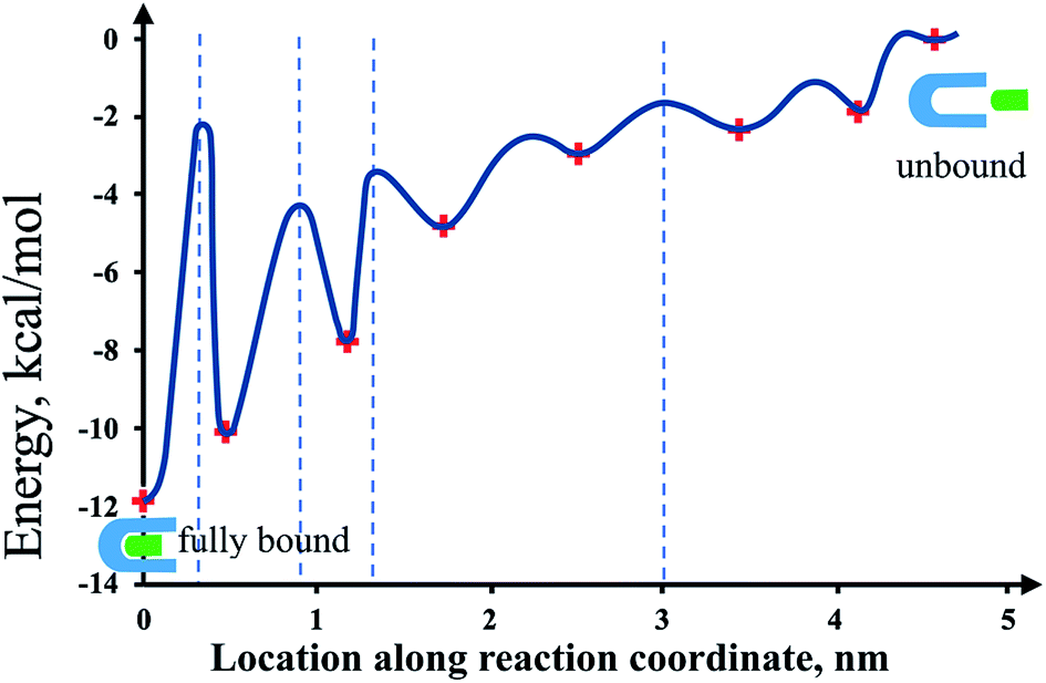 | ||
| Fig. 6 Illustration of energy potential landscape using the results obtained in this study. This shows the location of the various states (lowest bound, metastable, and unbound) with the corresponding bond free energy (+markers). The blue dashed lines represent the locations of the energy barriers revealed in previous studies.1–3 The presence of the other energy barriers is implied by the adjacent energy minima. Note: the curvature of the energy states and the barrier locations other than the already reported values are arbitrary just to show a simplified illustration of the potential landscape. | ||
Conclusions
In this work, we succeeded in the illustration of the whole energy potential landscape of the streptavidin–biotin bond. Our key technique was the observation of the dynamics of the system in high temporal resolution by AFM. The technique enabled the detection of the locations of the metastable states relative to the lowest bound state along with minimal distortion of the system's energy landscape This is a great leap towards uncovering the binding mechanism of the ligand molecule, biotin to its receptor, streptavidin. Various previous studies only revealed the locations of some energy barriers implying the presence of adjacent metastable states and/or generate an energy landscape from non-equilibrium unbinding experiments which has a greater possibility of bypassing transient states. Our study complemented the previous studies by the determination of the relative positions of the intermediate metastable states along the reaction coordinate.Several studies have been focusing on the investigation of the streptavidin–biotin system showing discrepancies in results. The findings presented in our study bridge the gaps, showing that the results of several experimental and simulation works are pieces of information from the overall sophisticated nature of this receptor–ligand system. In the paper of Pincet and Husson, it was suggested that the history of the bond might be the origin of the streptavidin–biotin paradox. This goes in parallel with our findings and could be a consequence of the stochastic behaviour of the system, that is, several intermediate metastable states are present where the system can possibly reside during the recognition process of streptavidin and biotin enhancing the stability of the bond. Although an energy landscape can give a substantial information on the mechanism and nature of binding, having a vivid picture on the conformational states in parallel with the energy landscape is something that still needs to be done for a full understanding of the system. Finally, we expect that this extraction of information in a molecular level can pave the way to a more advanced kind of research, such as the discovery of novel drugs and proteins for biomedical applications.
Conflicts of interest
There are no conflicts to declare.Acknowledgements
The author (T. H.) acknowledges the financial supports by KAKENHI (19H02565, 17K20095 and 15KK0184) and JST-PRESTO. The authors appreciate the help of Ms Kazue Taki for the administration of this project.Notes and references
- R. Merkel, P. Nassoy, A. Leung, K. Ritchie and E. Evans, Nature, 1999, 397, 50–53 CrossRef CAS PubMed.
- F. Pincet and J. Husson, Biophys. J., 2005, 89, 4374–4381 CrossRef CAS PubMed.
- S. Izrailev, S. Stepaniants, M. Balsera, Y. Oono and K. Schulten, Biophys. J., 1997, 72, 1568–1581 CrossRef CAS PubMed.
- E. P. Diamandis and T. K. Christopoulos, Clin. Chem., 1991, 37, 625–636 CAS.
- O. Livnah, E. A. Bayer, M. Wilchek and J. L. Sussman, Proc. Natl. Acad. Sci. U. S. A., 1993, 90, 5076–5080 CrossRef CAS PubMed.
- P. C. Weber, D. H. Ohlendorf, J. J. Wendoloski and F. R. Salemme, Science, 1989, 243, 85–88 CrossRef CAS PubMed.
- Avidin-Biotin Technical Handbook, Thermo Fischer Scientific, Inc., US, 2009 Search PubMed.
- N. Bocquet, J. Kohler, M. N. Hug, E. A. Kusznir, A. C. Rufer, R. J. Dawson, M. Hennig, A. Ruf, W. Huber and S. Huber, Biochim. Biophys. Acta, 2015, 1848, 1224–1233 CrossRef CAS PubMed.
- M. Seifert, M. T. Rinke and H. J. Galla, Langmuir, 2010, 26, 6386–6393 CrossRef CAS PubMed.
- P. D. Ashby, in Handbook of Molecular Force Spectroscopy, Springer, 2008, pp. 273–285 Search PubMed.
- E. Evans, Faraday Discuss., 1998, 111, 1–16 RSC.
- E. Evans, Annu. Rev. Biophys. Biomol. Struct., 2001, 30, 105–128 CrossRef CAS PubMed.
- R. W. Friddle, P. Podsiadlo, A. B. Artyukhin and A. Noy, J. Phys. Chem. C, 2008, 112, 4986–4990 CrossRef CAS.
- A. Noy, Curr. Opin. Chem. Biol., 2011, 15, 710–718 CrossRef CAS PubMed.
- A. Noy, Handbook of molecular force spectroscopy, Springer Science & Business Media, 2007 Search PubMed.
- Y. Arai, K. Okabe, H. Sekiguchi, T. Hayashi and M. Hara, Langmuir, 2011, 27, 2478–2483 CrossRef CAS PubMed.
- S. O. Kim, J. A. Jackman, M. Mochizuki, B. K. Yoon, T. Hayashi and N. J. Cho, Phys. Chem. Chem. Phys., 2016, 18, 14454–14459 RSC.
- M. Mochizuki, M. Oguchi, S. O. Kim, J. A. Jackman, T. Ogawa, G. Lkhamsuren, N. J. Cho and T. Hayashi, Langmuir, 2015, 31, 8006–8012 CrossRef CAS PubMed.
- C. Yuan, A. Chen, P. Kolb and V. T. Moy, Biochemistry, 2000, 39, 10219–10223 CrossRef CAS PubMed.
- J. Wong, A. Chilkoti and V. T. Moy, Biomol. Eng., 1999, 16, 45–55 CrossRef CAS PubMed.
- I. J. General, R. Dragomirova and H. Meirovitch, J. Phys. Chem. B, 2012, 116, 6628–6636 CrossRef CAS PubMed.
- A. Taninaka, O. Takeuchi and H. Shigekawa, Int. J. Mol. Sci., 2010, 11, 2134–2151 CrossRef CAS PubMed.
- H. Grubmuller, B. Heymann and P. Tavan, Science, 1996, 271, 997–999 CrossRef CAS PubMed.
- M. J. Fischer, Methods Mol. Biol., 2010, 627, 55–73 CrossRef CAS PubMed.
- C. K. Riener, C. M. Stroh, A. Ebner, C. Klampfl, A. A. Gall, C. Romanin, Y. L. Lyubchenko, P. Hinterdorfer and H. J. Gruber, Anal. Chim. Acta, 2003, 479, 59–75 CrossRef CAS.
- H. J. Butt, B. Cappella and M. Kappl, Surf. Sci. Rep., 2005, 59, 1–152 CrossRef CAS.
- J. L. Hutter and J. Bechhoefer, Rev. Sci. Instrum., 1993, 64, 3342 CrossRef CAS.
- A. Taninaka, Y. Hirano, O. Takeuchi and H. Shigekawa, Int. J. Mol. Sci., 2012, 13, 453–465 CrossRef CAS PubMed.
- S. Kasas, B. M. Riederer, S. Catsicas, B. Cappella and G. Dietler, Rev. Sci. Instrum., 2000, 71, 2082–2086 CrossRef CAS.
- H. Tahara, T. Nyu, E. A. Q. Mondarte, T. Maekawa and T. Hayashi, Adv. Mater. Phys. Chem., 2018, 217–226 CrossRef.
- A. Taninaka, O. Takeuchi and H. Shigekawa, Phys. Chem. Chem. Phys., 2010, 12, 12578–12583 RSC.
- B. Voigtländer, Scanning Probe Microscopy, Springer, 2016 Search PubMed.
- A. Fersht, Structure and mechanism in protein science: a guide to enzyme catalysis and protein folding, World Scientific, 2017 Search PubMed.
- The Editors of Encyclopaedia Britannica, Metastable State, Encyclopedia Britannica, Inc, 1998 Search PubMed.
- A. R. Dinner and M. Karplus, Nat. Struct. Biol., 1998, 5, 236–241 CrossRef CAS PubMed.
- J. Donald, J. Voet and W. Charlotte Pratt, Principles of Biochemistry, John-Wiley Inc., New York, 2008 Search PubMed.
- R. Glaser, Biophysics: an introduction, Springer, Heidelberg, 2012 Search PubMed.
- A. Noy, Scanning, 2008, 30, 96–105 CrossRef CAS PubMed.
- A. Noy and R. W. Friddle, Methods, 2013, 60, 142–150 CrossRef CAS PubMed.
- N. M. Green, Methods Enzymol., 1990, 184, 51–67 CAS.
- M. Wilchek and E. A. Bayer, Methods Enzymol., 1990, 184, 5–13 CAS.
- D. E. Hyre, I. Le Trong, E. A. Merritt, J. F. Eccleston, N. M. Green, R. E. Stenkamp and P. S. Stayton, Protein Sci., 2006, 15, 459–467 CrossRef CAS PubMed.
- F. Rico, A. Russek, L. González, H. Grubmüller and S. Scheuring, arXiv, 2018.
- S. Y. Sheu, D. Y. Yang, H. L. Selzle and E. W. Schlag, Proc. Natl. Acad. Sci. U. S. A., 2003, 100, 12683–12687 CrossRef CAS PubMed.
- C. S. Neish, I. L. Martin, R. M. Henderson and J. M. Edwardson, Br. J. Pharmacol., 2002, 135, 1943–1950 CrossRef CAS PubMed.
- Using two other force curves in the data set, an analogous scatter diagram of the intermediate metastable states of the system's energy potential landscape was generated. This supports the locations of each state along the reaction coordinate of bond pulling (see Fig. 1s in ESI†). Moreover, a collection of all detected states from the data set of segmented force curves were also summarized in the ESI (Fig. 2s).†.
Footnote |
| † Electronic supplementary information (ESI) available. See DOI: 10.1039/c9ra04106k |
| This journal is © The Royal Society of Chemistry 2019 |