Controlling magnetic coupling in bi-magnetic nanocomposites

Abstract

Magnetic nanocomposites constitute a vital class of technologically relevant materials, in particular for next-generation applications ranging from biomedicine, catalysis, and energy devices. Key to designing such materials is determining and controlling the extent of magnetic coupling in them. In this work, we show how the magnetic coupling in bi-magnetic nanocomposites can be controlled by the growth technique. Using four different synthesis strategies to prepare prototypical LaFeO₃–CoFe₂O₄ and LaFeO₃–Co_0.5Zn_0.5Fe₂O₄ nanocomposite systems, and by performing comprehensive magnetic measurements, we demonstrate that the final material exhibits striking differences in their magnetic coupling that is distinct to the growth method. Through structural and morphological studies, we confirm the link between the magnetic coupling and growth methods due to distinct levels of particle agglomeration at the very microscopic scale. Our studies reveal an inverse relationship between the strength of magnetic coupling and the degree of particle agglomeration in the nanocomposites. Our work presents a basic concept of controlling the particle agglomeration to tune magnetic coupling, relevant for designing advanced bi-magnetic nanocomposites for novel applications.

---

1. Introduction

Bi-magnetic nanocomposites and low-dimensional materials (e.g., core–shell systems) are of huge scientific and technological interest, and can be used in a variety of applications, such as in biomedicine and catalysis,^1–9 for electromagnetic functions such as electromagnetic wave absorption and shielding,^10–12 and improving functional properties such as obtaining room temperature giant magnetoresistance.¹³ The wide range of possible applications has triggered intense research activities in the field in recent years. Particularly interesting are magnetic nanocomposites consisting of strongly correlated electron oxides as the individual components. The cross-correlated electronic and magnetic properties of such complex oxides offer ample opportunities for scientists to probe into a variety of exciting and intriguing phenomena occurring in these systems.¹⁴ In addition to the already diverse spectrum of properties, reducing the particle size to the nanoscale regime results in several new properties vis-á-vis the bulk compounds,^15–20 and provides a new dimension to explore. The complexity is further increased when one looks at nanocomposites of strongly correlated electron oxide systems.^21,22 In such a scenario, it is extremely important to be able to control and determine the magnetic coupling in such materials, so as to design materials that are custom-made for specific applications, for example, for creating magnetoelectric devices where the interfacial exchange coupling between a multiferroic material and a ferromagnet can be used to switch the magnetization of the ferromagnetic layer.²³

In this paper, we discuss the effect of synthesis technique on the extent of magnetic coupling and thus on the magnetic properties of bi-magnetic nanocomposites of strongly correlated electron oxide systems. To demonstrate our findings, we have chosen LaFeO₃–CoFe₂O₄ (LFO–CFO) and LaFeO₃–Co_0.5Zn_0.5Fe₂O₄ (LFO–CZFO) as prototypical nanocomposite systems. The two individual phases, LFO and CFO, represent perfect models for two classes of materials with remarkable physical properties. LFO is a canted G-type antiferromagnet with a high ordering temperature of ∼750 K.²⁴ It has an orthorhombic perovskite structure, in which the Fe³⁺ ion is surrounded by six O²⁻ ions and forms an octahedron. The Fe³⁺ spins are coupled antiferromagnetically with opposite spin direction between two sub-lattices. When the particle size is reduced, spin canting of Fe ions increases at the surface of the particle, and hence, decreasing the particle size is expected to tune the magnetic properties of LFO.^25–27 Recently, LFO has also been reported to be multiferroic with ferroelectric hysteresis loops observed at room temperature.²⁸ Thin films of LFO are excellent model systems for exploring the correlation between their structure and antiferromagnetic domains, and the resulting physical mechanisms that occur when it is coupled to a ferromagnetic layer.²⁹ In contrast, the magnetic properties of LFO nanopowders coupled to a ferromagnetic system have been relatively less studied. The second phase in the nanocomposites, CFO, is a typical ferrimagnet (ordering temperature ∼800 K) exhibiting high saturation magnetization, high coercivity, and large magnetic anisotropy that can be tuned by doping.³⁰ Studies that combine multiferroic LFO with a ferrimagnetic spinel system are relatively rare, although this combination is a promising candidate for improving the magnetic properties of LFO that can then be used in applications such as sensors, data storage media, spintronic devices, and multiple stage memories.^23,31 Some studies have indicated that the magnetic interaction between the LFO and CFO phases in LFO–CFO nanocomposites is antiferromagnetic in nature.³² Such studies have focused exclusively on physically-mixed samples, where the two phases were mechanically ground in appropriate proportions to form composite systems.^32,33 In the current study, our main motivation was to use different synthesis techniques, primarily chemical synthesis routes, and throw light on the effect of synthesis technique on the strength of magnetic coupling between the LFO and CFO phases. The two individual components, LFO and CFO, can be synthetized with controlled structural and morphological properties using relatively easy synthesis routes. In addition, the flexible crystal chemistry of the spinel structure of CFO opens up the possibility of designing different nanocomposites with tunable magnetic properties. As an example, Zn-doped CFO, Co_0.5Zn_0.5Fe₂O₄ (CZFO), was chosen to demonstrate the effect of magnetic anisotropy (details in later sections). We will show that the followed synthesis routes have a profound effect on the magnetic coupling of the resultant nanocomposite. Equally importantly, the effect is not always obvious from routine magnetization measurements, and requires more detailed and in-depth studies. In the following sections, we will first present the synthesis strategies used to prepare the different nanocomposite samples, followed by the magnetic characterization, and analysis of the data.

2. Synthesis and experimental techniques

2.1. Synthesis

In this section, we describe the synthesis strategies followed to prepare five different samples, labeled S1, S2, S3, S3′, and S4.

S1: S1 is an LFO–CFO nanocomposite prepared by physically mixing the two individual components (LFO and CFO). The individual components were chemically synthesized via sol–gel self-combustion synthesis technique. The details of the synthesis of the individual components can be found in our earlier publications.^22,34,35 The individual LFO and CFO particles have a crystallite size of ∼20 nm. High-resolution transmission electron microscopy (TEM) images showing individual grains of LFO and CFO can be found in our earlier publication.²² S1 was then prepared by physically mixing the LFO and CFO nanoparticles (weight fraction LFO : CFO = 98 : 02) in a mortar with acetone to obtain a fine mixture of the two powders.

S2: S2 was prepared by first dispersing an appropriate amount of the pre-synthesized 20 nm CFO nanoparticles (final weight fraction of CFO in the nanocomposite = 2%) in deionized water and sonicating it for ∼30 min. Stoichiometric amounts of the precursors of LFO i.e., La(NO₃)₃·6H₂O and Fe(NO₃)₃·9H₂O (Sigma-Aldrich), were then added and dissolved at room temperature. To this solution, ethylene glycol was added to act as the chelating agent. The clear solution was then heated to 80 °C and stirred for 20 min. Next, the temperature was increased and maintained at ∼150 °C till the formation of a gel. The temperature was then increased to ∼250 °C when a self-combustion reaction with flame occurred, yielding a fluffy powder. The powder was crushed in a mortar, transferred to a furnace, and annealed in air at 350 °C for 1 h, followed by a further annealing at 450 °C for an additional 1 h, and finally at 500 °C for 10 h.

S3 and S3′: S3 was prepared using the exact same steps as S2, except that the pre-synthesized CFO nanoparticles used in this case were prepared using a different technique as compared to the 20 nm CFO nanoparticles that were used for S2. For S3, the CFO nanoparticles used were prepared using a solvothermal method in an autoclave, resulting in CFO nanoparticles that were smaller in size (∼5 nm), and more well-dispersed compared to the more aggregated CFO nanoparticles used for preparing S2. The synthesis procedure has been described in detail elsewhere³⁶ and here just a brief description is given. First, a water/1-pentanol solution of NaOH was prepared and after that an adequate volume of oleic acid, which served as capping agent for preventing nanoparticle aggregation, was added with stirring. Cobalt(II) nitrate hexahydrate, iron(III) nitrate nonahydrate, and zinc(II) nitrate hexahydrate (for CZFO) were mixed in stoichiometric quantities and dissolved in distilled water. This mixture was poured into the above solution and kept under vigorous stirring for 1 h. The synthesis was performed at 180 °C for 8 h. The two samples were then dispersed in water using a mild exchange ligand process.

An appropriate amount of the 5 nm CFO nanoparticles (in suspension) was then added to deionized water, and the exact same steps as described for S2 were followed to obtain the S3 nanocomposite. S3′ was prepared using the exact same steps as S3, except that instead of using 5 nm, well-dispersed CFO nanoparticles, we used 5 nm, well-dispersed Co_0.5Zn_0.5Fe₂O₄ nanoparticles to prepare LFO–CZFO nanocomposites.

S4: S4 was prepared using a modified sol–gel technique. Instead of using pre-formed CFO nanoparticles, two sols (one containing stoichiometric amounts of the precursors of CFO i.e., Co(NO₃)₂·6H₂O and Fe(NO₃)₃·9H₂O (Sigma-Aldrich), and the other containing stoichiometric amounts of the precursors of LFO i.e., La(NO₃)₃·6H₂O and Fe(NO₃)₃·9H₂O (Sigma-Aldrich)) were prepared separately at room temperature. The two clear solutions were then mixed at room temperature and stirred for 20 min. This composite sol was then heated to 80 °C and stirred for 20 min. Next, the temperature was increased and maintained at ∼150 °C till the formation of a gel. The temperature was then increased to ∼250 °C when a self-combustion reaction with flame occurred, yielding a fluffy powder. The powder was crushed in a mortar, transferred to a furnace, and annealed in air at 350 °C for 1 h, followed by a further annealing at 450 °C for an additional 1 h, and finally at 500 °C for 10 h.

The samples that are investigated in this study are summarized in Table 1.

Table 1 List of nanocomposites

Sample name	Composition	Synthesis method
S1	LaFeO3–CoFe2O4	Physical mixing the individual components
S2	LaFeO3–CoFe2O4	Chemical synthesis of LaFeO3 around pre-formed 20 nm, relatively aggregated CoFe2O4 nanoparticles
S3	LaFeO3–CoFe2O4	Chemical synthesis of LaFeO3 around pre-formed 5 nm, well-dispersed CoFe2O4 nanoparticles
S3′	LaFeO3–Co0.5Zn0.5Fe2O4	Chemical synthesis of LaFeO3 around pre-formed 5 nm, well-dispersed Co0.5Zn0.5Fe2O4 nanoparticles
S4	LaFeO3–CoFe2O4	Chemical synthesis of LaFeO3 and CoFe2O4 using a composite sol

---

2.2. Characterization techniques

The samples were characterized by X-ray powder diffraction (XRPD) obtained using a D-5000 diffractometer with CuK_α radiation operating at 40 kV and 30 mA. The data were collected in the range 2θ = 20–70°, with a step size of 0.02°. The XRPD patterns were also used to estimate the average crystallite size of the samples, using the Williamson Hall plot.³⁷

Inductively coupled plasma optical emission spectroscopy (ICP–OES) was carried out for elemental analysis with an iCAP 6300 DUP ICP–OES spectrometer (ThermoScientific). The samples were digested in aqua regia (HCL 37% v/v–HNO₃ 69% v/v 3 : 1) for 8 h, then diluted using Milli-Q water, and analyzed.

Differential thermal analysis (DTA)/thermogravimetric analysis (TGA) were performed using a LabsysEvo 1600 DTA/TGA (Setaram). 10 mg of sample obtained after self-combustion was put in an alumina crucible and heated from 30 to 1000 °C, at 10 °C min⁻¹ under an O₂ atmosphere (20 ml min⁻¹). The DTA and TGA curves were elaborated using the dedicated software Calisto (Setaram).

TEM analysis was performed using a Philips CM200 microscope operating at 200 kV and equipped with a LaB₆ filament. For TEM observations, the samples, in the form of powder, were prepared using the following procedure. A small quantity of powder was dispersed in isopropyl alcohol and subjected to ultrasonic agitation for approximately one minute. A drop of suspension was deposited on a commercial TEM grid covered with a thin carbon film; finally, the grid was kept in air until complete evaporation of the isopropyl alcohol.

Magnetic field-dependent magnetization of the samples was collected using a superconducting quantum interference device (SQUID) magnetometer from Quantum Design Inc. Magnetic hysteresis loops were recorded at T = 5 K in the −5 T to +5 T field range.

3. Results and discussion

3.1. Structural and morphological characterization

The XRPD patterns of the synthesized samples are shown in Fig. 1. The observed reflections can be indexed to the orthorhombic structure of LFO (s.g. Pnma), and no impurity or secondary phase was observed. The CFO (and CZFO) phases remain undetected because of their extremely low fraction in the nanocomposites (only ∼2% by weight). The average crystallite size (D_XRPD) of the samples was calculated from the XRPD data using the Williamson Hall plot,³⁷ and was found to be ∼20 nm.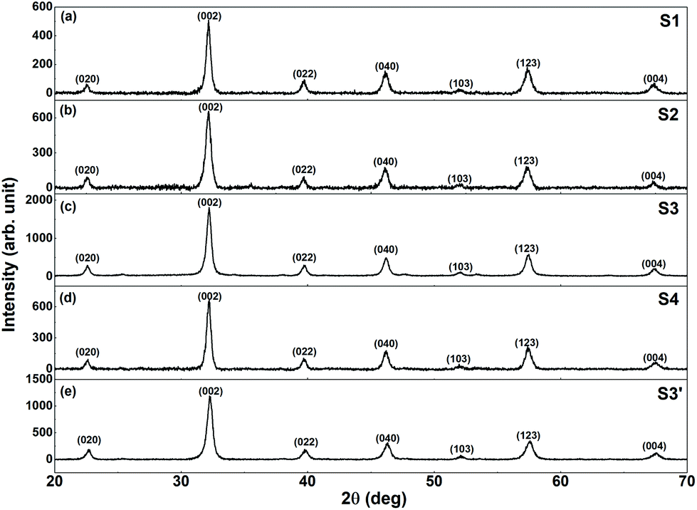

Fig. 1 XRPD patterns of (a) S1, (b) S2, (c) S3, (d) S4, and (e) S3′.

ICP analyses were performed to determine the exact LaFeO₃–CoFe₂O₄ (Co_0.5Zn_0.5Fe₂O₄ for S3′) ratios in the final composites, and were found to be 97.5 : 2.5, 96.7 : 3.3, 99.1 : 0.9, 98.9 : 1.1, and 97.7 : 2.3 for S1, S2, S3, S3′, and S4, respectively. All the values were affected by a systematic error of approximately 5%. Moreover, in S3′ the Co/Zn ratio was equal to 1 : 1 confirming the nominal stoichiometry.

All the samples, were analysed by means of DTA/TG, except S1 (i.e., the sample prepared by physical mixing of the individual components) that is just a reference sample for magnetization measurements. The DTA/TG curves are shown in the ESI (Fig. S1†). It is interesting to observe that above ∼200 °C (∼150 °C for S4), there is a considerable variation in the TG curves consistent with previous reported data.²² In particular, all the samples presented a first loss up to 500 °C, temperature at which a second effect started up to ∼650 °C. The simultaneous DTA analyses reveals the presence of an exothermic peak (at T ≈ 320 °C, 340 °C, and 190 °C for S3, S3′, and S4, respectively) corresponding to the TG variations suggesting the combustion of the unburned organic reagents occurred. It is worth noting that for all the samples, the last step in the TG curves starts at approximately 500 °C, demonstrating that the annealing temperature chosen is enough for removing the organic precursors completely. Overall, the weight lost was approximately 30% for S2, S3, S3′, and approximately 20% for S4. Although the detailed investigation of the synthesis mechanism is beyond the scope of this paper, DTA/TG analysis clearly suggests that the magnetic phase formation in S4 shows a different thermal history that deserves special attention, and a more careful investigation is planned for the near future.

The morphology of the samples S1, S2, and S3 as observed from TEM imaging have been reported in our earlier publications.^21,22 Considering that, a schematic representation showing the level of aggregation of the individual components is illustrated in Fig. 2. The different synthesis strategies are also briefly mentioned in Fig. 2. To prepare S1, the two phases (LFO and CFO) were mixed in the solid state i.e., the individual powders were mixed by mechanically grinding in a mortar to form a physical mixture. This results in a sample that has large aggregates of the two phases, denoted by the large blue and green clusters in Fig. 2a. S2 was prepared by first sonicating the CFO particles in water for several minutes, and then growing the LFO phase in solution. The sonication served to break up the CFO particles into smaller clusters (compared to S1). This is represented by the smaller blue clusters in Fig. 2b. In particular, previous studies reported in our earlier publications^21,22 have shown that the number of CFO particles forming a single aggregate is of the order of thousands of particles in physically-mixed samples like S1, while in S2, the CFO aggregates are composed of few tens of particles at the maximum. The CFO particles used for preparing S3 were synthesized using a solvothermal method that resulted in smaller size CFO particles that are stable in aqueous suspension. Thus, the CFO phase in S3 was even less aggregated compared to S2, as denoted by the small individual blue spheres in Fig. 2c. To prepare S4, we did not use pre-synthesized CFO particles. In contrast, both the CFO and LFO phases were prepared in solution at the same time. This ensured that the CFO particles did not get the opportunity to form clusters, but were formed within the LFO matrix, as denoted schematically in Fig. 2d. We note here that Fig. 2 gives a schematic and qualitative representation of the degree of agglomeration in the samples prepared using the four different techniques. Further studies involving theoretical modeling of the magnetic behavior with the degree of agglomeration as a control parameter might provide a more quantitative description of the aggregation level. This is, however, out of the scope of the present paper.

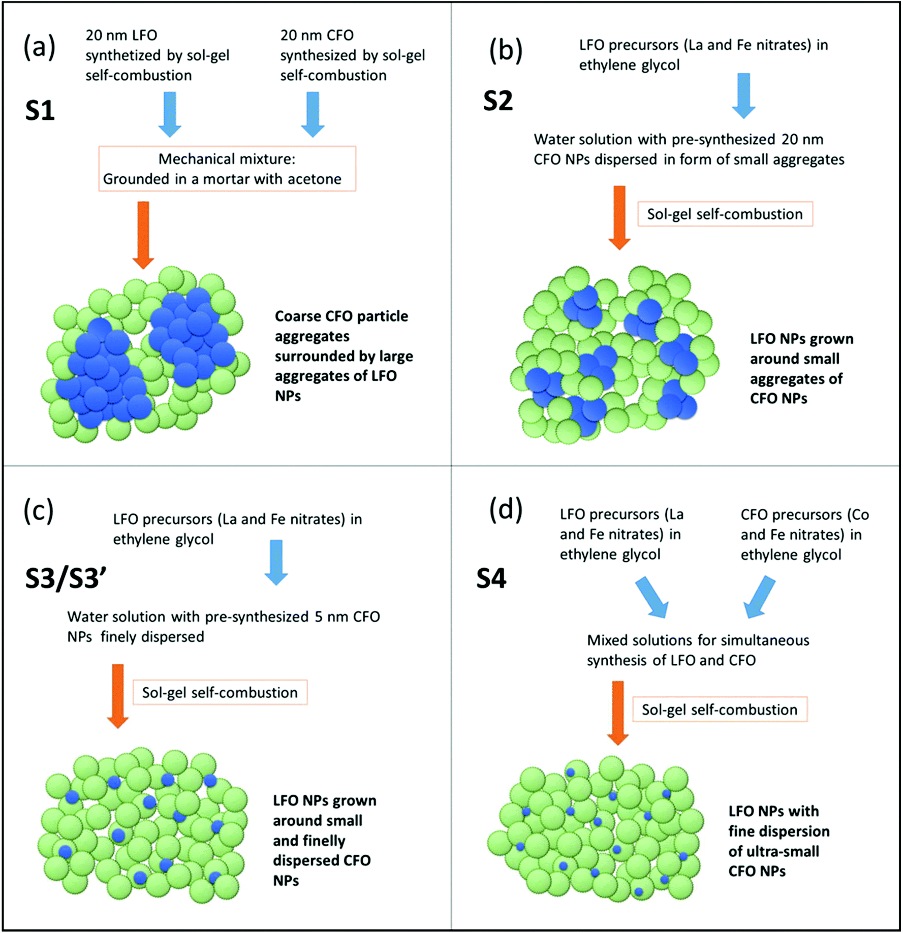Fig. 2 Schematic representation of the different synthesis strategies used that yield samples with different levels of agglomeration. Green and blue spheres indicate LFO and CFO (or CZFO), respectively.

Next, we discuss the morphology of sample S4 that was prepared using a new synthesis route not reported previously. In Fig. 3a, a typical TEM bright field image of sample S4 is shown. The sample is composed of agglomerates of highly interconnected nanocrystals. Some pores are indicated by arrows in Fig. 3a. Selected area electron diffraction (SAED) measurements performed on numerous agglomerates have revealed the crystalline nature of the sample. A typical SAED pattern is shown in Fig. 3b. The diffraction intensity is distributed on rings, revealing the polycrystalline nature of the sample and the random orientation of the crystals. All the diffraction rings can be attributed to the LFO phase and it is difficult to evidence the presence of CFO crystals due to their low fraction (≈2 wt%) in the nanocomposites. The white arrows indicate two very feeble diffraction spots that can be attributed to the {131}_CFO lattice planes.

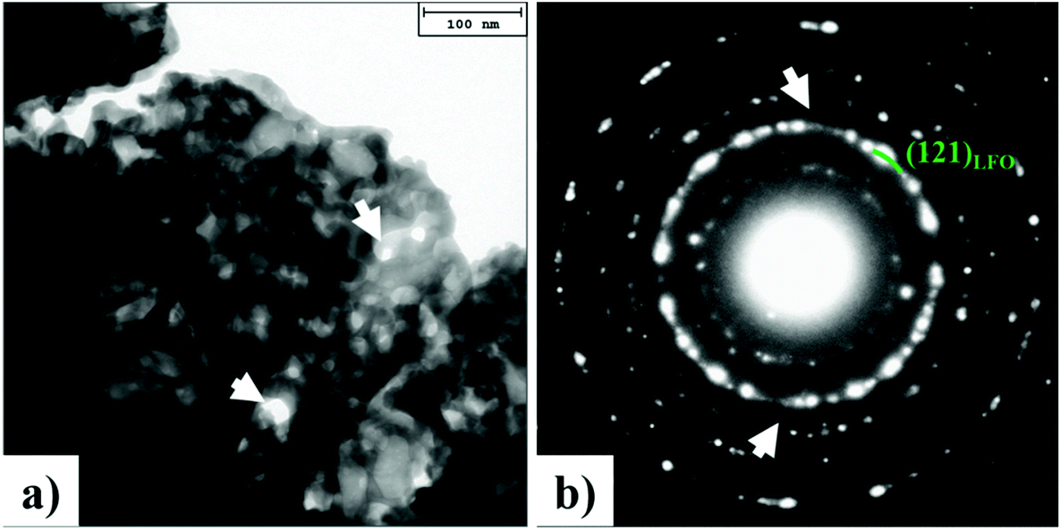Fig. 3 Sample S4: (a) TEM bright field image and (b) corresponding selected area electron diffraction pattern. The arrows in (a) indicate some pores present in the nanocomposite. The positions of very feeble diffraction spots attributable to the CFO phase are indicated by white arrows in (b).

To facilitate the TEM analysis of the CFO phase in the nanocomposite, and to obtain information about the existence and good dispersion of the embedded magnetic phase, another sample was synthesized by the same procedure used for S4 but with a different CFO/LFO ratio. The sample S4′ contained 25% CFO in weight. A typical bright field TEM image of S4′ is reported in Fig. 4a.

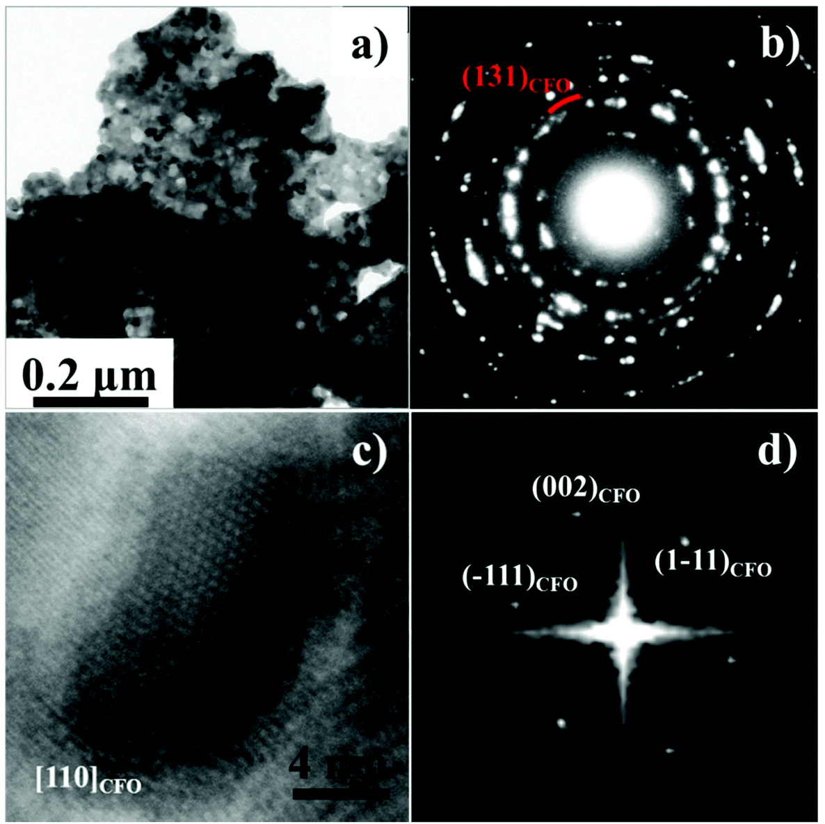Fig. 4 Sample S4′: (a) TEM bright field image, (b) corresponding selected area electron diffraction pattern, (c) high resolution TEM (HRTEM) image of a CFO nanocrystal, and (d) corresponding fast Fourier transform of the image revealing that the CFO crystal is in [110] zone axis.

An agglomerate made of highly interconnected nanocrystals and pores is clearly visible. The corresponding SAED pattern is shown in Fig. 4b. All the diffraction rings can be attributed to the LFO phase except one that can be assigned to the {131}_CFO lattice planes. The uniform and feeble intensity distribution of this ring suggests a small dimension of the CFO crystals. One of the larger CFO nanocrystals is shown in the high-resolution TEM image of Fig. 4c, but smaller crystals are also present (ESI, Fig. S2†). The fast Fourier transform of the image reveals that the CFO crystal is in [110] zone axis, Fig. 4d.

The small dimension of the CFO nanocrystals and their homogenous distribution were further investigated by TEM dark field measurements performed both on small and large areas of the sample. Fig. 5b shows the SAED pattern of the sample imaged in Fig. 5a. The intensity of the (131)_CFO diffraction ring is low and diffuse compared with the diffraction intensity coming from the LFO phase, thus revealing a lower size of the CFO crystals compared to the LFO ones. The image in Fig. 5c was obtained using the most intense LFO diffraction spots (corresponding to the {121} lattice planes) indicated by the green circle in Fig. 5b. Thus, the visible crystals in the image are LFO nanocrystals. Next, the selected area was moved in the red circle position and the most intense CFO diffraction ring was taken (corresponding to the {131} lattice planes). In Fig. 5d, both the previous LFO and the new CFO crystals are lighted. Comparing the two images, it is possible to see the appearance of very small white points in Fig. 5d suggesting a good dispersion of the two phases. The same general trend was also observed performing the same measurements on larger areas of the sample (ESI, Fig. S3†). Finally, SAED measurements performed on small areas of the sample have always shown the presence of both the phases, confirming again the excellent dispersion of the LFO and CFO nanocrystals.

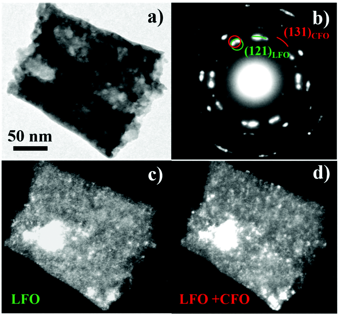Fig. 5 Sample S4′: (a) TEM bright field image, (b) corresponding SAED pattern, (c) dark field image highlighting the presence and distribution of LFO nanocrystals, and (d) dark field image highlighting the presence and distribution of LFO and CFO nanocrystals.

3.2. Magnetization measurements

3.2.1. Magnetic coupling in nanocomposites: effect of synthesis method. In Fig. 6, we show the magnetic field-dependent magnetization loops of all the LFO–CFO nanocomposites (S1–S4) recorded at T = 5 K. At a first glance, the magnetic behavior of the samples S1–S3 look remarkably similar, at least qualitatively, while S4 shows a somewhat different behavior. This is confirmed by a quantitative analysis of the magnetization loops that reveals coercivity (H_C) values of 0.35 T, 0.25 T, 0.28 T, and 0.63 T, and squareness ratios (M_r/M_(5T), where M_r = remanent magnetization and M_(5T) = magnetization at H = 5 T) of 0.4, 0.4, 0.4, and 0.2 for S1, S2, S3, and S4, respectively. We note here that S4 exhibits a larger value of H_C and a smaller squareness ratio, as well as a more open loop compared to the other three samples. The exact reason for this is still under investigation, but could be related to the fact that for S4 the two phases grow simultaneously, while pre-synthesized CFO particles were used for preparing samples S1, S2, and S3. Our preliminary investigation reveals that growing the two phases simultaneously, as in S4, could lead to unique orientation relationships between the two phases that do not exist in the other samples, and this could cause the hysteresis loop of S4 to have a different shape. However, a complete understanding of this requires further study, and is planned for the future. The magnetic field-dependent magnetization of the pure phases (LFO, CFO, and CZFO) are shown in the ESI (Fig. S4†).

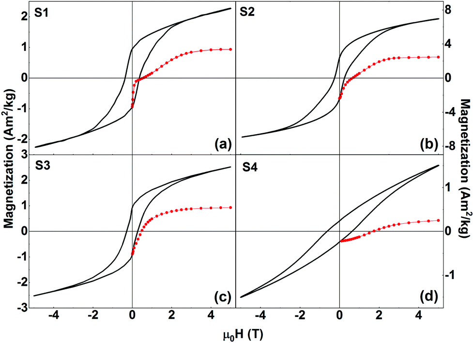Fig. 6 Isothermal field-dependent magnetization loops (black lines) and M_DCDversus reverse magnetic field (red symbols) of (a) S1, (b) S2, (c) S3, and (d) S4 recorded at T = 5 K.

We first investigate the magnetic behavior of samples S1, S2, and S3 in more detail. The apparent qualitative (i.e., shape of the hysteresis loop) and quantitative (values of H_C and squareness ratio) similarities in the M vs. H curves might indicate that the samples exhibit the same physical properties irrespective of the widely differing synthesis methods that were used to prepare these three samples. To check whether this is indeed true, we have performed additional measurements, specifically, direct current demagnetization (DCD) experiments.³⁸ The DCD curve is obtained by first saturating the sample in a negative field (−5 T), and then measuring the remanent magnetization after applying and switching off reverse (positive) fields of increasing amplitude up to H = +5 T. The M_DCDversus reverse magnetic field for each of the nanocomposite samples is also shown in Fig. 6 (red symbols). The M_DCDversus reverse magnetic field for the pure phases (LFO, CFO, and CZFO) are shown in the ESI (Fig. S4†). This measurement protocol allows us to investigate the irreversible process of magnetization. In general, M_DCD lies outside the hysteresis loop. In S1, we observe an anomalous behavior where the initial part of M_DCD lies inside the hysteresis loop. The exact cause of this anomalous behavior is presently unknown and requires more study. This is, however, out of the scope of the present paper.

The differentiated curve of M_DCD with respect to H represents the irreversible component of the susceptibility (χ_irr). This quantity can be considered to be a measure of the energy barrier distribution which, in a nanoparticle system, is associated to the distribution of particle's switching field, defined as the field necessary to overcome the energy barrier during an irreversible reversal process.³⁹ In Fig. 7a, we show the switching field distributions (SFDs) of the nanocomposites as obtained from the first order derivatives of the M_DCD curves. The curves have been normalized for easy comparison.

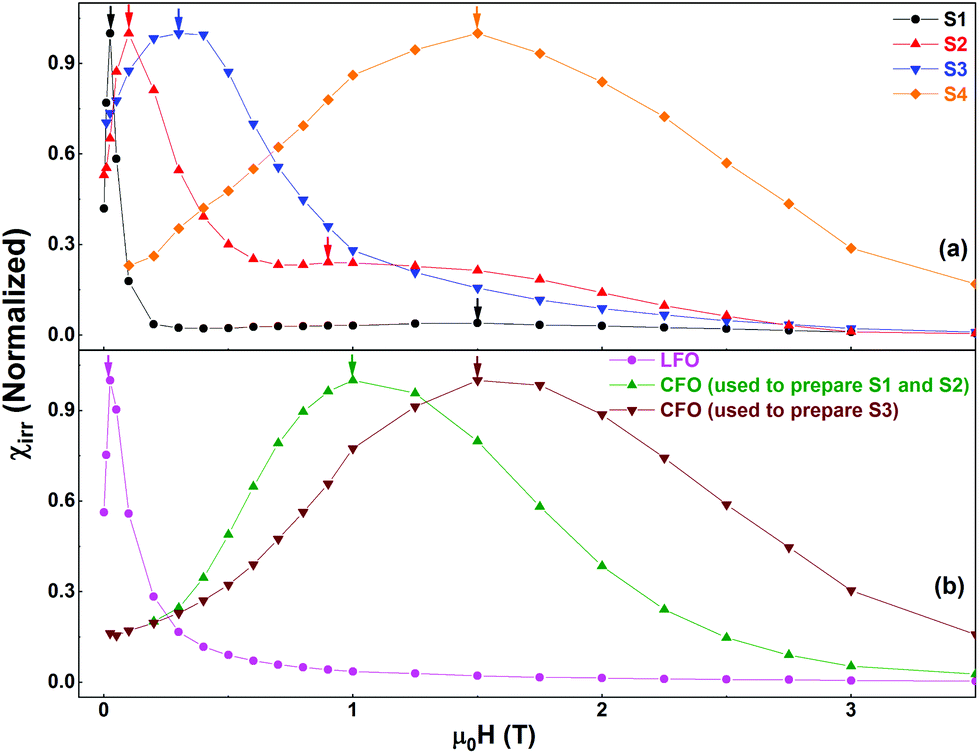Fig. 7 Switching field distributions of (a) S1, S2, S3, and S4 and (b) the pure phases as obtained from the first order derivatives of the corresponding M_DCD curves.

Fig. 7b shows the normalized χ_irr plots for the pure phases. The SFD of S1 presents a strong contribution centered at a low field (∼0.025 T), and a weak signal at a high field (∼1.5 T), shown by the two black arrows in Fig. 7. These can be attributed to the reversal processes of the two individual phases (LFO and CFO), without any sign of a clear coupling. The second peak at ∼1.5 T is clearly visible when the y-axis is plotted in a log scale (see Fig. S5 in the ESI†). In contrast, in S2, the contributions of the pure phases are visible, but the two average switching fields have shifted closer to each other with respect to S1 (shown by the two red arrows in Fig. 7a). This shift indicates the presence of magnetic coupling between the two phases, since the reversal of the two magnetic phases is not independent.³⁸ In S3, the individual contributions of the two phases cannot be distinguished anymore. A single peak is observed (indicated by the blue arrow in Fig. 7a), indicating a single average switching field, and thus, an increase in the magnetic coupling as compared to that in S2. From a physical point of view, the increase in the magnetic coupling as we move from S1 to S3 can be understood as follows. S1 was prepared using simple physical mixing, and hence the magnetic coupling between the two phases is expected to be the weakest (nearly non-existent). S2 and S3 are both prepared using chemical routes, and hence, the magnetic coupling in these two samples is stronger than that in S1. However, S2 was prepared using larger CFO nanoparticles that are relatively aggregated, while S3 was prepared using well-dispersed CFO nanoparticles. Thus, the two phases are much more evenly distributed in S3, while S2 can still contain clusters of the individual phases. Hence, the magnetic coupling in S3 is stronger than that in S2.

Next, we explore the magnetic behavior of S4. For the synthesis of this sample, we did not use any pre-formed phase. Rather, the two individual phases of the nanocomposite were formed at the same time during the synthesis process. Thus, we expect a good dispersion between the two phases, and hence a very good magnetic coupling between them. Indeed, the SFD of this sample shows a single peak i.e., a single average switching field (Fig. 7a), similar to what was observed in S3. However, the average switching field of the two samples (S3 and S4) show more than one order of magnitude difference (indicated respectively by the blue and orange arrows in Fig. 7a). We also note that the average switching field observed in S4 is very similar to that of the 5 nm, well-dispersed CFO nanoparticles (brown curve in Fig. 7b). We believe that the reason for this is that during the synthesis of S4, the CFO phase grows within the LFO phase, and the latter restricts the growth of CFO. To confirm this, we have prepared an additional sample (S4′′) using the same procedure used for S4 but with LFO : CFO = 50 : 50. The reason for preparing a new sample is that the % of CFO in S4 is too low to be detected in its XRPD pattern. The XRPD pattern of S4′′ is shown in Fig. S6a in the ESI.† A comparison of the peak width of the strongest reflection (∼35.5°) corresponding to CFO in this sample with that of the strongest reflection in the XRPD pattern of CFO (inset of Fig. S6b†) proves that the particle size of CFO in the nanocomposite is smaller than that in CFO, as reflected by the larger peak width in the XRPD pattern of the nanocomposite compared to that of CFO (inset of Fig. S6b†). Thus, even though the final annealing temperature is the same for the samples S2, S3, and S4, the crystallite size of CFO is smaller in S4 as compared to that in S2 and S3. In other words, in S4, the matrix (LFO) has a profound effect on the CFO phase, and hence, on the resultant nanocomposite.

3.2.2. Magnetic coupling in nanocomposites: effect of magnetic anisotropy. In S4, the CFO phase was tuned by the effect of the matrix. In the last sample that we have studied i.e., S3′, we explore what happens when the magnetic anisotropy of the CFO phase is tuned by doping. Thus, we used 5 nm, well-dispersed Co_0.5Zn_0.5Fe₂O₄ (CZFO) nanoparticles to prepare an LFO–CZFO nanocomposite sample (S3′). We note that the purpose here is not to perform a systematic tuning of the magnetic anisotropy of CFO by Zn-doping, which was already reported in one of earlier publications.³⁰ Nevertheless, including sample S3′ in the current study allows us to show that our method of estimating the magnetic coupling using demagnetization experiments works not only for the specific case of LFO–CFO, but also when the magnetic anisotropy of the second phase is changed by elemental doping.

In the inset of Fig. 8, we show the isothermal field-dependent magnetization loop and M_DCDversus reverse magnetic field (black line and red symbols, respectively) of S3′. H_C and squareness ratio of this sample are 0.16 T and 0.4, respectively. In the main panel, we show the SFDs of S3′ along with those of the individual pure phases. As in S3 (prepared using the same synthesis route), we see a single peak i.e., a single average switching field in the χ_irr plot of S3′. The effect of tuning the anisotropy of CFO (by doping Zn at the Co-site in CFO) is evident. The average switching field of S3′ is lower than that of S3, since the average switching field of CZFO is lower than that of CFO.

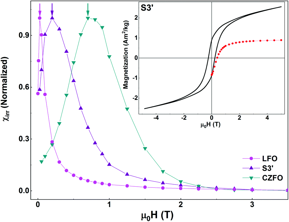Fig. 8 Inset: Isothermal magnetization curve (black line) and M_DCDversus reverse magnetic field (red symbols) of S3′ recorded at T = 5 K. Main panel: Switching field distributions of S3′, LFO, and CZFO as obtained from the first order derivatives of the corresponding M_DCD curves.

4. Conclusions

In summary, we have synthesized LaFeO₃–CoFe₂O₄ (LFO–CFO) and LaFeO₃–Co_0.5Zn_0.5Fe₂O₄ (LFO–CZFO) nanocomposites using different synthesis techniques, and made an estimation of the magnetic coupling in them. While the nanocomposites show apparent similarities in their M vs. H curves, more advanced dc demagnetization measurements reveal striking and very important differences in magnetic coupling in the systems. These differences can be traced back to the differences in the synthesis techniques that dictate the degree of particle agglomeration in the samples. This work shows how the degree of particle agglomeration can be used as a tool to control the strength of magnetic coupling in nanocomposites. Changing the degree of particle agglomeration allows us to tune the surface area of contact between the two phases; in particular, by decreasing the degree of agglomeration, we are able to increase the surface area of contact between the two phases. Thus, by modifying the synthesis approach, we are able to maximize the contact area between CFO and LFO in S4, thus, increasing the interaction both in case of dipolar coupling or direct exchange. These results, illustrated using two prototypical systems (LFO–CFO and LFO–CZFO), are representative of a much more general trait in magnetic nanocomposites where the degree of agglomeration is inversely related to the surface area of contact between the two phases, and hence, to the extent of magnetic coupling. We note, however, that the degree of particle agglomeration might not be the only intrinsic factor influencing the strength of magnetic coupling. Other factors like morphology and shape of the nanocrystals that can influence the surface area of contact between the two phases might also play a key role, and should be investigated in future studies. Finally, our results bring out the importance of careful and detailed magnetic measurements to uncover physical effects that might remain hidden and undiscovered in more conventional measurement protocols.

Conflicts of interest

There are no conflicts of interest to declare.

Acknowledgements

We thank Carl Tryggers Stiftelse för Vetenskaplig Forskning (grant number KF 17:18), Swedish Research Council (including VR starting grant number: 2017-05030), Stiftelsen Olle Engkvist Byggmästare (grant number: 188-0179), and the Royal Physiographic Society of Lund (the Märta and Eric Holmberg Endowment) for financial support. SJ thanks the Ministry of Higher Education, Science and Technology of the Republic of Slovenia (grant no. P2-0091), Slovenian Research Agency (grant no. J2-8169), and the Ministry of Education, Science and Technological Development of Republic of Serbia (Project III45006). We also thank M. Venkata Kamalakar for useful insights.

References

1. A. K. Hauser, R. J. Wydra, N. A. Stocke, K. W. Anderson and J. Z. Hilt, J. Controlled Release, 2015, 219, 76–94.
2. M. B. Gawande, Y. Monga, R. Zboril and R. K. Sharma, Coord. Chem. Rev., 2015, 288, 118–143.
3. D. K. Yi, S. S. Lee and J. Y. Ying, Chem. Mater., 2006, 18, 2459–2461.
4. K. Kan-Dapaah, N. Rahbar, A. Tahlil, D. Crosson, N. Yao and W. Soboyejo, J. Mech. Behav. Biomed. Mater., 2015, 49, 118–128.
5. S. Kalia, S. Kango, A. Kumar, Y. Haldorai and R. Kumar, Colloid Polym. Sci., 2014, 292, 2025–2052.
6. S. H. Hussein-Al-Ali, M. E. El Zowalaty, M. Z. Hussein, M. Ismail, D. Dorniani and T. J. Webster, Int. J. Nanomed., 2014, 9, 351–362.
7. B. H. McDonagh, G. Singh, S. Hak, S. Bandyopadhyay, I. L. Augestad, D. Peddis, I. Sandvig, A. Sandvig and W. R. Glomm, Small, 2016, 12, 301–306.
8. Y. Li, T. Jing, G. Xu, J. Tian, M. Dong, Q. Shao, B. Wang, Z. Wang, Y. Zheng, C. Yang and Z. Guo, Polymer, 2018, 149, 13–22.
9. S. Villa, V. Caratto, F. Locardi, S. Alberti, M. Sturini, A. Speltini, F. Maraschi, F. Canepa and M. Ferretti, Materials, 2016, 9, 771.
10. M.-S. Cao, X.-X. Wang, M. Zhang, J.-C. Shu, W.-Q. Cao, H.-J. Yang, X.-Y. Fang and J. Yuan, Adv. Funct. Mater., 2019, 29, 1807398.
11. Y. Li, W.-Q. Cao, J. Yuan, D.-W. Wang and M.-S. Cao, J. Mater. Chem. C, 2015, 3, 9276–9282.
12. Y. Li, X. Fang and M. Cao, Sci. Rep., 2016, 6, 24837.
13. H. Gu, H. Zhang, J. Lin, Q. Shao, D. P. Young, L. Sun, T. D. Shen and Z. Guo, Polymer, 2018, 143, 324–330.
14. E. Dagotto, Science, 2005, 309, 257–262.
15. T. Sarkar, B. Ghosh and A. K. Raychaudhuri, Phys. Rev. B: Condens. Matter Mater. Phys., 2008, 77, 235112.
16. T. Sarkar, A. K. Raychaudhuri and T. Chatterji, Appl. Phys. Lett., 2008, 92, 123104.
17. T. Sarkar, A. K. Raychaudhuri, A. K. Bera and S. M. Yusuf, New J. Phys., 2010, 12, 123026.
18. T. Sarkar, M. V. Kamalakar and A. K. Raychaudhuri, New J. Phys., 2012, 14, 033026.
19. D. Lahiri, S. Khalid, T. Sarkar, A. K. Raychaudhuri and S. M. Sharma, J. Phys.: Condens. Matter, 2012, 24, 336001.
20. L. Pagliari, M. Dapiaggi, F. Maglia, T. Sarkar, A. K. Raychaudhuri, T. Chatterji and M. A. Carpenter, J. Phys.: Condens. Matter, 2014, 26, 435303.
21. G. Muscas, P. A. Kumar, G. Barucca, G. Concas, G. Varvaro, R. Mathieu and D. Peddis, Nanoscale, 2016, 8, 2081–2089.
22. T. Sarkar, G. Muscas, G. Barucca, F. Locardi, G. Varvaro, D. Peddis and R. Mathieu, Nanoscale, 2018, 10, 22990–23000.
23. M. Bibes and A. Barthélémy, Nat. Mater., 2008, 7, 425–426.
24. W. C. Koehler and E. O. Wollan, J. Phys. Chem. Solids, 1957, 2, 100–106.
25. N. T. Thuy and D. L. Minh, Adv. Mater. Sci. Eng., 2012, 1155(380306), 1–6.
26. W.-Y. Lee, H. J. Yun and J.-W. Yoon, J. Alloys Compd., 2014, 583, 320–324.
27. S. Phokha, S. Pinitsoontorn, S. Maensiri and S. Rujirawat, J. Sol-Gel Sci. Technol., 2014, 71, 333–341.
28. S. Acharya, J. Mondal, S. Ghosh, S. K. Roy and P. K. Chakrabarti, Mater. Lett., 2010, 64, 415–418.
29. J. W. Seo, E. E. Fullerton, F. Nolting, A. Scholl, J. Fompeyrine and J.-P. Locquet, J. Phys.: Condens. Matter, 2008, 20, 264014.
30. V. Mameli, A. Musinu, A. Ardu, G. Ennas, D. Peddis, D. Niznansky, C. Sangregorio, C. Innocenti, N. T. K. Thanh and C. Cannas, Nanoscale, 2016, 8, 10124–10137.
31. J. F. Scott, Nat. Mater., 2007, 6, 256–257.
32. E. E. Ateia, M. K. Abdelamksoud and M. A. Rizk, J. Mater. Sci.: Mater. Electron., 2017, 28, 16547–16553.
33. V. M. Gaikwad and S. A. Acharya, RSC Adv., 2015, 5, 14366–14373.
34. C. Cannas, A. Falqui, A. Musinu, D. Peddis and G. Piccaluga, J. Nanopart. Res., 2006, 8, 255–267.
35. C. Cannas, A. Musinu, D. Peddis and G. Piccaluga, J. Nanopart. Res., 2004, 6, 223–232.
36. S. Jovanovic, M. Spreitzer, M. Trams, Z. Trontelj and D. Suvorov, J. Phys. Chem. C, 2014, 118, 13844–13856.
37. G. K. Williamson and W. H. Hall, Acta Metall., 1953, 1, 22–31.
38. A. López-Ortega, M. Estrader, G. Salazar-Alvarez, A. G. Roca and J. Nogués, Phys. Rep., 2015, 553, 1–32.
39. D. Peddis, P. E. Jönsson, S. Laureti and G. Varvaro, Front. Nanosci., 2014, 6, 129–188.

---

Footnote

† Electronic supplementary information (ESI) available. See DOI: 10.1039/c9nr05364f

---