
An Ising transition of chessboard tilings in a honeycomb liquid crystal†
William S.
Fall
 ac,
Constance
Nürnberger
b,
Xiangbing
Zeng
*d,
Feng
Liu
a,
Stephen J.
Kearney
c,
Gillian A.
Gehring
*c,
Carsten
Tschierske
*b and
Goran
Ungar
*ad
ac,
Constance
Nürnberger
b,
Xiangbing
Zeng
*d,
Feng
Liu
a,
Stephen J.
Kearney
c,
Gillian A.
Gehring
*c,
Carsten
Tschierske
*b and
Goran
Ungar
*ad
aState Key Laboratory for Mechanical Behaviour of Materials, School of Materials Science & Engineering, Xi'an Jiaotong University, Xian 710049, China
bDepartment of Chemistry, Martin Luther University Halle-Wittenberg, Kurt-Mothes-Str. 2, 06120 Halle, Germany. E-mail: carsten.tschierske@chemie.uni-halle.de
cDepartment of Physics and Astronomy, University of Sheffield, Sheffield S3 7RH, UK. E-mail: g.gehring@sheffield.ac.uk
dDepartment of Materials Science and Engineering, University of Sheffield, Sheffield S1 3JD, UK. E-mail: x.zeng@sheffield.ac.uk; g.ungar@sheffield.ac.uk
First published on 29th January 2019
Abstract
We have designed a compound that forms square liquid crystal honeycomb patterns with a cell size of only 3 nm and with zero in-plane thermal expansion. The compound is a bolaamphiphile with a π-conjugated rod-like core and two mutually poorly compatible side-chains attached on each side of the rod at its centre. The system exhibits a unique phase transition between a “single colour” tiling pattern at high temperatures, where the perfluoroalkyl and the carbosilane chains are mixed in the square cells, to a “two-colour” or “chessboard” tiling where the two chain types segregate in their respective cells. Small-angle transmission and grazing incidence X-ray studies (SAXS and GISAXS) indicate critical behaviour both below and above the transition. Both phase types are of considerable interest for sub-5 nm nanopatterning. The temperature dependence of ordering of the side chains has been investigated using Monte Carlo (MC) simulation with Kawasaki dynamics. For a 3-dimensional system with 2 degrees of freedom, universality predicts that the transition falls into the 3d Ising class; MC was therefore used to calculate observables and determine the critical exponents accessible in experiment. Theoretical values of ν, γ and, perhaps most importantly, of the order parameter β have been calculated and then compared with those determined experimentally. β found experimentally is close to the theoretical value, but ν and γ values are significantly smaller than predicted. To explain the latter, the measured susceptibility above Tc is compared with those from simulations of different lattice sizes. The results suggest that the discrepancies result from a reduced effective domain size, possibly due to kinetic suppression of large scale fluctuations.
Design, System, ApplicationFor surface patterning on a sub-10 nm scale, self-assembling columnar liquid crystals with 2d long-range periodicity, are the natural choice. For application in nano-electronics, the pattern should ideally be square and have zero in-plane thermal expansivity. Moreover, it may be desirable to add a degree of complexity in the pattern, such as producing a “chessboard” pattern with alternative squares chemically different thus, e.g. combining alternating p- and n-semiconducting pathways, or electronically and ionically conducting channels, or similar. This report shows how such a system can be achieved in principle, based on an inverse columnar phase where a bistolane rod-like core provides a fixed-sized square honeycomb framework held together by H-bonding glycerol end-groups. The prismatic cells are filled alternately by a semiperfluorinated (F) and a carbosilane (Si) chain, respectively attached to either side of the linear core. The chessboard structure with 3 nm alternating square cells is achieved through an appropriate choice of the core length, side-chain area to core length ratio, and the level of incompatibility between the side-chains, as detailed in the Introduction. |
Introduction
Among numerous well established or developing applications of liquid crystals (LC) is nanoscale patterning on the sub-10 nm length scale.1,2 Such patterning may be used in organic electronics and photovoltaics,3–8 in selective membranes,9–11 for ion conducting arrays,12,13 cubosomes14 and hexosomes15 for drug delivery etc. For use in soft nanolithography highly ordered arrays are required, preferably with a square or rectangular lattice and high dimensional stability, ideally with zero thermal expansion. Self-assembled square arrays with high order have been achieved using block copolymers, but not on a sub-10 nm scale.16 Columnar LC phases are an obvious choice for sub-10 nm and even sub-5 nm arrays. But the conventional columnar phases, with an aromatic column core and a peripheral corona of flexible, most often aliphatic chains, usually have hexagonal symmetry.17,18 Rectangular columnar phases are not rare, but typically they are centred (plane group c2mm), meaning that they are again just distorted hexagonal arrays. Square columnar phases are exceptions.19,20 Even compounds with a square molecular shape mainly form hexagonal lattices, because the soft aliphatic corona allows rotational averaging around the column axis.Promising and already extensively studied bolaamphiphiles consisting of a polyaromatic rod-like core, H-bonding end-groups and laterally attached flexible chains, have shown great versatility in forming a range of “inverted” columnar LC phases, i.e. honeycombs with aromatic walls (the “wax”) and the side-chains as cell fillers (the “honey”).21–24 These honeycomb networks prevent rotational averaging. The number of sides in the polygonal cross-section of a prismatic cell (the “tile”) is determined by the ratio between the area of the filler side-chains to the length of the rod-like core. Normally the side length of the polygon equals the length of the molecule, although in some cases double-length sides were found containing two end-linked rods.25,26 A range of tiling patterns have been obtained in this way, from simple triangular to highly complex nanopatterns containing up to five different coexisting tile types.27 Square patterns were, however, only found under special circumstances in a small temperature range.21,28E.g., Recently, several members of a series of terphenyl-based bolaamphiphiles were found to exhibit non-centred (p2mm) rectangular lattices; however the cell aspect ratio was highly temperature sensitive, reaching 1![[thin space (1/6-em)]](https://www.rsc.org/images/entities/char_2009.gif) :1 (square lattice) only close to isotropization temperature.29
:1 (square lattice) only close to isotropization temperature.29
Beside their application potential, LCs are of considerable scientific interest, providing soft matter and low-dimensional equivalents to phenomena such as phase transitions, extensively studied in more traditional areas of condensed matter physics. Well known examples include the nematic to smectic-A transition30 and the twist-grain-boundary (TGB) smectic phase,31 both having their analogue in superconductivity, as well as the hexatic smectics being easily accessible examples of 2D melting phenomena.32 Ferro-, ferri- and antiferroelectric chiral smectics33 and the currently topical twist-bend nematic phase34,35 are further examples of new states of condensed matter. In contrast to numerous studies of phase transitions in nematics and smectics, transitions in thermotropic LCs with two-dimensional order have been investigated in only a few cases experimentally36–38 or by theory and simulation.27,39–44
In the LC square patterns previously reported all squares were uniform. In order to increase functionality, the combinations of different squares, filled with different materials would be required. For this purpose a change in molecular design was required, whereby the single lateral alkyl chain of the above-mentioned terphenyls is replaced by two different and incompatible chains at the two opposite sides of the rod-like unit. The incompatibility between perfluorinated alkyl chains and hydrocarbon chains45 is a successfully employed approach to obtaining multicolour tiling patterns.24,25 However, in order to achieve adequate incompatibility the number of CH2 and CF2 units must be sufficiently large for the demixing energy to overcome the entropy penalty. However, these longer chains require more space in the prismatic cells. In order to retain square cells, the terphenyl cores forming the honeycomb were extended by the incorporation of additional ethynyl units between the benzene rings. Furthermore, in order to lower the crystal melting point, a highly branched carbosilane unit was used instead of a linear alkyl chain. The introduction of silicon as branching points into a hydrocarbon chain allows a synthesis in fewer steps than would be required for similarly branched hydrocarbons.
Here we report the self-assembly of a new LC system, formed by a bolapolyphile with a 1,4-bis(phenylethynyl) benzene (“bistolane”) core45 with two disparate chains attached laterally to the 2 and 5 positions (compound 1, Scheme 1).
 | ||
| Scheme 1 Compound 1 and its transition temperatures (Cr = crystal, Colsq2 = two-colour square columnar phase, Colsq1 = single-colour square columnar phase, Iso = isotropic liquid). | ||
As will be shown in the following sections, this compound is found to form a square honeycomb with exceptional dimensional stability. Moreover it displays a disorder–order transition from a uniform square tiling to a two-colour chessboard-type tiling where the two side-chains segregate in separate square cells. The transition is thought to be a close real life example of the well-known and widely studied Ising model of magnetic spins.46 Monte Carlo simulations show the critical behaviour (e.g. development of short range fluctuations and long range order around the phase transition temperature), observed by X-ray diffraction, to closely match the 3D Ising model on both sides of the transition, provided the finite domain size is taken into account.
Experimental results
The synthesis of compound 1 was performed by Sonogashira coupling as the key steps45 as described in the ESI.† Polarized optical microscopy (POM) images (Fig. 1 and S1†) show birefringent textures with frequent fan shapes. In fact large areas of the images remain black (Fig. 1a and c) indicating that the mesophase is optically uniaxial with the optic axis perpendicular to the glass surface (homeotropic alignment). The birefringence persists up to 132 °C. Differential scanning calorimetry (DSC) shows a weak melting endotherm on second heating around 70 °C, and a sharp isotropization peak at 132 °C, transition enthalpy 5.6 J g−1 (Fig. S2†). The latter transition shows very little hysteresis on cooling, while crystallisation is completely suppressed at the cooling rate used (10 K min−1).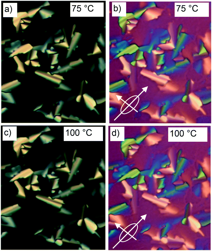 | ||
| Fig. 1 Optical micrographs of compound 1 between crossed polarizers recorded at (a and b) 75 °C and (c and d) 100 °C. Images b and d were recorded with an additional λ retarder plate, whose indicatrix orientation is depicted in the images. The field-of-view width is 0.1 mm. | ||
Powder small-angle X-ray scattering (SAXS) curves of compound 1 recorded during continuous heating at 0.5 K min−1 are shown in Fig. 2a. The bold trace at Tc = 88 °C marks the phase transition between two square columnar phases. In both phases reflections indexed as (10), (11), (20) etc. are seen, their q2 ratio being 1:2:4:5…. This defines the plane group as p4mm in both cases. Most notable is the decay and eventual disappearance of the strong (10) reflection of the low-T phase at Tc, along with the disappearance of (21) and (30) peaks. On heating above Tc the intensity of the remaining Bragg peaks stays almost unchanged: the (11), (20) and (22) diffraction peaks transit smoothly into the (10), (11) and (20) peaks of the high-T square phase. Remarkably also, the remaining peaks do not shift in the entire range from room temperature to the isotropization temperature Ti.
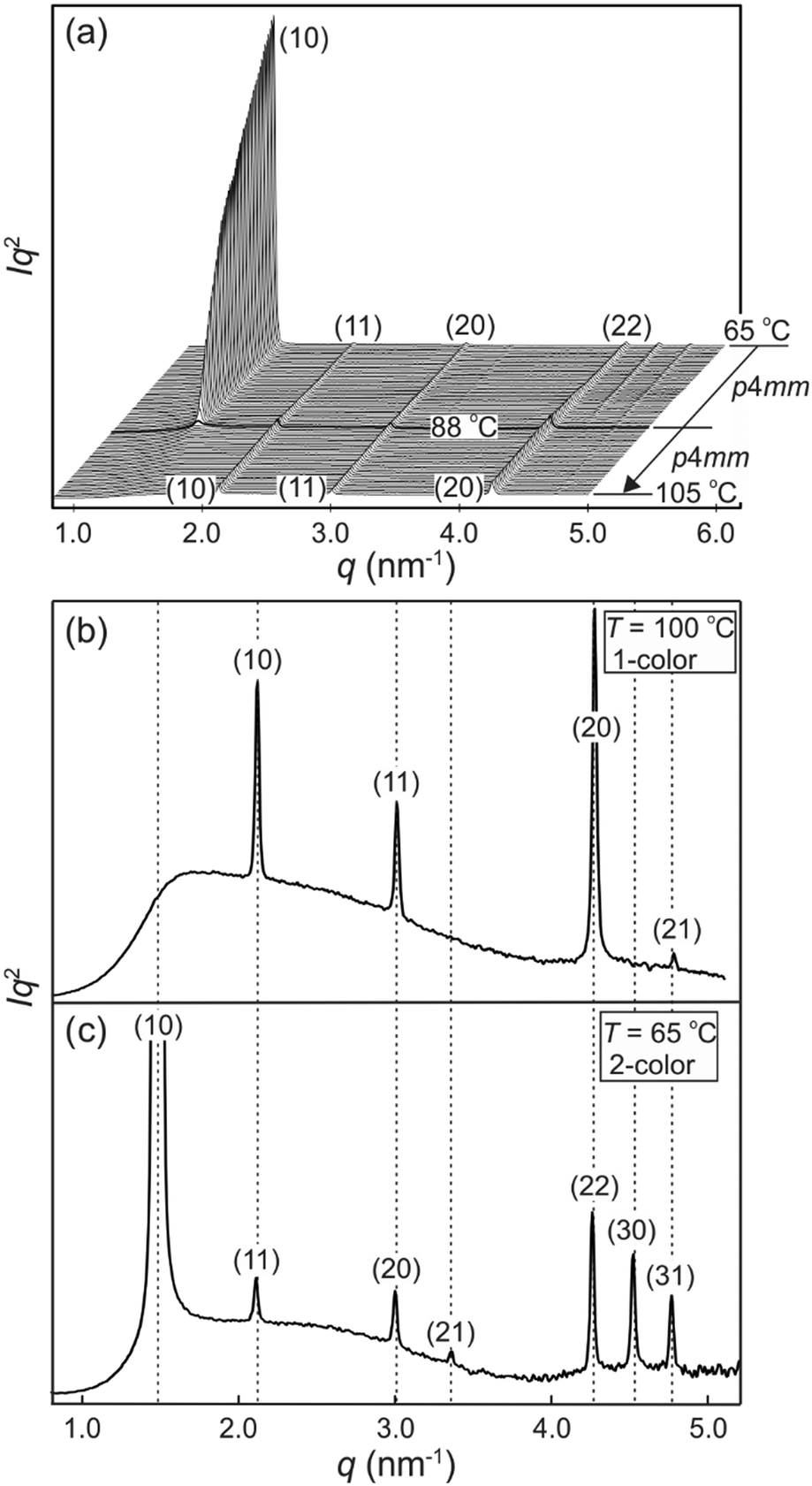 | ||
| Fig. 2 Powder SAXS traces of compound 1. (a) Stacked traces recorded during heating at 0.5 K intervals. The bold curve is recorded at Tc (b and c) SAXS trace of the high-temperature 1-colour square honeycomb phase at 100 °C (b), and of the low-temperature 2-colour chessboard phase recorded at 65 °C. Miller indices (hk) apply to the respective lattices. | ||
The above indexing of the diffraction pattern was also confirmed by grazing incidence SAXS (GISAXS) experiments on a surface-oriented thin film of 1 on silicon substrate, as shown in Fig. 3. Although most of the sample is homeotropic, giving diffraction peaks on the horizon line, off-equatorial reflections are also seen from areas where the columns lie parallel to the surface, rotationally averaged in the film plane. The most notable feature in Fig. 3 is the existence of strong diffuse scattering above Tc in place of the (10) Bragg reflections of the low-T phase – the relationship is highlighted by the light blue lines in Fig. 3. This indicates the persistence of short-range critical electron density fluctuations above Tc, which will be analysed quantitatively further below.
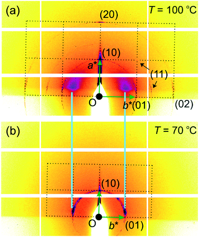 | ||
| Fig. 3 GISAXS pattern of the (a) 1-colour phase and (b) 2-colour phase. Dotted lines indicate the reciprocal lattice applicable to areas with planar columns. The majority of the sample is homeotropic, giving rise to all-equatorial reflections; these are visible in the top pattern (note the (11) arc near the horizon), but not in the bottom one, as these reflections are beyond the horizon because of the slightly higher tilt of the substrate plane relative to the incident beam. | ||
The lattice parameters a1 and a2 of the high- and low-T phases are 2.96 nm and 4.19 nm, respectively. As the ratio is exactly  , the area of the unit cell of the low-T phase is twice that of the high-T phase. Electron density maps, calculated on the basis of relative diffraction intensities and the selected structure factor phases given in Table S1,† are shown in Fig. 4a and c.
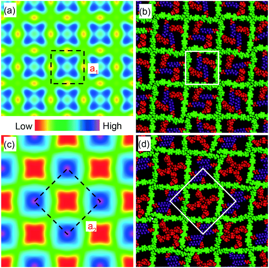 | ||
| Fig. 4 (a and c) Electron density maps of the (a) high-T and (b) low-T phase in the xy plane perpendicular to the columns. The medium-high density squares in (a) (blue) contain a mixture of perfluorinated (F) and carbosilane (S) chains, the blue/purple squares in (c) contain predominantly F chains, while the red squares in (c) contain mainly Si chains. The four dark maxima in each blue square in (a) are believed to be artifacts (“ripples”) due to early truncation of the Fourier series, i.e. due to the small number of measured reflections. (b and d) Snapshots of molecular models after annealing dynamics runs in the (b) high-T and (d) low-T chessboard phase. Colour code: green = π-conjugated core including glycerol end groups (medium electron density), red = alkyl and carbosilane groups (lowest density), purple = perfluoroalkyl groups (highest density). For details of molecular dynamics annealing see Methods. The white squares delineate a unit cell. | ||
Considering the molecular model, we note that a1 = 2.96 nm is very close to the 2.80–3.05 nm length of the molecule, as measured between the ends of the glycerol groups, depending on the glycerol conformation. This, combined with the fact that the high birefringence axis (i.e. the long axis of the π-conjugated molecular core) is perpendicular to the columns (see POM images with a λ retarder plate in Fig. 1b and d and S1c†), strongly suggests the model in Fig. 4b for the high-T phase. Such a model is consistent with the general self-assembly mode of bolapolyphile LC honeycombs, except that a square honeycomb is rather rare. In this structure the cell walls consist of molecular cores lying normal to column axis with each of the two side chains located in the two neighbouring cells. In the high-T phase the cells are filled on average with a 1:1 mixture of F and Si chains. The model in Fig. 4b has been subjected to 30 cycles of molecular dynamics annealing between room T and 700 K lasting 30 ps in total. It shows a reasonable packing density, indicating that the model is feasible. It is also consistent with the electron density map, where the light blue squares reflect the fact that the average electron density of the combined F and Si chain (572 e nm−3) is somewhat higher than that of the bistolane/glycerol core (518 e nm−3) – for details see Table S2.†
The doubling of the unit cell below Tc, the high intensity of the (10) reflection of the low-T lattice, and the reconstructed electron density map in Fig. 4c all suggest that a disorder–order transition takes place at Tc, with the F and Si chains preferentially occupying alternative cells, creating a chessboard tiling as in Fig. 4c and d. In a structure with perfectly segregated Si and F chains, we calculate that the contrast between Si and F cells would be 714–430 = 284 e nm−3, which is >5 times higher than the contrast between the mixed cell interior and the bistolane/glycerol wall. Hence the very much stronger (10) Bragg reflection of the chessboard phase compared to that of its (11) reflection or of the (10) reflection of the high-T phase (note that the intensity scales roughly as square of the electron density contrast).
Theory
The change of symmetry between cells, containing a disordered mix of chains, to a state where there is long range chessboard order is analogous to that of interacting Ising spins. In the model adopted here (Fig. 5) the orientation of the side chains can only take one of two values, allowing only 180° rotational jumps of the molecules around their terphenyl axes. These are equivalent to spin flips in the original magnetic model. Intermediate states are disallowed, and the energy of each cell of the system depends only on the types of side chain therein. A molecular flip alters the balance between the numbers of perfluoroalkyl and carbosilane chains in the two adjoining cells. Dynamics in which this spin or molecular ‘flipping’ impacts both neighbouring configurations is known as Kawasaki Dynamics. While the symmetry of the system changes abruptly at the transition temperature or critical temperature (Tc), a particular physical property (e.g. order parameter) of the system changes continuously above or below the transition, and depends on some power of the magnitude of the temperature difference to the transition temperature; this power is known as a critical exponent.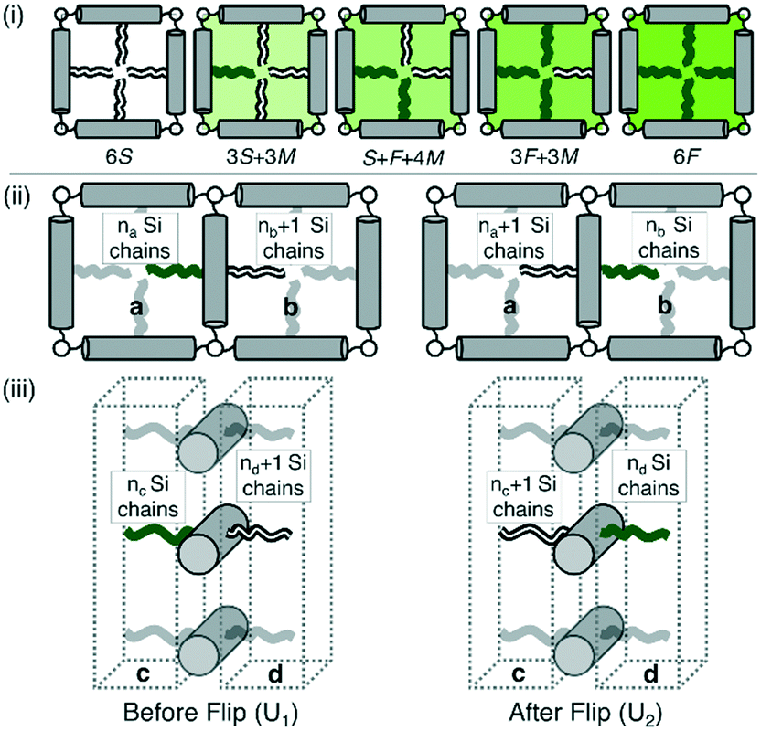 | ||
| Fig. 5 (i) Allowed configurations of the square tiles and their associated energies in terms of pair interactions S, F and M (see Table 1) (ii) in plane interactions: the configurations 1 and 2 of a chain in the fully ordered state that is flipped between squares a and b. Square a contains na Si chains and 3 − na F chains, similarly for b. (iii) Out of plane interactions: the configurations 1 and 2 of a chain in the fully ordered state that is flipped between columnar interaction regions c and d. Region c contains nc Si chains and 2 – nc F chains, similarly for d. | ||
Since both the dimensionality and degrees of freedom are the same, by universality, it is sensible to conclude that the model should have the critical exponents of the 3d Ising universality class. A simple lattice model has been devised and MC simulation is used to test this conjecture. The theoretical values for the critical exponents are determined and compared with experimental values in the sections that follow. It is interesting to note that due to the introduction of pairwise interactions, we conclude that there is only one significant energy in this problem; that is the energy difference between like attractive and unlike mutually repulsive chains. The ordered states are therefore found to be exactly symmetric. Any one molecule contains one chain of each type hence flipping a molecule changes the energy state of both neighbouring tiles; this is analogous to the 3d Ising model of magnetic spins under Kawasaki spin flip dynamics.
Each LC molecule is comprised of two different side chains one silicone (S) and one fluorine (F) which may pairwise interact. Like interactions are more strongly attractive than unlike interactions which results in an order–disorder transition. Within each supramolecular square the side chains can interact equally through 3 different pair interactions; these are S: Si–Si, F: F–F and M: Si–F. Crucially, chain–chain interactions within a square carry equal weight and the positioning inside the supramolecular square is neglected. The total possible number of interactions which exist in any given square describes the squares energy, that is for n Si chains and (4 − n) F chains the total energy can be expressed as the number of distinct interactions; Si–Si: n(n − 1)/2, F–F: ((4 − n)(3 − n))/2 and Si–F: n(4 − n).
The 5 possible configuration energies for an arbitrary square containing n Si chains and (4 − n) F chains and their multiplicities are given in Table 1. The multiplicities add to 24 = 16 with the largest contribution coming from configuration with an equal number of Si and F chains; indicating the importance of entropy in driving this order–disorder transition.
| No. Si | No. F | Energy | Multiplicity |
|---|---|---|---|
| 4 | 0 | 6S | 1 |
| 3 | 1 | 3S + 3M | 4 |
| 2 | 2 | S + F + 4M | 6 |
| 1 | 3 | 3F + 3M | 4 |
| 0 | 4 | 6F | 1 |
In Fig. 5(i) the configurations before and after a molecule has been flipped on the border between two squares is shown; this is an example of Kawasaki dynamics where the flipping of a single molecule directly changes the energy of both neighbouring squares involved. Interactions between neighbouring molecules out of plane are also included, depicted in Fig. 5(ii); these are taken to be half those in plane. The initial and final configuration energy of the 2 states, U1 and U2 respectively, can be expressed in terms of the pair interactions and number of Si chains in and out of plane
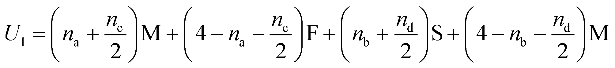 | (1) |
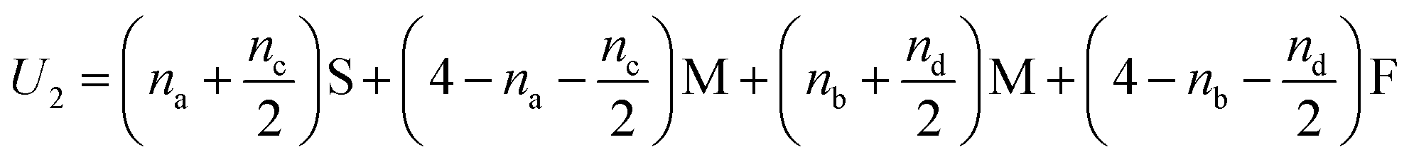 | (2) |
 | (3) |
The constant U0 = [S + F − 2M] is therefore the only significant energy involved in the model since any chain flip affects the chain number in both the neighbouring squares. In our case U0 is always negative because like chains attract more strongly; a chessboard ordering can occur only for negative U0.
Monte-Carlo simulation and critical phenomena
Monte Carlo simulations have been performed on a 3d periodic square lattice for 5 different lattice volumes, 123, 243, 483, 963 and 1923, in order to test the scaling properties and calculate the critical exponents. There are V = 2L3 molecules involved in the simulation for each of the respective lattice volumes. The system employs the Metropolis method,47 in which sample configurations are generated from previous states according to a transition probability. This transition probability is directly proportional to the energy difference, ΔU, between the initial and final states, given by eqn (3). Thus, by calculating the energy ΔU involved for a given molecular ‘flip’ between two neighbouring squares, the Boltzmann weighting can be evaluated at a specified temperature. It is therefore possible to evolve the system and subsequently sample its phase space by accepting or rejecting many flips using random sampling. This is known as the Metropolis algorithm; a molecular ‘flip’ is depicted in Fig. 5 which illustrates the molecular equivalent of Kawasaki dynamics for our system. It is well known that the thermodynamic exponents do not depend on the chosen dynamics i.e. Glauber or Kawasaki.The 3d lattice is broken down into columns of L 2d chessboards each containing two identical sublattices A and B, this is depicted in Fig. 6. A fully ordered 2-colour tiling, (Fig. 6a) consists of alternating columns of supramolecular squares comprising of 4 Si or 4F chains such that the number of Si or F chains in either sublattice is maximised, see Fig. 6b. For a single colour tiling the columns comprise of a mixture of Si or F chains where, on average, the number of Si or F chains in any cell are equal, Fig. 6c and d. The order parameter, σi, for one sample configuration is defined as
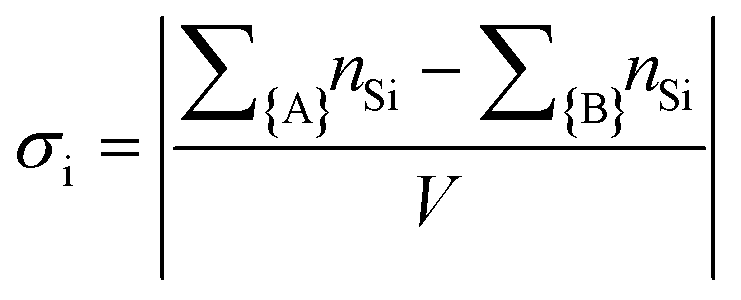 | (4) |
 | (5) |
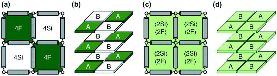 | ||
| Fig. 6 (a) The fully ordered state in terms of 2d squares, (b) fully ordered state in 3d, where the sublattices A and B are indicated, (c) the fully disordered state, (d) the fully disordered state in 3d, where the sublattices A and B are indicated. | ||
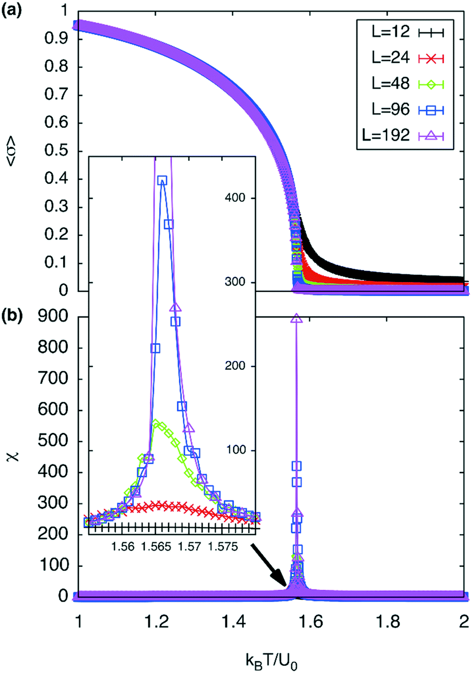 | ||
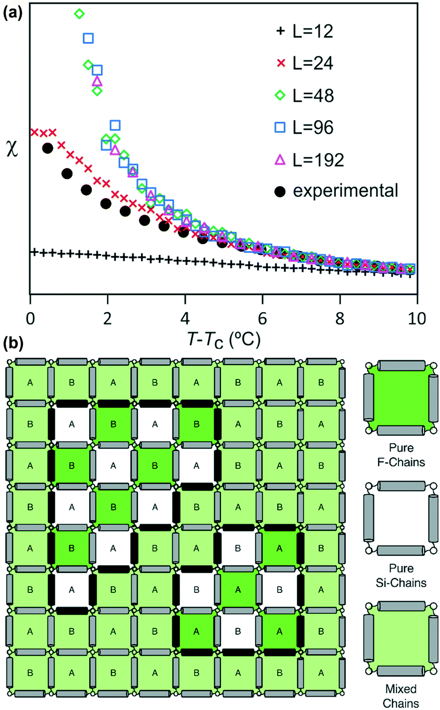
| Fig. 7 (a) Order parameter per square, 〈σ〉, as a function of temperature and (b) susceptibility, χ, as a function of temperature. The inset contains a magnified plot of the susceptibility around Tc showing the effect of finite domain sizes. | ||
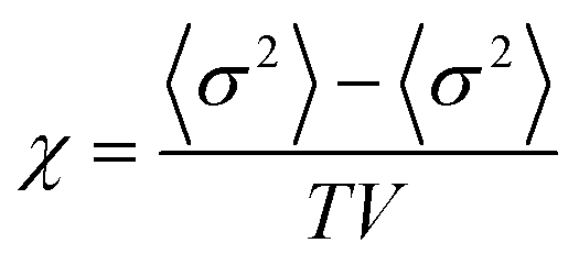
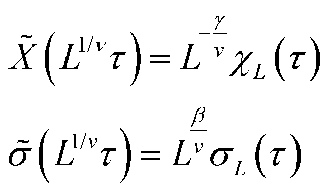
A plot of χ is as a function of temperature is shown in Fig. 7b for 5 different lattice sizes. An initial thermalisation of 104 MC steps is performed and 105 measurements were taken at each temperature. The ensemble averages for the order parameter 〈σ〉 and susceptibility χ are calculated in order to construct the phase diagram. According to universality, the transition should fall into the 3d Ising universality class. By considering the scaling functions for the order parameter, and susceptibility we can confirm this by fitting to the Ising exponents, the scaling functions are given by48
 | (6) |
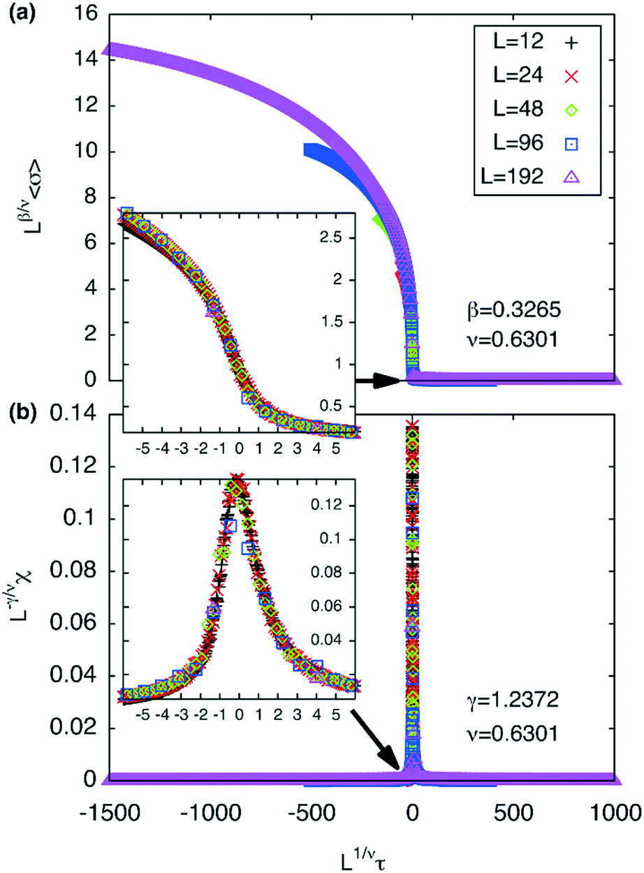 | ||
| Fig. 8 (a) Scaling plot of the order parameter and (b) of the susceptibility. The fit assumes 3d Ising exponents ν = 0.6301, γ = 1.2372 and β = 0.3265 where Tc is taken to be ∼1.5665 kBT/U0.τ (T) = (T − Tc)/Tc. Magnified scaling plots are shown in the inset depicting the data collapse around τ (Tc). | ||
Experimental determination of the critical exponents
The critical exponent β is related to the order parameter (sublattice magnetization) σ, below the transition temperature Tc, by the following relationship| σ = [(Tc − T)/Tc]β | (7) |
We make the assumption that the sublattice magnetization σ is proportional to the amplitude of diffraction, i.e. that the flip of direction of side groups at a side of a square cell (equivalent to a flip of spin), results in a constant increase (or decrease) to the overall structure factor F(10) of the (10) diffraction peak of the two coloured square phase. As the diffraction intensity I(10) is proportional to |F(10)|2, it varies as
| I(10) ∝ (Tc − T)2β | (8) |
The critical exponent β can be found by fitting the diffraction intensity I(10) as a function of temperature to the above equation.
The best-fit to the experimentally determined intensities suggests that 2β = 0.766 and β = 0.383 (Fig. 2a and 9a). This is slightly larger than the value of β = 0.326 expected for a 3d-Ising model and also derived by our Monte Carlo simulation. For comparison, the theoretically predicted curve from the 3d Ising model is shown also in Fig. 9a (broken curve). It is evident that the observed experimental data follows the theoretical curve closely, even though the experimentally observed transition is less sharp than predicted by theory. This slight discrepancy could be attributed possibly to the system not residing in thermal equilibrium, despite the relatively slow heating rate used (0.5 °C min−1).
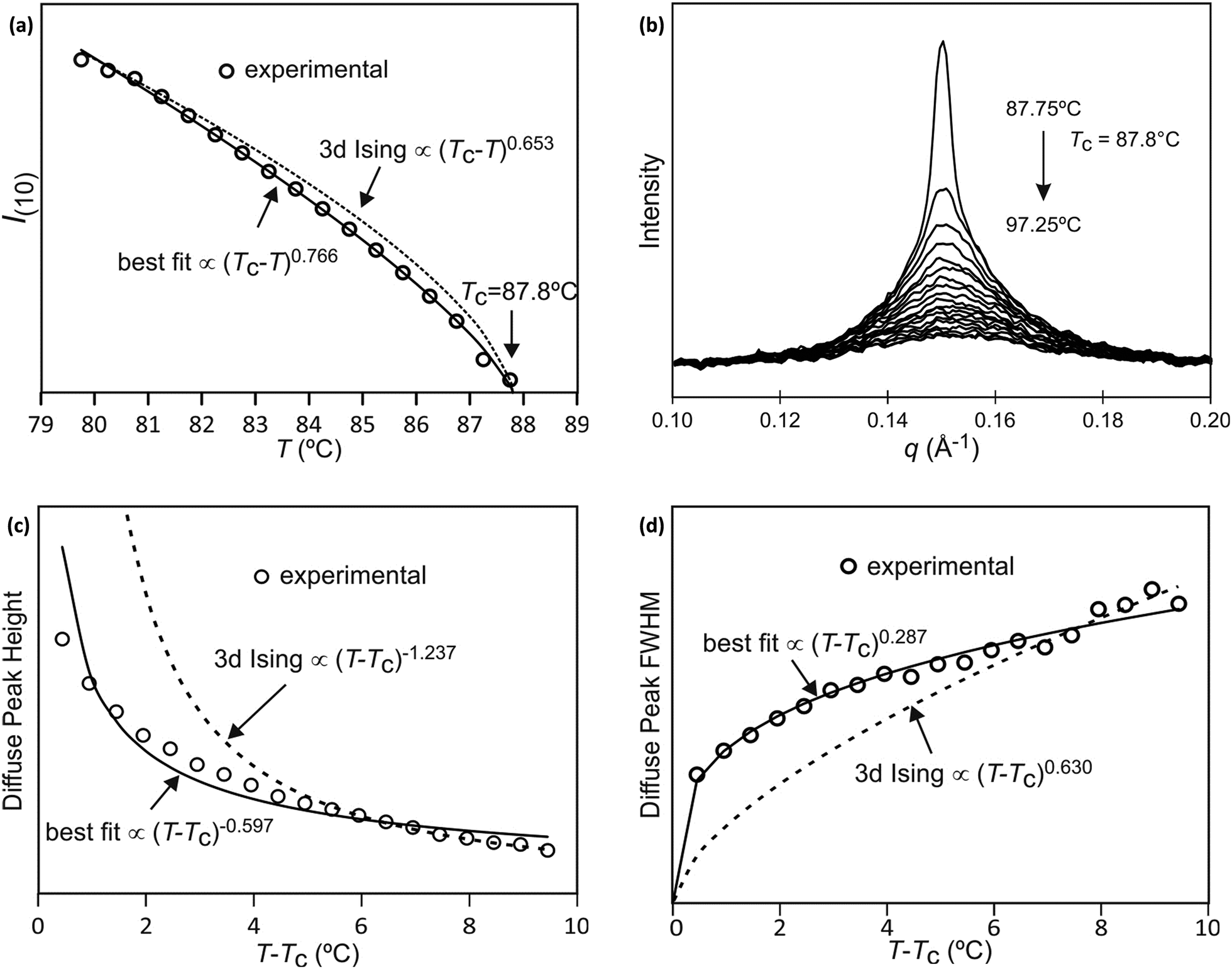 | ||
| Fig. 9 (a) Fitting of I(10) intensity as a function of temperature, (b) Diffuse scattering due to local fluctuation of order parameter, just below and above the critical temperature of Si2F8. Comparison of experimental data, best-fit and theoretical curves of (c) diffuse peak height and (d) FWHM above Tc. | ||
While the change of order parameter below critical temperature carries information of β, two other critical exponents, γ and ν, are related to the local fluctuation-correlation of the order parameter above the critical point, i.e. <σiσj>. Similarly to what has been discussed before, such fluctuations will be reflected in the local fluctuation of structure factor (Fi at lattice point i and Fi proportional to σi) and leads to diffuse scattering, with an intensity proportional to 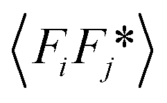 , around q(10). The experimental diffuse scattering peaks just below and above the critical point are shown in Fig. 9b.
For a 3d Ising model, the correlation function G(r) takes the form
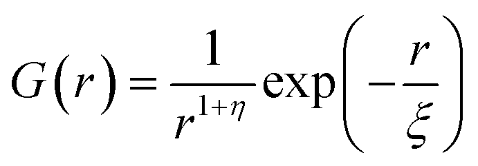 | (9) |
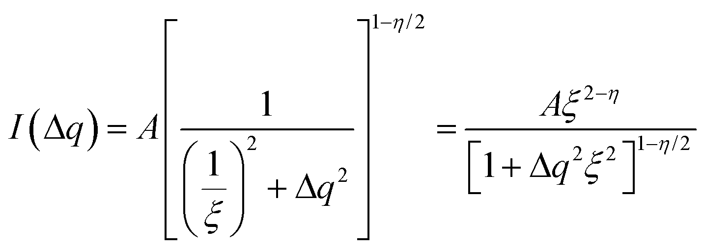 | (10) |
Since for the 3D Ising model critical exponent η is extremely small (0.036), the diffuse peak can be treated as Lorentzian. Therefore, we have fitted the diffuse peaks as shown Fig. 9c and d to a Lorentzian function and retrieved the peak height hD in addition the full width at half maximum (FWHM) values as a function of temperature (Fig. 9, data shown by empty circles). Above the critical point the correlation length ξ is proportional to (T − Tc)−ν. The peak height hD is proportional to the susceptibility χ, and (T −Tc)−γ where γ = (2 − η)ν; and the FWHM = 2/ξ is inversely proportional to the correlation length, therefore50
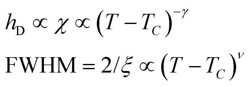 | (11) |
The best-fit and theoretical curves from fitting of peak height and FWHM of the diffuse scattering are compared in Fig. 9.
Discussion
Both best-fit values of γ (0.597) and ν (0.287) are much smaller than the theoretical values: γ should be 1.2372 and ν should be 0.6301. The most evident differences of the experimental diffuse peak to that predicted by theory are found close to the critical temperature: the diffuse peak height is expected to be much higher, while the FWHM is expected to be much smaller i.e. correlation length should be much larger than observed.Such reduction of diffuse peak height or measured susceptibility close to the critical temperature can in fact be seen in our Monte Carlo simulation with different sample sizes (number of cells). Fig. 10a shows the simulated susceptibility for four different domain sizes (123, 243, 483, 963 and 1923 cells respectively), and a significant reduction in the susceptibility close to the critical temperature can be clearly seen for domain sizes of 123 and 243 cells. In fact the trend in the 243 cells is very close to that experimentally observed (Fig. 10a), suggesting a domain size of only ∼70 nm. On the other hand, the width of the (10) Bragg diffraction peak of the two-colour square phase below Tc, and of the (10) peak of the single-colour square phase above Tc, suggest a much larger domain size of ∼250 nm. We speculate that large scale fluctuations of local two-coloured patches are likely to be restricted kinetically, as they involve converting mixed cells at the boundaries of such local patches by exchanging the directions of the two side groups of molecules (Fig. 10b). While in a spin model an inversion of spin has no energy barrier, in our system the corresponding change molecular orientation always has one. Therefore, the chance of large scale fluctuations will be significantly reduced when compared to the situation when no such energy barrier is present. This would result in a smaller effective domain size for the two-colour fluctuations.
 | ||
| Fig. 10 (a) Comparison of experimental and simulated susceptibility, for four different sample sizes with 123, 243, 483, 963 and 1923 cells respectively, above the critical temperature. (b) Local two-coloured fluctuations in the single colour phase above the critical temperature, where A and B label the sublattices. Black molecules mark the domain walls separating the ordered and disordered patches. | ||
Conclusions
We have successfully created a system that self-assembles forming square 2d patterns with a sub-5 nm period. The compound displays two types of square patterns, one simple and another of the chessboard type. The size of the square cells does not change over a 100 K temperature interval, making this type of template eminently suitable for stable nanopatterning. The order–disorder critical transition between the chessboard and simple square phases has been further investigated by Monte Carlo simulation and, as expected, it belongs to the universality class of a 3d Ising model. Good agreement between the experimental and theoretical values of the critical exponent β have been found. While there are apparent discrepancies for critical exponents γ and ν, Monte Carlo simulations suggest that this may result from the reduced effective domain size, as large scale fluctuations above critical temperature are suppressed for kinetic reasons.Having learned the basic nano-architectonic principles of creating 1- and 2-colour square patterns from the above results, in a follow-up study we undertook to increase the cell size. Thus a series of related bolapolyphiles were synthesised, having a longer oligo(p-phenyleneethynylene) core involving five benzene rings instead of only three in the bistolane core and suitably extended side-chains.51 Both, the mixed-chain and the chessboard phases were observed for compounds with appropriate chain lengths, showing that the principles of architectural design learned from the present work are applicable to a wider class of materials and are generic.
Experimental methods
Materials
The syntheses of compound 1 and its intermediates are described in the ESI† together with the analytical data. NMR spectra were recorded with a Varian VXR spectrometer (400 MHz); HR-MS spectra were recorded on Bruker micrOTOF-Q II APPI spectrometer.Polarizing microscopy and DSC
Phase transitions were determined by DSC (DSC-7, Perkin Elmer in 30 μl Al pans) with heating and cooling rates of 10 K min−1 and by polarizing optical microscopy using a Optiphot 2 polarizing microscope (Nikon) in combination with a Mettler FP-82 Hot stage.Synchrotron X-ray diffraction and electron density reconstruction
High-resolution small-angle powder diffraction (SAXS) experiments were recorded on Beamline I22 at Diamond Light Source. Samples were held in evacuated 1 mm capillaries. A modified Linkam hot stage was used with a hole for the capillary drilled through the silver heating block and mica windows attached to it on each side. Thermal stability was within 0.2 °C. q calibration and linearization were verified using several orders of layer reflections from silver behenate and a series of n-alkanes. GISAXS experiments were carried out on Beamline I16 at Diamond Light Source. Thin films were prepared from the melt on a silicon wafer. The thin film coated 5 × 5 mm2 Si plates were placed on top of a custom built heater, which was then mounted on a six-circle goniometer. The sample enclosure and the beam pipe were flushed with helium. The Pilatus detectors were used for both SAXS and GISAXS. The diffraction peaks were indexed on the basis of their d-spacing ratio and the position in the GISAXS pattern. Once the diffraction intensities were measured and the corresponding plane group determined, 2-D electron density maps could be reconstructed, on the basis of the general formula | (12) |
As the observed diffraction intensity I(hk) is only related to the amplitude of the structure factor |F(hk)|, the information about the phase of F(hk), ϕhk, cannot be determined directly from experiment. However, since the plane group p4mm is centrosymmetric, the structure factor F(hk) is always real and ϕhk is either 0 or π. This makes it possible for a trial-and-error approach, where candidate electron density maps are reconstructed for all possible phase combinations, and the “correct” phase combination is then selected on the merit of the maps, helped by prior physical and chemical knowledge of the system.
Molecular dynamics simulation
Annealing dynamics runs were carried out using the Forcite module of Material Studio, Accelrys, with the Universal Force Field. The structure in Fig. 4 was obtained with either two or four molecules in a square box with the side equal to the experimentally determined unit cell length and a height of 0.40 nm, with 3d periodic boundary conditions. The size of the box was 5 × 5 honeycomb cells for the single-colour phase and 8 × 8 honeycomb cells (32 unit cells) for the 2-colour phase. 30 temperature cycles of NVT dynamics were run between 300 and 700 K, with a total annealing time of 30 ps.Conflicts of interest
There are no conflicts to declare.Acknowledgements
The authors acknowledge fundings for this work from EPSRC (EP-K034308, EP-P002250), DFG (392435074) and the National Natural Science Foundation of China (No. 21761132033, 21374086). We are grateful to Dr. N. Terill and O. Shebanova at I22, and Dr. G. Nisbet and S. Collins at I16, Diamond Light source for help with SAXS and GISAXS experiments respectively. Simulations were performed using the Sheffield Advanced Research Computer (ShARC) hosted by the University of Sheffield.Notes and references
- C. Sinturel, F. S. Bates and M. A. Hillmyer, High χ−Low-N Block Polymers: How Far Can We Go?, ACS Macro Lett., 2015, 4, 1044–1050 CrossRef CAS.
- K. Nickmans and A. P. Schenning, Adv. Mater., 2018, 30, 1703713 CrossRef PubMed.
- S. Sergeyev, W. Pisula and Y. H. Geerts, Chem. Soc. Rev., 2007, 36, 1902–1929 RSC.
- M. O'Neill and S. M. Kelly, Adv. Mater., 2011, 23, 566–584 CrossRef PubMed.
- W. Pisula, M. Zorn, J. Y. Chang, K. Müllen and R. Zentel, Macromol. Rapid Commun., 2009, 30, 1179–1202 CrossRef CAS PubMed.
- M. Kumar and S. Kumar, Polym. J., 2017, 49, 85–111 CrossRef CAS.
- Q. Li, Nanoscience with liquid crystals, Springer, Cham, 2014 Search PubMed.
- M. Prehm, G. Götz, P. Bäuerle, F. Liu, X. Zeng, G. Ungar and C. Tschierske, Angew. Chem., 2007, 119, 8002–8005 CrossRef.
- X. Feng, M. E. Tousley, M. G. Cowan, B. R. Wiesenauer, S. Nejati, Y. Choo, R. D. Noble, M. Elimelech, D. L. Gin and C. O. Osuji, ACS Nano, 2014, 8, 11977–11986 CrossRef CAS PubMed.
- S. Bhattacharjee, J. A. M. Lugger and R. P. Sijbesma, Macromolecules, 2017, 50, 2777–2783 CrossRef CAS PubMed.
- C. Li, J. Cho, K. Yamada, D. Hashizume, F. Araoka, H. Takezoe, T. Aida and Y. Ishida, Nat. Commun., 2015, 6, 8418 CrossRef CAS PubMed.
- T. Kato, M. Yoshio, T. Ichikawa, B. Soberats, H. Ohno and M. Funahashi, Nat. Rev. Mater., 2017, 2, 17001 CrossRef.
- C. Tschierske, Top. Curr. Chem., 2012, 318, 1–108 CrossRef CAS.
- A. Angelova, B. Angelov, B. Papahadjopoulos-Sternberg, C. Bourgaux and P. Couvreur, J. Phys. Chem. B, 2005, 109, 3089–3093 CrossRef CAS PubMed.
- H. Q. Wang, P. B. Zetterlund, C. Boyer, B. J. Boyd, T. J. Atherton and P. T. Spicer, Langmuir, 2018, 34, 13662–13671 CrossRef CAS PubMed.
- C. Tang, E. M. Lennon, G. H. Fredrickson, E. J. Kramer and C. J. Hawker, Science, 2008, 322, 429–432 CrossRef CAS PubMed.
- T. Wöhrle, I. Wurzbach, J. Kirres, A. Kostidou, N. Kapernaum, J. Litterscheidt, J. C. Haenle, P. Staffeld, A. Baro, F. Giesselmann and S. Laschat, Chem. Rev., 2016, 116, 1139–1241 CrossRef PubMed.
- M. A. Shcherbina, X. Zeng, T. Tadjiev, G. Ungar, S. H. Eichhorn, K. E. S. Phillips and T. J. Katz, Angew. Chem., Int. Ed., 2009, 48, 7837–7840 CrossRef CAS PubMed.
- H. Mukai, M. Yokokawa, M. Ichihara, K. Hatsusaka and K. Ohta, J. Porphyrins Phthalocyanines, 2010, 14, 188–197 CrossRef CAS.
- Y. Chinoa, K. Ohta, M. Kimurab and M. Yasutake, J. Porphyrins Phthalocyanines, 2017, 21, 159–178 CrossRef.
- X. H. Cheng, M. Prehm, M. K. Das, J. Kain, U. Baumeister, S. Diele, D. Leine, A. Blume and C. Tschierske, J. Am. Chem. Soc., 2003, 125, 10977–10996 CrossRef CAS PubMed.
- C. Tschierske, Chem. Soc. Rev., 2007, 36, 1930–1970 RSC.
- G. Ungar, C. Tschierske, V. Abetz, R. Holyst, M. A. Bates, F. Liu, M. Prehm, R. Kieffer, X. B. Zeng, M. Walker, B. Glettner and A. Zywocinski, Adv. Funct. Mater., 2011, 21, 1296–1323 CrossRef CAS.
- C. Tschierske, C. Nürnberger, H. Ebert, B. Glettner, M. Prehm, F. Liu, X. B. Zeng and G. Ungar, Interface Focus, 2012, 2, 669–680 CrossRef CAS PubMed.
- M. Prehm, F. Liu, U. Baumeister, X. Zeng, G. Ungar and C. Tschierske, Angew. Chem., Int. Ed., 2007, 46, 7972–7975 CrossRef CAS PubMed.
- F. Liu, R. Kieffer, X. B. Zeng, G. Ungar, K. Pelz, M. Prehm and C. Tschierske, Nat. Commun., 2012, 3, 1104 CrossRef PubMed.
- X. Zeng, R. Kieffer, B. Glettner, C. Nürnberger, F. Liu, K. Pelz, M. Prehm, U. Baumeister, H. Hahn, H. Lang, G. A. Gehring, C. H. M. Weber, J. K. Hobbs, C. Tschierske and G. Ungar, Science, 2011, 331, 1302–1306 CrossRef CAS PubMed.
- X. Cheng, F. Liu, X. Zeng, G. Ungar, J. Kain, S. Diele, M. Prehm and C. Tschierske, J. Am. Chem. Soc., 2011, 133, 7872–7881 CrossRef CAS PubMed.
- A. Lehmann, A. Scholte, M. Prehm, F. Liu, X. B. Zeng, G. Ungar and C. Tschierske, Adv. Funct. Mater., 2018, 28, 1804162 CrossRef.
- P. G. de Gennes and J. Prost, The physics of liquid crystals, Oxford university press, 1995, vol. 83, pp. 507–527 Search PubMed.
- S. John and T. Lubensky, Phys. Rev. B: Condens. Matter Mater. Phys., 1986, 34, 4815 CrossRef.
- D. R. Nelson and B. Halperin, Phys. Rev. B: Condens. Matter Mater. Phys., 1980, 21, 5312 CrossRef CAS.
- M. Conradi, M. Cepic, M. Copic and L. Musevic, Phys. Rev. Lett., 2004, 93, 227802 CrossRef CAS PubMed.
- D. Chen, J. H. Porada, J. B. Hooper, A. Klittnick, Y. Shen, M. R. Tuchband, E. Korblova, D. Bedrov, D. M. Walba and M. A. Glaser, et al. , Proc. Natl. Acad. Sci. U. S. A., 2013, 110, 15931–15936 CrossRef CAS PubMed.
- W. D. Stevenson, H.-X. Zou, Z. Ahmed, X.-B. Zeng, C. Welch, G. Ungar and G. H. Mehl, Phys. Chem. Chem. Phys., 2018, 20, 25268–25274 RSC.
- C. R. Safinya, K. S. Liang and W. A. Varady, Phys. Rev. Lett., 1984, 53, 1172–1175 CrossRef CAS.
- M.-H. Yen, J. Chaiprapa, X. B. Zeng, Y. Liu, L. Cseh, G. H. Mehl and G. Ungar, J. Am. Chem. Soc., 2016, 138, 5757–5760 CrossRef CAS PubMed.
- W. S. Fall, M.-H. Yen, X.-B. Zeng, L. Cseh, Y.-S. Liu, G. A. Gehring and G. Ungar, Soft Matter, 2019, 15, 22–29 RSC.
- A. J. Crane, F. J. Martinez-Veracoechea, F. A. Escobedo and E. A. Muller, Soft Matter, 2008, 4, 1820–1829 RSC.
- M. A. Bates and M. Walker, Soft Matter, 2009, 5, 346–353 RSC.
- T. D. Nguyen and S. C. Glotzer, ACS Nano, 2010, 4, 2585–2594 CrossRef CAS PubMed.
- X. Liu, K. Yang and H. Guo, J. Phys. Chem. B, 2013, 117, 9106–9120 CrossRef CAS PubMed.
- Y. Sun, P. Padmanabhan, M. Misra and F. A. Escobedo, Soft Matter, 2017, 13, 8542–8555 RSC.
- S. George, C. Bentham, X. B. Zeng, G. Ungar and G. A. Gehring, Phys. Rev. E, 2017, 95, 062126 CrossRef CAS PubMed.
- B. Glettner, F. Liu, X. Zeng, M. Prehm, U. Baumeister, M. Walker, M. A. Bates, P. Boesecke, G. Ungar and C. Tschierske, Angew. Chem., Int. Ed., 2008, 47, 9063–9066 CrossRef CAS PubMed.
- E. Ising, Z. Phys., 1925, 31, 253–258 CrossRef CAS.
- N. Metropolis, A. W. Rosenbluth, N. M. Rosenbluth and A. H. Teller, J. Chem. Phys., 1953, 21, 1087–1092 CrossRef CAS.
- M. Newman and G. Barkema, Monte Carlo methods in statistical physics, Oxford University Press, New York, USA, 1999, pp. 229–236 Search PubMed.
- A. Pelissetto and E. Vicari, Phys. Rep., 2002, 368, 549–727 CrossRef CAS.
- L. P. Kadanoff, W. Götze, D. Hamblen, R. Hecht, E. Lewis, V. V. Palciauskas, M. Rayl, J. Swift, D. Aspnes and J. Kane, Rev. Mod. Phys., 1967, 39, 395 CrossRef CAS.
- C. Nürnberger, H. Lu, X. Zeng, F. Liu, G. Ungar, H. Hahn, H. Lang, M. Prehm and C. Tschierske, Chem. Commun. Search PubMed submitted.
Footnote |
| † Electronic supplementary information (ESI) available: Optical micrographs, DSC traces, X-ray diffraction data, volume fractions and electron densities of constituent moieties, details of synthesis and chemical characterization, energies used in MC simulation. See DOI: 10.1039/c8me00111a |
| This journal is © The Royal Society of Chemistry 2019 |