
 Open Access Article
 This Open Access Article is licensed under a
 Creative Commons Attribution 3.0 Unported Licence
Flow focusing through gels as a tool to generate 3D concentration profiles in hydrogel-filled microfluidic chips†
Joshua
Loessberg-Zahl
*a,
Andries D.
van der Meer
 b,
Albert
van den Berg
a and
Jan C. T.
Eijkel
a
b,
Albert
van den Berg
a and
Jan C. T.
Eijkel
a
aBIOS Lab-on-a-Chip Group, University of Twente, Enschede, The Netherlands. E-mail: j.t.loessberg-zahl@utwente.nl
bApplied Stem Cell Technologies, University of Twente, Enschede, The Netherlands
First published on 14th December 2018
Abstract
Laminar flow patterning is an iconic microfluidic technology used to deliver chemicals to specific regions on a two-dimensional surface with high spatial fidelity. Here we present a novel extension of this technology using Darcy flow within a three-dimensional (3D) hydrogel. Our test device is a simple 3-inlet microfluidic channel, totally filled with collagen, a cured biological hydrogel, where the concentration profiles of solutes are manipulated via the inlet pressures. This method allows solutes to be delivered with 50 micron accuracy within the gel, as we evidence by controlling concentration profiles of 40 kDa and 1 kDa fluorescent polysaccharide dyes. Furthermore, we design and test a 3D-printed version of our device with an extra two inlets for control of the vertical position of the concentration profile, demonstrating that this method is easily extensible to control of the concentration profile in 3D.
Introduction
While laminar flow patterning has been convincingly demonstrated as a surface patterning technique in microfluidic chips,1,2 an extension to patterning of three-dimensional (3D) biological matrices initially seems counterintuitive. Gels are often used in microfluidics for their ability to prevent flow while allowing transport of chemicals via other mechanisms such as diffusion3 or electrophoresis.4 However many biological hydrogels such as collagen have been shown to allow substantial amounts of flow while significantly limiting diffusive transport.5 Furthermore, pressure-driven flows through these gels exhibit a plug flow profile, which simplifies flow control when compared to the parabolic flow profiles common to laminar flow patterning in liquid-filled channels.6 These unique properties of biological hydrogels make them an ideal medium for laminar flow patterning.Hydrogels are also a highly useful medium for microfluidics in general and in the past decades a number of microfluidic techniques have been developed that depend on the use of hydrogels.7 To facilitate such techniques, patterning of concentration, composition, and geometry of hydrogels has been explored for a broad range of applications.8 Local functionalities such as photodegradability have been added to make gel properties dynamically tunable for cell culture.16 Biological gels have been patterned with either soft lithography or capillary barriers to make perfusable microfluidic devices.17–20 Ion patterning of actuatable hydrogels has been used to implement soft robots.21 Degradable subunits have been locally added to gels to affect timed release of drugs.22 Here we present a patterning technique that allows accurate and dynamic control of concentration profiles in a gel, adding a new precisely controllable technique to the list.
In addition to serving as a general microfluidic tool for gel patterning, we find the potential cell culture applications particularly exciting. Flows through biological gels are a topic of prolonged interest in the context of on-chip cell culture and organs-on-chips.37–39 Flows through the interstitial extracellular matrix are critical for a wide variety of biological processes from waste removal to embryogenesis to tumor development.9–13 Recently, on-chip platforms have been developed to study the influence of interstitial flow (IF) on cell behavior and have recapitulated its influence on, for example: cancer cell migration,14 alignment of smooth muscle cells,15 and lymphangiogenesis.32 However, the particular combination of solute gradients and IF has not been well studied in vitro even though inhomogeneity in the morphogen concentration is often critical and coincident with IF.9,33,34 In fact, current techniques used to generate one condition almost always exclude the other.35
Our technique allows for independent control of both concentration profile and flowrate in a 3D hydrogel matrix. The technique is an analogue of laminar flow patterning and affords a similar degree of control for the position and shape of regions of different chemical solute composition.1 As in the case of laminar flow patterning, we expect our technique to be widely applied for both local gel patterning and cell culture. We demonstrate the effectiveness of the technique with a physiologically relevant interstitial velocity of 10 μm s−1, within the range often used in similar devices,14,23 with a 40 kDa tracer dye chosen to match the diffusivity of the commonly used morphogen vascular endothelial growth factor (VEGF-A).24 Furthermore, we demonstrate that the hydrodynamic time response of the system is fast compared to relevant biological timescales and that the technique is extensible to a fully 3D flow patterning setup for both horizontal and vertical control of the concentration profile.
Theory
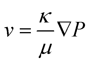
In order to use flows through a gel as a tool to manipulate concentration profiles we must understand both how to effectively control flows through gels and how concentration profiles in a gel will evolve due to diffusion.Conceptual description of flow model
First, we developed a simple model to describe the dynamics of co-flowing streams in a gel-filled microfluidic chip. Some adjustment from models based on laminar flow is required as flows through gel-filled channels have plug flow profiles6 as opposed to the typical parabolic flow profile in microchannels. Accounting for plug flow actually simplifies the typical calculations and also implies other benefits such as reduced diffusion of large molecules25 and reduced dispersion.26,27Fig. 1 schematically depicts the system, which consists of a microfluidic channel with three inlets, entirely filled with a 3D hydrogel. We wish to determine the width and lateral position of the central stream in the main channel (green in the figure) as a function of the pressures applied to the three inlets. The behavior of the streams in the main channel depends on the relative contribution of each inlet flow to the total flow in the main channel. For example, if the flow through one inlet increases, then the width of its stream in the main channel will increase while the other streams will become narrower. Therefore to model the streams in the main channel we must first determine the flow rates through each inlet channel. Since our active controls are pressures, we begin by calculating the pressure-to-flow relation of the inlet channels.
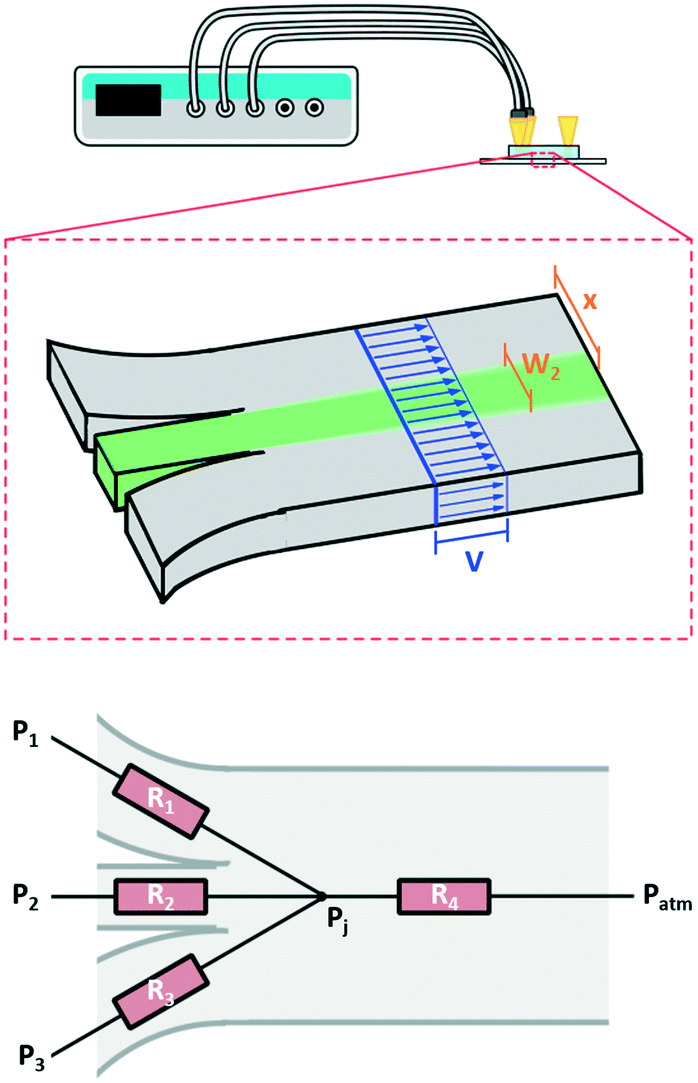 | ||
| Fig. 1 Flow in a microfluidic channel with multiple inlets connected to a pressure controller. Top, schematic of 2D device and setup showing the plug flow profile in blue, and the two geometric constraints described by eqn (5) and (6) in brown. Bottom, the resistor network used to model the system. Three inlet resistances feed into the junction and the resistance of the main channel connects the junction back to atmospheric pressure. Here our flow is through a porous media so we use the resistance as determined by Darcy's law as opposed to the typical Poiseuille resistance. | ||
Darcy flow
In order to calculate flows in terms of pressures we calculate the hydraulic resistance of the system. As stated above, all flows in our chip take place in a porous medium, so modifications to the typical flow resistance equations must be made. The textbook definition of the flow resistance for a small, non-gel-filled, channel is: | (1) |
 | (2) |
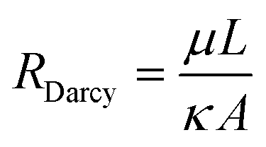 | (3) |
With the correct flow resistance for a gel in mind, we re-cast our system as the hydraulic resistor network shown in Fig. 1. In this system the flow rate in a given channel can be written in terms of the inlet pressures as:
 | (4) |
Central stream placement
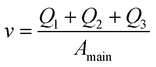
We wish to use our system to deliver solutes to certain locations in the main channel by introducing them in the central focused stream (green in Fig. 1) and changing the width and lateral position of this stream. The resistor model allows us to determine the flow rates in terms of the inlet pressures, and we will now use it to determine the inlet pressures needed at the three inlets for a specific width and lateral position of the central focused stream. To uniquely determine the three controlled pressures we develop three constraints: width, position and velocity of the central stream.For a plug flow profile in a rectangular channel, the fraction of flow that a given inlet contributes to the total flow equals the fractional width of the stream it produces with respect to the total channel width. So, for our system we can write the width of the n-th stream as:
 | (5) |
The distance between the center of the focused stream and the wall that borders stream 1 (x) can be written as:
 | (6) |
And finally we constrain the linear velocity (v) in the main channel by applying the condition:
 | (7) |
Concentration profile of diffusing compounds
We are also interested in determining how diffusion affects the concentration profiles we can create with this technique. As the streams progress through the channel, the solutes they carry will begin to diffuse causing their concentration profile to spread, thus limiting our ability to keep the concentration regions local. To calculate the 2D (where x is taken as the lateral distance and y as the downstream distance) concentration profile in the channel, we will consider it as a series of 1D concentration profiles translating down the channel at the flow velocity. If the flow rate changes, the concentration profiles require a different amount of time to move a fixed distance downstream. As diffusion has had more or less time to act, the spread of the profile at that point thus is changed when the flow rate changes.If we assume that the diffusivity of the solute does not depend on the flow rate, the textbook36 definition of the time evolution of a 1D profile that begins as a perfect plug is:
 | (8) |
If we consider the profile to be translating at a constant velocity we can rewrite eqn (8) as:
 | (9) |
We will use this equation to predict the concentration profile at a given distance downstream from the junction. Eqn (9) implies that flow velocity, diffusivity and distance from the junction are the key factors for controlling the spread of the starting profile in this technique.
Materials and methods
PDMS device fabrication
Polydimethylsiloxane (PDMS) devices were fabricated with soft lithography. Briefly, chip geometry was defined via lithography of 100 micrometers of SU8 on a silicon wafer. Inlet channels were 500 μm wide while the channel after the junction was 1.5 mm wide. PDMS (Sylgard 184) with a 10![[thin space (1/6-em)]](https://www.rsc.org/images/entities/char_2009.gif) :1 elastomer to curing agent ratio was poured over the mold and left to set for 3 hours at 60 °C. The PDMS was then removed from the mold, and 1 mm inlets were made with a biopsy punch (Harris Uni-Core). The chips were then activated in an oxygen plasma cleaner (Harrik Plasma) for 45 seconds at high power (30 Watts) and bonded to similarly treated glass microscope slides (Corning).
:1 elastomer to curing agent ratio was poured over the mold and left to set for 3 hours at 60 °C. The PDMS was then removed from the mold, and 1 mm inlets were made with a biopsy punch (Harris Uni-Core). The chips were then activated in an oxygen plasma cleaner (Harrik Plasma) for 45 seconds at high power (30 Watts) and bonded to similarly treated glass microscope slides (Corning).
For better adhesion between the PDMS and collagen, the surface of the chips were silanized with (3-aminopropyl)triethoxysilane (APTES) and treated with glutaraldehyde. To do this, the chips were first submerged in a 10% w/w APTES (Sigma-Aldrich) in water solution for 30 minutes. Devices were then briefly rinsed with 90% ethanol before being submerged in 10% w/w glutaraldehyde (Sigma-Aldrich) in phosphate-buffered saline (PBS, Sigma-Aldrich) for another 30 minutes. Finally, the chips were filled with a 4 mg mL−1 solution of titrated rat tail collagen I (Corning) and cured for 2 hours at 36 °C.
3D printed chip fabrication
The 3D version of the device was printed in Clear Resin (FormLabs) on a Formlabs Form2 3D printer. Channel dimensions were 1 × 1 mm for the inlets and 2 × 2 mm for the channel after the junction. The reader may find the STL model in the supplementary information. The surface was treated similarly to the PDMS chip for proper gel adhesion. The devices were first treated with oxygen plasma to clean the surface. Then they were submerged in a acrylamide/bis-acrylamide solution to add primary amines to the surface. The composition of coating solution used here was 9 ml 40% bis-acrylamide (BioRad), 30 ml of PBS and 22.5 μL of 10% ammonium persulfate (APS, BioRad) the chips remained submerged for 30 minutes. Then they were rinsed with 90% ethanol, treated with the glutaraldehyde solution mentioned above and filled with the titrated collagen solution mentioned above. After curing for 2 hours at 60 °C the devices were ready to use.Experimental setup
All devices shown here consist of a series of inlet channels (3 inlets for the 2D chips and 5 inlets for the 3D chips) that combine at a junction to become the single wider main channel of the device. Chip inlets were fitted with 200 μl pipette tips as reservoirs. Pressure was applied to the reservoirs via Tygon pneumatic tubing by a Fluigent pump (MFCS-EX). For the positional and width control tests in 3D and 2D chips, side inlet reservoirs were filled with PBS while the center inlet reservoir contained 0.1 mg ml−1 of 40 kDa fluorescein isothiocyanate (FITC)-labeled dextran (Sigma-Aldrich) in PBS. For the time response experiment, the side channel reservoirs still contained PBS while the center channel reservoir contained a cocktail of 0.1 mg ml−1 Alexa Fluor 647 carboxylic acid, tris(triethylammonium) (Sigma-Aldrich) and 0.1 mg ml−1 of 40 kDa FITC-labeled dextran in PBS.Experimental parameters
Positional control, width control and time response experiments were run in the 2D devices. Before a chip was used for an experimental run, a single 2 minutes calibration was done to determine the resistances of the three inlet channels and of the main channel of the chip. Details of the calibration can be found in the ESI.† From these calibrations we can also estimate a gel Darcy permeability of 4.7 × 10⁻¹⁰ cm2 which lies within the range of those found in the literature for similar gels.9 After calibration, eqn (5), (6) and (7) were used to calculate the pressures required to set: the position of the center stream, the width of the center stream, and the flow velocity. The pressures used to generate the shown concentration profiles fell in the range of 0–25 mBar depending on the device used and the desired profile. Width control was validated by setting the central stream width to 5%, 10%, 20%, 30% and 40% of the total channel width, with the stream centered in the channel and a flow velocity of 10 μm s−1. Similarly, to test positional control, the stream width was fixed at 20% of the channel width, the flow velocity was fixed at 10 μm s−1 and the distance of the center of the stream to the left wall was adjusted from 150 μm to 1350 μm in increments of 300 μm. For each tested condition, the flow was allowed to fully develop for 10 minutes before the measurement was taken and a new condition was chosen. For both experiments the resulting fluorescence profile was recorded and compared to the desired “target” profile.The target concentration profile requires some adjustment to account for diffusion in the case of the width control experiments. To do this we first measured the diffusion coefficient of the FITC dextran, as described in the supplementary information, and obtained a value of 5.5 × 10⁻¹¹ m2 s−1, a similar value to those found in the literature.24 This value was used with eqn (9) to determine the expected width of the concentration profile at 50% of maximum concentration at the measurement location. The measurement location was chosen to be 1500 μm downstream from the junction as at this point the flow had been fully developed for ∼1000 μm. We considered this the target profile width reported in Fig. 3.
In the case of the time response experiments the width and flow rate were fixed at the same values as the positional control experiment, but the target distance was instantaneously alternated from 150 μm to 1350 μm every 45 seconds. Finally, the 3D chips were run uncalibrated; the pressures needed to locate the stream in the upper right corner, the center and the lower left corner of the main channel were estimated from the 2D experiments.
All quantitative measurements of the profile were taken at 1500 μm downstream from the junction and all correlation coefficients between measured data and predicted values (R2) were calculated with MATLAB.
Results and discussion
We explored the effectiveness of our technique for controlling the position and width of co-flowing streams in a gel-filled chip. Effectiveness was evaluated by measuring the accuracy with which we could produce a desired concentration profile in the main channel of a gel-filled three-inlet device by manipulating only the inlet pressures. For a given concentration profile the model described in the theoretical section was used to determine the appropriate inlet pressures. These pressures were then applied to a device with the fluorescent dextran solution loaded in the central inlet channel and the resulting profile was compared to the desired profile.In addition, we report a brief characterization of the time response of our system and an extension of our 2D device to a fully 3D device.
Positional control of concentration profile
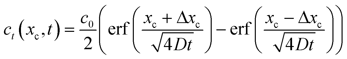
To demonstrate control of the lateral position of the central stream, we tested 5 target profiles as shown in Fig. 2. For each profile the width of the concentrated region and the total flow velocity were kept constant and only the lateral position was adjusted. We then measured the center position of the concentration profile and compared it to the target center position (Fig. 2, top).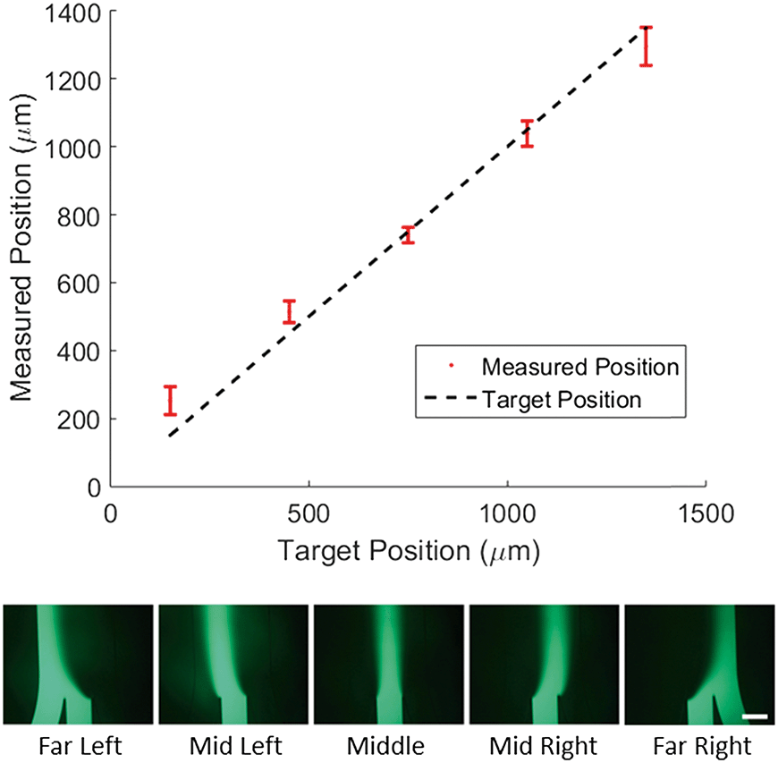 | ||
| Fig. 2 Positional control of laminar streams inside a hydrogel-filled microfluidic channel. Top, measured center position of the dye-filled stream for 5 different positions plotted against the target position. Error bars are one standard deviation, for 3 measurements each taken on a separate chip. Dotted line represents perfect agreement between target and measured position. Bottom, sample fluorescence intensity profiles from one of the chips. Note that at the far right and far left the left and right inlet channel respectively have stagnated allowing the dye to diffuse upstream, into the neighboring inlet. Scale bar is 500 μm. | ||
The direct agreement between target and measured position was strong (R2 = 0.97) with an average difference between measured and target position of 50 microns. It is worth noting that in the case of the far left and far right profiles the measured position shows a marked deviation from the target towards the center of channel. To explain this, we consider the effect of diffusion on the measurement. If the concentrated region is far from the walls of the chip, as it is for the middle profiles, diffusion spreads the profile symmetrically and the center position is unaffected. In the case of the far left and far right profiles, the concentrated region is flush with the wall of the channel, so the profile can only diffuse in the direction of the center of the channel. This asymmetric spreading shifts the center of the profile slightly towards the center of the channel as is reflected in the data.
Width control of concentration profile
To demonstrate control of the width of the focused stream, we tested 5 target concentration profiles shown in Fig. 3 (bottom). For each profile, the position of the concentrated region and the flow velocity were kept constant while only the width of the concentrated region was varied. We then plotted the measured width of the profile at 50% of maximal intensity against the target width of the profile (Fig. 3, top). The inlet pressures applied to generate the target width were specified by eqn (5) and adjusted to correct for diffusion as predicted by eqn (9). The method used for correction is outlined in the methods section.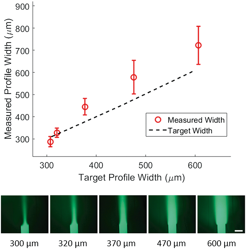 | ||
| Fig. 3 Width control of laminar streams inside a hydrogel-filled microfluidic channel. Top, width at 50% maximal intensity, measured 1.5 mm from the junction for 5 different target widths plotted against the target width for the center stream. Error bars are one standard deviation, for 3 measurements each taken on a separate chip. Linear fit is plotted over the data. Bottom, sample fluorescence intensity profiles from a single chip for a range of target stream widths from 5% of the channel width up to 40% of the channel width with the target profile widths listed below. Scale bar is 500 μm. | ||
We found a much weaker agreement between target and measurement (R2 of 0.78) than that seen for positional control, with the measured width consistently larger than the target width. Average difference between measured and target width was 62 microns. We expect that the observed difference between target and measured width can be explained by a combination of hydrodynamic effects at the junction and the diffusion in the main channel. Despite this inaccuracy, control of the width is relatively precise. This can be concluded from Fig. 3 where the deviation in measured width from device to device (error bars) is small compared to the deviation from the target width. Furthermore, measured width and target width are strongly correlated. These combined imply that the inaccuracy could be modeled and calibrated for in future work.
We include a more detailed theoretical discussion of factors affecting profile broadening in the ESI.† Summarizing this information: faster flow, a shorter main channel, or a more sharply resolved device geometry near the junction leads to less profile broadening and a steeper concentration gradient perpendicular to the flow direction. These factors can be of critical importance when adapting this technique to patterning techniques which require fine resolution with small, more diffusive molecules.
Time response of concentration profile position
When the inlet pressures of the system are changed, the change in flow profile downstream is not instantaneous. To characterize the time response we ran a series of tests where a reciprocating pattern was generated in the main channel of the device (Fig. 4). In these tests we alternated between two target profiles while keeping the flow rate and width of the concentrated region constant. Each state was held for 45 seconds before switching back to the previous state over the course of <1 second. We assumed that the delayed response of the system comes from a combination of the relaxation time of the gel,28 the compliance of the Tygon tubing used and the flow resistance of the gel-filled device. To characterize the net effect, an RC time of 61.8 seconds was calculated. | ||
| Fig. 4 Dynamic control over stream position inside a hydrogel-filled microfluidic channel. Dotted lines indicate the walls of the channel. Target profile was switched every 45 seconds and flow rate was 20 μm per second. A red (Alexa Fluor 647) and green (FITC-labeled 40 kDa dextran) dye were included in the central inlet for this test. The green channel has been subtracted from the red channel and contrast enhanced to highlight the fact that the 1 kDa red dye diffuses much faster than the 40 kDa green dye. Top, picture of both the junction and the main channel. Bottom, 5 images of the junction taken at 8.7 second intervals showing the stream shift from far left to far right orientation. Raw data is shown in Fig. SI-5.† Scale bar is 500 μm. | ||
This response time did not significantly affect our ability to generate the standing concentration profiles shown in Fig. 2 and 3. A response time of one minute is negligibly short compared to the ∼2 days (55 hours) of time needed to drain the 0.1 ml reservoirs of our device at the typical flow velocity of 10 μm s−1. For cell cultures it is furthermore not expected that time constants of less than a minute are needed. If needed, a number of measures can be taken to improve the response time of the devices. The gel-filled inlet channels were longer than necessary to facilitate interfacing and the pneumatic tubing used was flexible Tygon. For applications where a faster response time is necessary, the inlet resistance could be decreased by using shorter inlet channels and the compliance of the Tygon tubing used could be reduced by using shorter and stiffer tubing.
It is worth noting here that a simple, long-term stability experiment was also run where a static position was chosen and a 10 μm s−1 flow was maintained for 5 hours. In this test, the variation in position was 2% of the initial values. See Fig. SI-3† for further information.
Extension to 3D: controlling stream position in both horizontal and vertical direction
While a 2D junction can be used to manipulate a concentration profile in one dimension, a 3D junction can be used to manipulate a concentration profile in two dimensions. For example, consider a junction where two extra inlet channels are included that enter at the top and bottom of the center inlet channel as shown schematically in Fig. 5 top left. The central stream can still be localized horizontally as before, but with these added channels the central stream can be localized vertically as well. | ||
| Fig. 5 Top left, rendering of the 3D junction with inlets color coded. Middle left, pressures in mBar used to generate the fluorescence profiles shown in the bottom left. Bottom left, actual fluorescence intensity profiles taken from the bottom and side of the devices during experimental runs. Right, 2D position of the stream at a cross section for 3 different test conditions. Each point represents a vertical position and horizontal position measurement for a single inlet pressure configuration shown on the left. Bounds of the graph are the bounds of the main channel. Error bars are one standard deviation of the respective fluorescent profile. | ||
To show that a 3D chip with five inlets is truly capable of generating controllable concentration profiles we generated three distinct profiles and imaged them from both the bottom and side of the chip. The position and width of the resulting profiles are represented in Fig. 5 (bottom). The three distinct horizontal positions (x axis) show that the position can in fact be controlled by the pressure applied to the left and right inlets just as with the 2D device. The simultaneously plotted vertical positions (y axis) are distinct from each other and independent of the horizontal position showing that the chip allows full 3D control of the profile. The raw data and pressures used can be found in the ESI.†
Conclusion
Previously, laminar flow patterning has been used to locally deliver chemicals to flat surfaces in open microfluidic devices.1 Here we have shown that 2D and 3D laminar flow patterning through a cured hydrogel is not only possible, but relatively simple and precise to control due to the plug flow profile. Through testing of our devices we demonstrate excellent spatial control of the generated concentration profile via manipulation of the inlet pressures and are able to characterize the time response of the system. Furthermore, we show that the technique can be used in a truly 3D capacity by 3D printing and testing a version of our device with five inlets for both horizontal and vertical control of the concentration profile.Although we have only shown the ability to manipulate concentration profiles in a gel, we hope to see this technique developed as a general way to influence 3D cell cultures in a gel or 2D cell cultures on a gel/media interface. Our chips could see immediate use as a platform for locally dosing cells in 3D culture with morphogens to observe the effects of the concentration profile independently from the effects of the interstitial flowrate. Furthermore, we can generate standing gradients of morphogens perpendicular to the direction of interstitial flow, a relatively unprobed combination of stimuli. The ability to very locally dose cell cultures may also provide new techniques for guiding the development of tissues in organs-on-chips.29–31
In addition to biological applications, our technique provides a general microfluidic engineering tool to translate surface patterning techniques compatible with laminar flow patterning to a 3D matrix. For example, instead of patterning channels in 2D with soft lithography, our method would allow channels to be locally etched in a desired geometry by controlling the concentration profile of an etchant like collagenase. Also, instead of relying on 2D top down patterning techniques, our method would allow control over local stiffness of gels from the inside out by manipulating the concentration profile of a cross-linker within the gel.
In summary, our technique is a powerful extension of traditional laminar flow patterning from patterning of 2D surfaces to patterning of 3D gels. We anticipate that it will find many applications both as a general technique for patterning biological hydrogels and in particular for probing the effects of interstitial flow and morphogen gradients in 3D cell culture models and organs-on-chips.
Conflicts of interest
There are no conflicts to declare.Acknowledgements
We would like to acknowledge the European Research Council (ERC) under the Advanced Grant ‘VESCEL’ Program (Grant no. 669768) of Prof. Van den Berg for supporting this work, as well as Vasilis Papadimitriou, Mathieu Odijk, and Jorien Berendsen for thorough discussions and support during this work.References
- P. J. A. Kenis, R. F. Ismagilov and G. M. Whitesides, Science, 1999, 285, 83 CrossRef CAS PubMed.
- J. C. McDonald Takayama, E. Ostuni, M. N. Liang, P. J. A. Kenis, R. F. Ismagilov and G. M. Whitesides, Proc. Natl. Acad. Sci. U. S. A., 1999, 96, 5545 CrossRef.
- D. J. Beebe, J. Moore, J. M. Bauer, Q. Yu, R. H. Liu, C. Devadoss and B. H. Jo, Nature, 2000, 404, 588 CrossRef CAS PubMed.
- M. Shen, H. Yang, V. Sivagnanam and M. A. M. Gijs, Anal. Chem., 2010, 82, 9989 CrossRef CAS PubMed.
- S. Ramanujan, A. Pluen, T. D. McKee, E. B. Brown, Y. Boucher and R. K. Jain, Biophys. J., 2002, 83, 1650 CrossRef CAS PubMed.
- J. R. Levick, Q. J. Exp. Physiol., 1987, 72, 409 CrossRef CAS PubMed.
- D. T. Eddington and D. J. Beebe, Adv. Drug Delivery Rev., 2004, 56, 199 CrossRef CAS PubMed.
- B. Ziaie, A. Baldi, M. Lei, Y. Gu and R. A. Siegel, Adv. Drug Delivery Rev., 2004, 56, 145 CrossRef CAS PubMed.
- M. A. Swartz and M. E. Fleury, Annu. Rev. Biomed. Eng., 2007, 9, 229 CrossRef CAS PubMed.
- J. M. Rutkowski and M. A. Swartz, Trends Cell Biol., 2007, 17, 44 CrossRef CAS PubMed.
- M. A. Swartz, Adv. Drug Delivery Rev., 2001, 50, 3 CrossRef CAS.
- J. H. E. Cartwright, O. Piro and I. Tuval, Proc. Natl. Acad. Sci. U. S. A., 2003, 101, 7234 CrossRef PubMed.
- J. M. Munson and A. C. Shieh, Cancer Manage. Res, 2014, 6, 317 CrossRef PubMed.
- W. J. Polacheck, J. L. Charest and R. D. Kamm, Proc. Natl. Acad. Sci. U. S. A., 2011, 108, 11115 CrossRef CAS PubMed.
- C. P. Ng and M. A. Swartz, Am. J. Physiol., 2003, 284, 1771 Search PubMed.
- A. M. Kloxin, A. M. Kasko, C. N. Salinas and K. S. Anseth, Science, 2009, 324, 59 CrossRef CAS PubMed.
- B. M. Baker and C. S. Chen, J. Cell Sci., 2012, 125, 3015 CrossRef CAS PubMed.
- S. Trietsch, G. D. Israëls, J. Joore, T. Hankemeier and P. Vulto, Lab Chip, 2013, 13, 3548 RSC.
- B. Gumuscu, J. G. Bomer, A. van den Berg and J. C. T. Eijkel, Lab Chip, 2015, 15, 664 RSC.
- S. Chung, R. Sudo, V. Vickerman, I. K. Zervantonakis and R. D. Kamm, Ann. Biomed. Eng., 2010, 38, 1164 CrossRef PubMed.
- E. Palleau, D. Morales, M. D. Dickey and O. D. Velev, Nat. Commun., 2013, 4, 1 Search PubMed.
- C. C. Lin and K. S. Anseth, Pharm. Res., 2009, 26, 631 CrossRef CAS PubMed.
- V. S. Shirure, A. Lezia, A. Tao, L. Alonzo and S. C. George, Angiogenisis, 2017, 20, 493 CrossRef CAS PubMed.
- R. Sudo, S. Chung, I. K. Zervontonakis, V. Vikerman, Y. Toshimitsu, L. G. Griffith and R. D. Kamm, FASEB J., 2009, 23, 2155 CrossRef CAS PubMed.
- E. M. Johnson, D. A. Berk, R. K. Jain and W. M. Deen, Biophys. J., 1996, 70, 1017 CrossRef CAS.
- R. F. Ismagilov, A. D. Stroock, P. J. A. Kenis, G. Whitesides and H. A. Stone, Appl. Phys. Lett., 2000, 76, 2376 CrossRef CAS.
- A. Kamholz, B. Weigl and B. Finlayson, Anal. Chem., 1999, 71, 5340 CrossRef CAS PubMed.
- D. M. Knapp, V. H. Barocas, A. G. Moon, K. Yoo, L. R. Petzold and R. T. Tranquillo, J. Rheol., 1997, 41, 971 CrossRef CAS.
- A. D. van der Meer and A. van den Berg, Integr. Biol., 2012, 4, 461 RSC.
- S. N. Bhatia and D. E. Ingber, Nat. Biotechnol., 2014, 32, 760 CrossRef CAS PubMed.
- D. Huh, G. A. Hamilton and D. E. Ingber, Trends Cell Biol., 2011, 21, 745 CrossRef CAS PubMed.
- K. C. Boardman and M. A. Swartz, Circ. Res., 2003, 92, 801 CrossRef CAS PubMed.
- A. C. E. Helm, M. E. Fleury, A. H. Zisch, F. Boschetti, M. A. Swartz and R. Langer, Proc. Natl. Acad. Sci. U. S. A., 2017, 102, 15779 CrossRef PubMed.
- J. D. Shields, M. E. Fleury, C. Yong, A. A. Tomeri, G. J. Randolph and M. A. Swartz, Cancer Cell, 2007, 11, 526–538 CrossRef CAS PubMed.
- V. van Duinen, S. J. Trietsch, J. Joore, P. Vulto and T. Hankemeier, Curr. Opin. Biotechnol., 2015, 35, 118–126 CrossRef CAS PubMed.
- J. Crank, The mathematics of diffusion, Clarendon Press, Oxford, 1976 Search PubMed.
- S. N. Bhatia and D. E. Ingber, Nat. Biotechnol., 2014, 32, 760–772 CrossRef CAS PubMed.
- A. van der Meer and A. van den Berg, Integr. Biol., 2012, 5, 461–470 RSC.
- D. Huh, G. A. Hamilton and D. Ingber, Trends Cell Biol., 2011, 21, 745–754 CrossRef CAS PubMed.
Footnote |
| † Electronic supplementary information (ESI) available. See DOI: 10.1039/c8lc01140k |
| This journal is © The Royal Society of Chemistry 2019 |