
 Open Access Article
 This Open Access Article is licensed under a Creative Commons Attribution-Non Commercial 3.0 Unported Licence
Performance of sp-ICP-TOFMS with signal distributions fitted to a compound Poisson model
Lyndsey
Hendriks
,
Alexander
Gundlach-Graham
 * and
Detlef
Günther
* and
Detlef
Günther
Department of Chemistry and Applied Biosciences, ETH Zurich, Zurich, Switzerland. E-mail: graham@inorg.chem.ethz.ch
First published on 25th July 2019
Abstract
Accurate separation of signals from individual nanoparticles (NPs) from background ion signals is decisive to correct sizing and number-concentration determinations in single-particle (sp) ICP-MS analyses. In typical sp-ICP-MS approaches, NP signals are identified via outlier analysis based on the assumption of normally distributed (i.e. Gaussian) or Poisson-distributed background signals. However, for sp-ICP-MS with a Time-of-Flight (TOF) mass spectrometer that digitizes MS signal by fast analog-to-digital conversion (ADC), the background ion signals are neither Gaussian nor Poisson. Instead, steady-state ion signals with ICP-TOFMS follow a compound Poisson distribution that reflects noise contributions from Poisson-distributed arrival of ions and gain statistics of microchannel-plate-based ion detection. Here, we characterize this compound Poisson distribution with Monte Carlo simulations to establish net critical values (LC(ADC)) as detection decision levels for the discrimination of discrete NPs in sp-ICP-TOFMS analyses. We apply LC(ADC) to the analysis of gold-silver core–shell nanoparticles (Au–Ag NPs), and compare these results to conventional sigma-based NP-detection thresholds. Additionally, we investigate how accurate modelling of the compound Poisson TOFMS signal distribution enables separation of overlapping background and NP distributions; we demonstrate accurate size measurement of 20 nm Au NPs that have mean signal intensity of less than four counts.
1. Introduction
1.1. sp-ICP-MS and its challenges regarding the detection of increasingly smaller NPs
Coincident with a strong drive in nanotechnology to explore the promises of smaller and smaller nanoparticles (NPs)—such as 3 nm supermagnetic iron oxide NPs as positive MRI contrast agents1 or gold NPs for targeted cancer therapy2,3—continued efforts in single-particle inductively coupled plasma mass spectrometry (sp-ICP-MS) are aimed at detecting the smallest particle size. Indeed, the small size and high surface-to-volume ratio of nanoparticles compared to their ionic counterparts, strongly influence their physiochemical and toxicokinetic properties.4,5In sp-ICP-MS, accurate measurement of NP size or particle number concentration (PNC) is only possible if NP signals are distinguishable from background signals,6–8 which means that NP-size detection limits can only be improved through increasing the NP-to-dissolved background signal ratio. To accomplish this, either the instrument sensitivity can be increased or the dissolved background can be reduced. For example, dissolved background can be reduced through simple sample dilution, ion-exchange purification,9,10 NP extraction,11 or separation methods.12–14 Despite the effectiveness of the different approaches to remove dissolved analyte species, there will always be a non-zero background and, for the detection of small NPs that produce low ion-count signals, analyte sensitivity becomes the major limitation. Recall that the mass content scales with the cube of the diameter, so a 10 nm diameter Au NP, which is only 5 times smaller in diameter than a 50 nm diameter Au NP, contains little mass (∼10 ag) compared to a 50 nm Au NP (∼1260 ag). To date, the smallest detectable Au NPs are between 4–7 nm in diameter,15,16 and in order to measure NPs with half this diameter, one would require 8-times higher sensitivity. Near the size detection limit, particle signals are, by definition, similar in signal intensity to background signals, so data processing algorithms used to discriminate NP and dissolved background signals are critical. Currently, sp-ICP-MS NP identification algorithms are either based on outlier detection17–20 or deconvolution21 of the dissolved and particulate fractions.
1.2. Common approaches for finding NPs in sp-ICP-MS
The most common strategy applied in sp-ICP-MS to find NPs is to treat NP signals as outliers, and the dissolved background signals as normal objects. In this approach, a particle event is detected as an outlier if its signal intensity exceeds a defined threshold. Usually, the NP-detection threshold is determined with an iterative algorithm, which detects NPs from the dissolved background when they exceed μ + nσ, where μ is the mean of the whole dataset and nσ an integer multiple times the standard deviation.7,8,19,20 Alternatively, k-means clustering has also been discussed as an approach to separate the data into dissolved and NP fractions,22 but has not been widely used. More recently, a data evaluation approach based on Poisson statistics has been applied to determine thresholds to identify the start and end of transient signals from single NPs for data acquired with microsecond time resolution.23The basic steps of iterative outlier analysis for sp-ICP-MS are: (1) the entire dataset is averaged, (2) all events that are above μ + nσ are recognized as outliers and removed from the dataset, (3) μ and σ of the remaining dataset are recalculated and new outliers are collected, (4) iterations continue until no data are detected above the final μ + nσ threshold. Importantly, the NP-detection limit as defined here is, in fact, a decision level based solely on controlling the number of false positives (i.e. dissolved signals identified as NPs): at the NP-detection limit, by definition (assuming homoscedasticity), 50% of analyte NPs would be recorded as false negatives.24 Because we have no a priori information on shape, size, or predicted signal variance from analyte NP populations, identification of NP signals is best achieved with a decision level. In the case of μ + nσ detection decisions, in which background signal is assumed to be normally distributed (i.e. Gaussian), the μ + nσ method should find outliers (i.e. NPs) with false positive rates of 0.135%, 0.0032%, or 0.000028% (280 ppb) for n values of 3, 4, or 5, respectively. At low background ion-count rates, nσ thresholds do not accurately predict false positive rates because counting statistics dominate and the background more closely matches a Poisson distribution for pulse counting MS detectors.19
Throughout the sp-ICP-MS literature, there is no consensus on what integer value of sigma should be used to discriminate NP signals from dissolved signals. Studies independently report that 3σ,25 5σ,15,20 or even 7σ26 threshold criteria provide best NP-detection accuracy. The range of NP-detection criteria routinely used is evidence of the importance of accurate background noise characterisation. False-positive rates for NP detection thresholds above 5σ do not provide (statistically) more discrimination power for the PNCs typically measured; instead, these more restrictive NP-detection thresholds are used because the background signals cannot be fully described by a normal distribution.
1.3. Critical values as NP-detection decisions
As will be further discussed, sp-ICP-TOFMS signals measured with a fast analog-to-digital conversion (ADC) detection system are neither Gaussian nor Poisson distributed, but are best characterized as a compound Poisson distribution. This compound Poisson distribution incorporates signal variance from Poisson-distributed arrival of ions and gain statistics of microchannel-plate (MCP) based ion detection.27 Therefore, any NP-detection threshold used for sp-ICP-TOFMS should take into account the shape of the compound Poisson distribution to establish detection thresholds that have a reliable false-positive rates.In our treatment of detection criteria for sp-ICP-TOFMS, we follow the definition of detection developed by Currie28,29 and adopted by IUPAC,30 in which the minimum detectable signal (i.e. the detection decision) is termed the critical value Lc. In sp-ICP-MS, the critical value is equivalent to the NP-detection threshold: it is the signal value above which one claims all signals come from NPs.19 According to Currie, detection is, in principle, a judgement on whether an observed signal originates from the analysed sample or whether it is caused by blank or background signal. If one understands or can predict the background distribution, then one can set a critical value above which there is only a small probability that a signal comes from the background, i.e. it is a false positive. Currie defines the false positive rate as the term α. For conventional steady-state signals, an α of 0.05 (5%) is custom.29 However, in sp-ICP-MS, background events typically greatly outnumber NP events, so more conservative α values of 0.1% or even 0.01% are suggested.19,27 For example, in sp-ICP-MS measurements, often less than 10% of the dataset is occupied by NP signals. Assuming a background![[thin space (1/6-em)]](https://www.rsc.org/images/entities/char_2009.gif) :NP event ratio of 10000:1000 and NP-detection with α values of 5% and 0.1%, one would expect 500 and 10 signals falsely recognized as NP signals, respectively, which would lead to errors of +50% or +1% in particle number. Consequently, the assignment of robust NP-detection critical values in sp-ICP-MS depends both on the ability to accurately predict and describe background distributions, as well as on the selection of an appropriate α value for the expected ratio of recorded NP events to background.
:NP event ratio of 10000:1000 and NP-detection with α values of 5% and 0.1%, one would expect 500 and 10 signals falsely recognized as NP signals, respectively, which would lead to errors of +50% or +1% in particle number. Consequently, the assignment of robust NP-detection critical values in sp-ICP-MS depends both on the ability to accurately predict and describe background distributions, as well as on the selection of an appropriate α value for the expected ratio of recorded NP events to background.
In the following discussion, we demonstrate how to accurately characterize compound Poisson background distributions in sp-ICP-TOFMS and evaluate the robustness of compound-Poisson-derived net critical values (LC(ADC)), for use as NP-detection thresholds. We specifically explore the use LC(ADC) for the challenging case of detecting of small Au NPs (20 and 30 nm in diameter) that produce low-ion signals of similar magnitude to signals from the dissolved background.
2. Experimental
2.1. Materials
Dilute suspensions of commercially available monodisperse 20 nm Au NPs (18.9 ± 1.5 nm, 0.052 mg mL−1 stabilized in 2 mM citrate) and Au–Ag core–shell NPs (total diameter 61 ± 1 nm, Ag shell thickness 15 nm, Au core diameter 30 ± 3 nm, 0.021 mg mL−1 stabilized in 2 mM citrate) from NanoComposix (San Diego, CA, USA) were analyzed in this study (see Table 1 for specifications). The stock suspensions were stored in the refrigerator at 4–5 °C and allowed to warm to room temperature for 15 minutes, and then sonicated for 2 minutes prior to dilution. All dilutions were carried out in ultra-high purity (UHP) water.| Total diameter (TEM) | 61 ± 6 nm |
| Au core diameter (TEM) | 30 ± 3 nm |
| Particle concentration | 1.5 × 10¹⁰ particles per mL |
| Mass concentration (Au) | 5 μg mL−1 |
| Mass concentration (Ag) | 0.016 μg mL−1 |
| Shell thickness (calculated from total diameter) | 15.5 ± 4 nm |
| Mass Au core (calculated from Au-core diameter) | 0.28 ± 0.08 fg |
| Mass Ag shell (calculated from volume) | 1.13 ± 0.4 fg |
| Mass Ag shell (calculated from mass concentration) | 1.07 fg |
Microdroplets were used for NP mass calibration and calibration solutions were prepared by diluting commercially available single-element standard solutions of Au and Ag (Inorganic Ventures, USA) in 1% sub-boiled HNO3 and 1% HCl (VWR Chemicals, USA). 100 μg L−1 of Cs was also added to microdroplet solutions; Cs signals were used as a tracer to identify microdroplet signals. All dilutions were performed gravimetrically using a balance (Mettler AE240, Mettler-Toledo, Greifensee, Switzerland).
2.2. S(T)EM measurements
The 20 nm Au NPs were characterized by scanning (transmission) electron microscopy (S(T)EM) to assess their size distributions. Samples were prepared by pipetting a few microliters of the stock NP solution onto a glow-discharged carbon foil on copper grids. After letting the particles adsorb on the foil for 30 s, the excess NP solution was blotted off using filter paper and the samples were left to air dry. Images were recorded using an ultra-high resolution SEM (FEI Magellan 400 FEG, ThermoFisher Scientific, Eindhoven, Netherlands), operated at 30 kV in immersion lens mode. Images were simultaneously recorded with a secondary electron detector (SE) as well as by the S(T)EM detector in bright field (BF) and high angle annual dark field (HAAF) mode. Image processing was performed using the BF signal, but SE images are shown for better illustration in Fig. 6. Images were analyzed for individual particle sizes in Matlab (ver.R2017b, Mathworks Inc., MA, USA) using image processing procedures including pattern recognition and distance calibration (pixel per μm) based on the pixel size information provided in the metadata.2.3. Dual sample introduction experimental design
In this study, we used the dual sample introduction setup developed by Ramkorum-Schmidt et al.31 in combination with an ICP-TOFMS instrument (icpTOF 2R, TOFWERK AG, Switzerland), as already described elsewhere.32,33 Operating parameters for both the dual sample introduction setup and the ICP-TOFMS are provided in Table 2. Importantly, because the TOF mass analyzer provides simultaneous full mass spectrum detection at a high speed (25.136 kSpectra per s), multi-element NPs can be quantitatively measured.34–38 Online microdroplet calibration was used for NP mass quantification.32,33 In brief, NP-containing solutions were introduced through the nebulizer, while microdroplets composed of the calibration solution were produced by a microdroplet generator (50 μm diameter autodrop pipette, AD-KH-501-L6; MD-E-3000 dispensing system, Microdrop Technologies GmbH, Germany) and introduced concurrently into the ICP via a falling tube filled with a He/Ar gas mixture to accelerate droplet desolvation.39 Sensitivities recorded from microdroplets introduced concurrently with the analyte Au–Ag or Au NPs were used to calibrate mass of the NPs. In this way, online microdroplet calibration provides direct compensation for any long-term sensitivity drift. The ICP-TOFMS instrument was tuned for highest sensitivity for Ag and Au. The collision/reaction cell was pressurized with 1 mL min−1 He to promote collisional focussing and improve sensitivity.| a In order to increase the sensitivity for Au and Ag, the TOF spectral acquisition rate was adjusted from its standard value of 21.739 kHz to 25.316 kHz, which increased sensitivity of 30%, but introduced a high-m/z cut-off above 200 Th. b Averaged mass spectra are composed of data summed from 44 full mass spectra collected every 39.5 μs. Note that, for continuous liquid sample introduction of Au (see Fig. 1), the averaged spectrum acquisition rate was of 2.024 ms (i.e. 44 mass spectra at 21.739 kHz). | |
|---|---|
| Microdroplet Introduction | |
| Droplet diameter | 42.8 μm |
| Droplet frequency | 40 Hz |
| Ag concentration in droplets | 105 μg L−1 |
| Au concentration in droplets | 96 μg L−1 |
| He gas flow in falling tube | 0.56 L min−1 |
| Ar gas flow in falling tube | 0.15 L min−1 |
|
|
| Pneumatic nebulizer | |
| Nebulizer gas (Ar) | 0.82 L min−1 |
| Solution uptake rate | ∼600 μL min−1 |
|
|
| ICP conditions | |
| Intermediate gas flow (Ar) | 0.8 L min−1 |
| Outer gas flow (Ar) | 15 L min−1 |
| Power | 1550 W |
| Sampling position | 5 mm above load coil |
| Collision/reaction cell (He) | 1 mL min−1 |
|
|
| TOFMS conditions | |
| TOF spectral acquisition ratea | 25.316 kHz |
| Averaged spectrum acquisition rateb | 575.36 Hz (1.738 ms) |
2.4. Data evaluation
Averaged TOF mass spectra were recorded at a time resolution of 1.738 ms and stored in the HDF5 file format. After data acquisition, TOFMS data were processed in TOFWARE (ver. 2.5.11, TOFWERK, run in Igor-Pro 7 environment) to verify mass calibration and to export time traces of integrated mass spectral intensities of analyte isotopes and the microdroplet tracer (i.e.107Ag+, 109Ag+, 133Cs+ and 197Au+) as .csv files. Further data processing was carried out in LabVIEW (ver. 17.0.1f3, National Instruments, TX, USA).Monte Carlo simulations were used to fit ICP-TOFMS background signal distributions to a compound Poisson model in the same manner as previously described.27 Briefly, ICP-TOFMS data was truncated above the 90%-quantile (or at 3 counts, whichever is larger) in order to minimize the number of NP signals in the dataset. The background data was then iteratively modelled as a compound Poisson distribution in which the TOFMS signal acquisition is considered to be the sum of a Poisson-distributed number of ions that each sample the measured single-ion-signal (SIS) distribution of the ADC-based TOF detection system. Fitting of the background TOFMS data distribution was done with a sum of squared error (SSE) minimization procedure that globally samples a range of background count rates (λbkgd) and number of acquisitions (Nacq) to estimate values that best describe the measured data. Critical values (LC(ADC)) for NP detection were also calculated by Monte Carlo simulation with an in-house written LabVIEW program (available upon request) to approximate the relationship between LC(ADC) and λbkgd relationship for a given false-positive rate (α).27 Because LC(ADC) depends on the shape of the SIS distribution of the TOFMS detection system, we measured the SIS histogram prior to sp-ICP-TOFMS analysis. To assign a value to LC(ADC) for a given analysis, we used λbkgd determined by Monte Carlo fitting of the data and the derived expression for LC(ADC). Subtraction of Monte-Carlo simulated background from measured signal distributions was performed in LabVIEW and results were saved as frequency histograms. Processed sp-ICP-TOFMS data were plotted with OriginPro (ver 8.6.0, OriginLab Corp., MA, USA) and final figures were assembled in Adobe Illustrator (ver. 16.2.0, Adobe Systems Inc., USA).
For comparison of conventional NP-detection threshold determination methods (i.e. μ + 3σ and μ + 5σ) with our compound-Poisson-based critical value approach, iterative outlier analysis was performed in Matlab. Due to an abundance of zero-count signals in the TOFMS data, signals with zero counts were removed from the dataset prior to outlier analysis. Alternative to outlier analysis, we found that fitting signal histograms with a Gaussian function provided a better estimation of μ and σ. Gaussian fitting of the background was also performed in Matlab.
NP mass calibration was carried out using analyte sensitivities determined from the microdroplets. The signals from at least 500 microdroplets for each sp-ICP-TOFMS measurement were recorded and averaged to determine the average single-droplet signal. Microdroplets for each measurement were size-calibrated based on imaging dispensed droplets with a camera with known magnification and CMOS sensor pixel size.40 Then, as the microdroplet size and content are known, the average sensitivity in counts per unit mass of analyte in each droplet can readily be determined.41 NP diameter was calculated assuming spherical geometry of the NPs and bulk density of the NP metal.
3. Results and discussion
3.1. Compound Poisson modelling of TOFMS signals
In this work, we investigate how the description of ICP-TOFMS signals as being compound Poisson distributed affects the performance of sp-ICP-TOFMS for the detection of NPs with low-count signals. To illustrate the significance of this compound Poisson distribution, in Fig. 1 we present frequency histograms for ICP-TOFMS signals from continuous aspiration of 0.1 ng g−1 and 1 ng g−1 Au solutions collected at a time resolution of 2.024 ms. For both of these histograms, we determined the count rate (λbkgd) of the compound Poisson distribution that best describes the measured signal distributions. As seen in Fig. 1, the modelled distributions match the measured signal distributions extremely well, which is an indicator that our compound Poisson model accounts for the major sources of noise in ICP-TOFMS measurements. Furthermore, Fig. 1a shows the usual shape of low-count-rate ICP-TOFMS signal distributions, which have a high frequency zero-count bin and a right-skewed shape. Clearly, this signal distribution would not be adequately described as Gaussian or Poisson. On the other hand, in Fig. 1b it is apparent that, while a compound Poisson distribution accurately describes the data, this high-count signal could also be approximated as Gaussian,42,43 similar to high-count signals for pulse-counting MS detectors.44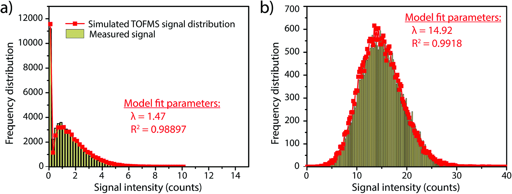 | ||
| Fig. 1 (a) Histogram of low count signals recorded from a 0.1 ng g−1 Au solution presents an unusual signal distribution shape with a large fraction of zeros and a right skewed shape; this shape can be modelled as a compound Poisson distribution that takes into account Poisson-distributed ion arrival and signal variation due to gain statistics of the TOF detection system. (b) Histogram of high-count signals recorded from a 1 ng g−1 Au solution shows an approximate Gaussian distribution because counting statistics noise dominates. In both cases, a Monte Carlo simulation that models the compound Poisson distribution of TOFMS data demonstrates an excellent match to the measured distributions. | ||
Since low-count TOFMS signals are best described with a compound Poisson distribution, the most accurate approach to establish a NP-detection threshold is to calculate net critical values specifically for this given distribution, i.e. LC(ADC). Unlike Gaussian-distributed background noise, which has well-established z-scores that allow direct calculation of LC based on measurement or estimation of σ,24,28 the compound Poisson distribution obtained with TOFMS detection does not follow a known distribution and is dependent on an empirical detector response curve, and thus cannot be simply calculated. For this reason, we estimate the relationship between LC(ADC) and λbkgd for a given false-positive rate (α) through Monte Carlo simulation of compound Poisson distributed TOF signals for a range of λbkgd values (from 0.25–25 counts per acq) and a measured SIS histogram.27 Importantly, because the compound Poisson distribution changes as a function of shape of the TOF detection system response curve (i.e. SIS histogram), routine measurements and calibration of the SIS are required to define a reliable LC(ADC). For example, SIS histograms likely vary between instruments or could change due to detector aging.
For measurements reported here, LC(ADC), is defined in eqn (1), where the α value is set conservatively to 0.0001 (0.01%).
 | (1) |
To use LC(ADC) as a detection decision to identify NPs, it is more convenient to work with the gross signal critical value (SC(ADC)), which is defined as the net critical value LC(ADC) plus λbkgd (see eqn (2)). To determine the analyte-mass detection decision (XC(ADC)), the net signal critical value (LC(ADC)) is divided by the net absolute mass sensitivity (Ai,drop) obtained from microdroplet standards, as seen in eqn (3).
 | (2) |
 | (3) |
For determination of LC(ADC) and SC(ADC), we set α = 0.01% because our analyses of Au–Ag and Au NPs have relatively few NP events compared to the background. For each sp-ICP-TOFMS analysis, we measure about 90000 data points, so α = 0.01% predicts nine false-NP signal events. Considering an acceptable false-detection rate of 10% of the total NPs, our chosen α should enable quantitative counting of NPs of down to ∼90 measured NP events. To detect lower numbers of NPs quantitatively, α would need to be lowered, which would elevate SC(ADC) and might cause non-detection of analyte NPs. In general, the choice of α for NP detection is somewhat arbitrary, and the analyst must find a useful compromise between selection of acceptable false-positive rates and NP-detection threshold.
3.2. Case study: measuring Au–Ag NPs signal distributions
To investigate the accuracy of SC(ADC) for NP identification, we measured 60 nm diameter Au–Ag core–shell NPs by sp-ICP-TOFMS and then used SC(ADC) as a NP-detection threshold to identify the Au-NP signals. Because the Ag shell contains roughly four times the mass of the Au core, the Ag signal from each NP is well above the background, and can be used as a control to record the true number of Au–Ag NPs introduced into the plasma. With this Ag control, we are able to assess the accuracy of SC(ADC) as a NP-detection criterion for the lower-count Au-NP signals, both in terms of recovery of Au–Ag NP counts and false Au-NP signals.In Fig. 2, we plot a portion of the Au–Ag NP time trace, as well as the signal-intensity frequency histograms for 107+109Ag and 197Au, respectively (see Fig. 2b and c). As displayed in Fig. 2b, the Ag NP signal distribution is baseline separated from the dissolved background signals, and a visually set threshold value of 10 counts was used to distinguish NP signals from the background. However, for 197Au+ signals, there is no clear separation between the dissolved background and NP distributions. Instead, we find a bimodal, but uninterrupted, distribution that has a very similar shape to the distribution observed in Fig. 1a. Again, most ion signals occupy the zero-count bin and a right-screwed distribution is present at slightly higher count values. To determine the fraction of the Au signal associated with the dissolved background, we fit the Au-signal distribution with our Monte Carlo method to find λbkgd and Nacq. Then, we used this λbkgd value to calculate SC(ADC). As shown in Fig. 3, thresholding Au-signals based on SC(ADC) = 2.77 counts provides accurate identification of Au-NP signals (98.3% NP recovery). The detection decision level in terms of Au-mass (XC(ADC)) is 68 ag, or ∼19 nm in diameter. We do not measure 100% of the Au NPs because some of the Au–Au NPs produce 197Au+ signals of less than 2.77 counts. Based on concomitance of found Au-NP signals and Ag-NP signals, we determined that 10 of the identified 197Au+ signals found above SC(ADC) were false positives, which is slightly less than the 26 predicted based on our assignment of α = 0.01%.
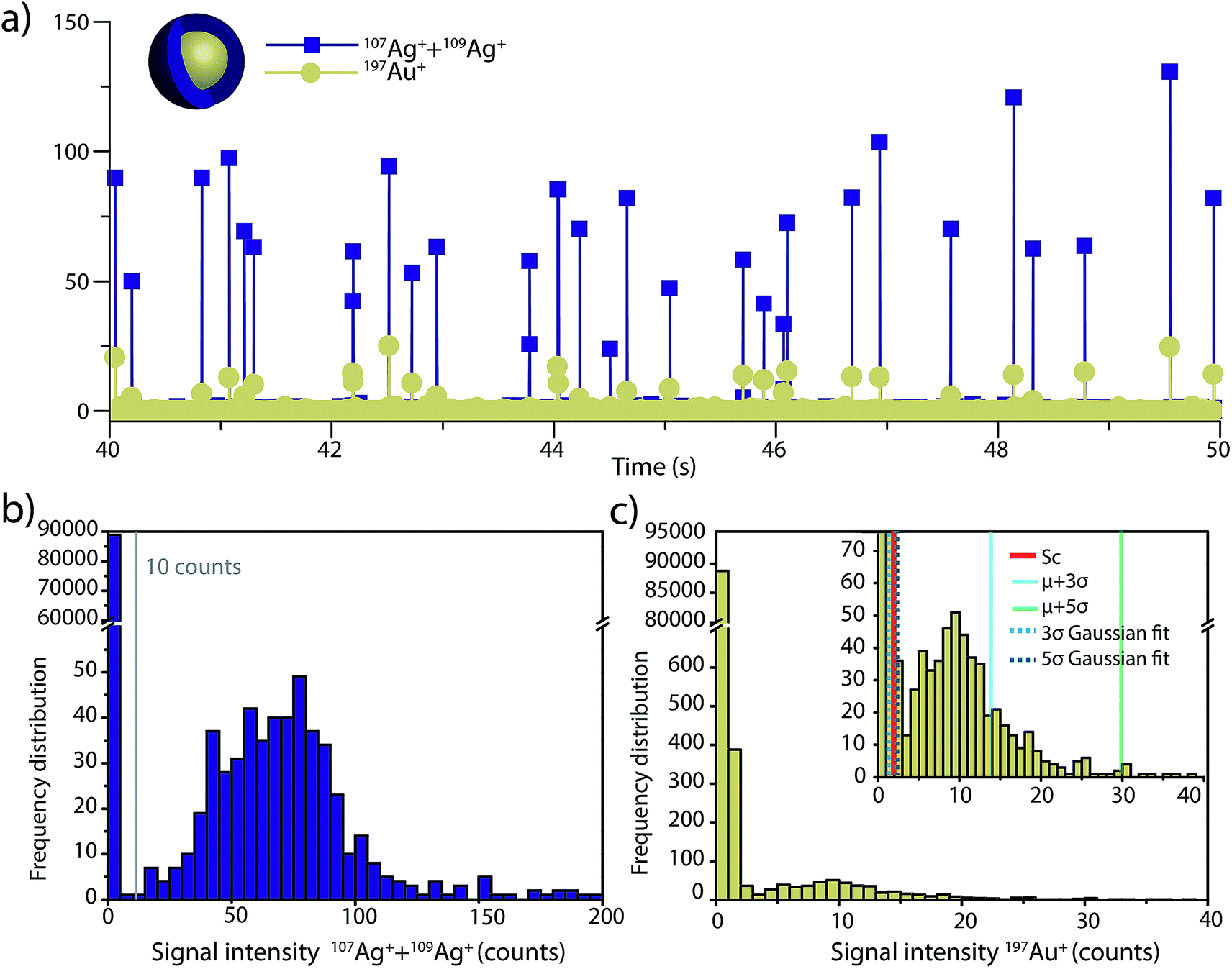 | ||
| Fig. 2 (a) sp-ICP-TOFMS time trace of the Au–Ag NPs. (b) and (c) Signal-intensity frequency distributions of the measured Au–Ag NPs for the combined signal of isotopes 107Ag and 109Ag from the shell (b) and for the 30 nm Au core (c). As the Ag signals are easily distinguished from the background, a NP detection threshold was set at 10 counts. However, for Au signals different decision threshold approaches were compared. The accuracy of the Au NPs identification can be checked by concomitance with Ag signals. | ||
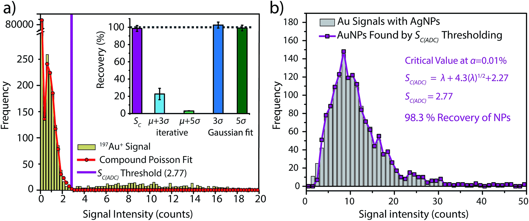 | ||
| Fig. 3 (a) Histogram of the 197Au+ signals with an overlay of the simulated background-signal distribution from our Monte Carlo approach and λbkgd = 0.012 cts per acq; the SC(ADC) NP-detection threshold is also provided. An overview of the recoveries obtained using the different NP-detection threshold approaches is presented in the inset. Error bars represent the standard deviation of three replicates. (b) Histogram of the 197Au+ signals identified above SC(ADC). True Au-NP signals are determined by 197Au+ concomitant with the control 107+109Ag+ signals. | ||
For comparison, we also attempted to identify Au-NP signals based on conventional iterative outlier analysis with outlier thresholds of μ + 3σ and μ + 5σ. In this iterative outlier analysis, we found that data with zero counts had to be removed from the dataset to prevent the threshold-value from converging to zero. However, in our particular case, when zero-count data was removed, the background:NP number ratio was low (∼2:1) and the iterative outlier analysis algorithm failed to accurately distinguish background and NP distributions, which resulted in artificially high NP-detection thresholds and low Au-NP recoveries (see Fig. 3a).
On the other hand, we also determined μ + 3σ and μ + 5σ NP-detection thresholds based on fitting the non-zero background histogram with a Gaussian function. This Gaussian-fitting procedure produced more realistic results than the iterative outlier analysis, with NP recoveries of 103% and 99% for μ + 3σ and μ + 5σ thresholds, respectively. However, it should be noted that if the non-zero-background was truly Gaussian distributed, a μ + 3σ detection threshold should produce 0.135% false positives. Consequently, as our non-zero-background is composed of ∼3000 data points, one would predict only 4 false-positive NP signals. Instead, the μ + 3σ detection decision produces 38 false-positive Au-NP signals. Deletion of zero-count data—which is the major signal level in the background—prior to background variance calculation alters the true shape of the background distribution. This signal truncation causes the calculated detection decisions to be based on fitting of incomplete datasets, and it is difficult to predict how characteristics such as background:NP event ratios or instrument response function could affect the performance of these detection decisions. The use of SC(ADC) instead of σ-based NP-detection criteria takes into account the compound Poisson nature of the ICP-TOFMS data to provide a more complete description of the dissolved background signal, and therefore offers more robust NP detection with predictable false positive rates.
In Fig. 4, we report the quantified mass of Ag and Au in each Au–Ag core–shell NP based on online microdroplet calibration, which was used to establish absolute sensitivities for 107+109Ag and 197Au.32,33 Prior to quantification, Au-NP signals were identified based on the SC(ADC) threshold. As seen, the determined element mass for both the Ag shell and the Au core matches expectations (see Table 1). For the Au core, we also plot the diameter frequency distribution—which again matches expectations. An important point to highlight here is that the use of a NP-detection threshold (i.e. SC(ADC)) enables the identification of NPs on a particle-to-particle basis. Hence, for each Au NP detected above SC(ADC), the corresponding mass of Ag in that NP can be determined, which is an important requirement for studies that classify NPs based on their multi-elemental composition.35,36,38
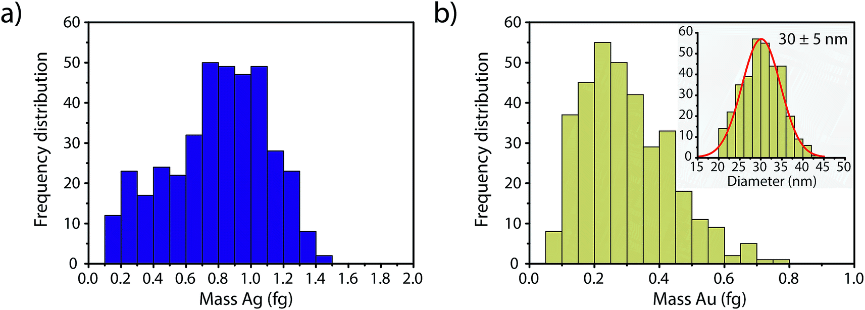 | ||
| Fig. 4 Calibrated mass frequency distributions of the Ag shell (a) and Au core (b). The Au mass frequency distribution was further converted into a size frequency distribution assuming a spherical shape and the same density as the bulk, and fitted with a normal distribution yielding a mean size of 30 ± 5 nm. | ||
3.3. Measuring single-particle distribution: application to nominal 20 nm Au NPs
In the previous section, we demonstrated that SC(ADC) is an accurate NP-detection criterion and allows for excellent NP recovery in cases where minimal overlap occurs between the dissolved background and NP signal distributions. Now, we will move on to the measurement of 20 nm Au NPs, which, based on sensitivity measured with microdroplet standards, are expected to produce ∼3.8 counts per NP. As displayed in Fig. 5, the low-count signals measured from the 20 nm Au NPs are recognizable only as a slight shoulder on the Au-signal histogram. Here again, we fit the signal distribution via our Monte Carlo approach to determine the most likely λbkgd and Nacq that describe the dissolved background distribution (see Fig. 5a). However, for this Au-signal distribution, there is no clear separation of the dissolved background and the NP distributions, so thresholding data based on SC(ADC) will result in the loss of many NP-signals that are clearly not accounted for by the compound Poisson fit. To overcome this limitation, we subtracted the Monte Carlo simulated background from the measured signal distribution. As seen in Fig. 5b, this subtraction enables recovery of NP signals with intensities lower than SC(ADC). Unfortunately, because these Au NPs are not coated with Ag as before, we cannot directly assess percent of NP recovery or false positives. Nonetheless, after calibrating 197Au+ signals to NP diameters, it becomes apparent that signals uncovered through modelled background subtraction do match well with the expected size distribution of the 20 nm Au NPs (cf.Fig. 6). While modelled background subtraction seems to allow extraction of NP signals that overlap with the dissolved background distribution, contrary to SC(ADC) NP-detection thresholding, it cannot be used to analyze particles on a particle-to-particle basis. Indeed, after modelled background subtraction, information on individual NPs is lost and only distribution-based information remains, such as size distribution or mass distribution.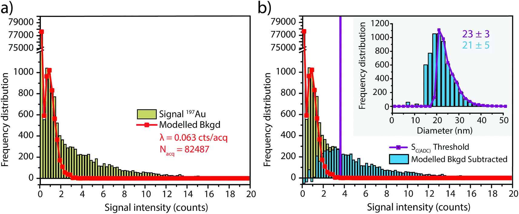 | ||
| Fig. 5 (a) Signal frequency distribution of 197Au+ signals; there is no clear separation of the signals from the 20 nm Au NPs and the dissolved background fraction. The 197Au+ signal distribution is fitted by Monte Carlo simulation to predict the dissolved background distribution. As seen, the simulated background distribution does not account for all 197Au+ signals; the remaining signals can be attributed to NPs. (b) NPs are identified using two approaches: SC(ADC) as the detection threshold and by subtraction the modelled background. The corresponding size distributions using both NP-detection approaches yield a mean sizes of 23 ± 3 nm and 21 ± 5 nm, respectively. | ||
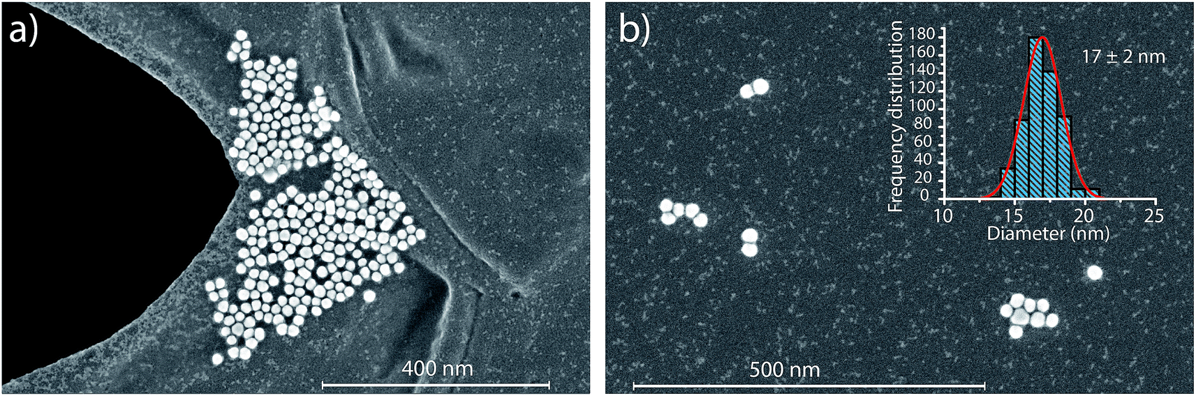 | ||
| Fig. 6 (a) S(T)EM images of the nominal 20 nm Au NPs under investigation. (b) After image analysis, 562 NPs were binned into in a size histogram and fitted with a normal distribution, yielding a mean size of 17 ± 2 nm. | ||
Sizing results are compared with S(T)EM measurements presented in Fig. 6. From the S(T)EM measurements, it can be observed that not all NPs are as spherical as initially expected. Large non-spherical particles were not accounted for in the S(T)EM data evaluation, which could explain the slightly lower average Au NP diameter found by S(T)EM image analysis compare to sp-ICP-TOFMS results.
4. Conclusion
In a previous publication, we investigated the nature of low-count TOFMS signals using microdroplets as proxy for NPs;27 here, we've applied the concept of compound Poisson background modelling through Monte Carlo simulation for the analysis of Au–Ag core–shell NPs and 20 nm Au NPs by sp-ICP-TOFMS. We demonstrated that, with sp-ICP-TOFMS, individual NPs are most accurately detected by using the critical value SC(ADC) as a detection threshold. Through the measurement of Au–Ag core–shell NPs, we showed that the decision threshold SC(ADC) yields a 98.3% NPs recovery. In contrast, the commonly applied iterative outlier analysis approach for NP detection yielded only 23% and 2% recovery, using μ + 3σ and μ + 5σ, respectively. In our example, iterative outlier analysis fails because it assumes that the background is normally distributed and that there are many more background data than NP data. There are certainly cases where iterative outlier analysis would produce reasonable NP identification with sp-ICP-TOFMS; however, the underlying assumption that background data is normally distributed is false, and this can lead to spurious results.In addition to developing NP-detection thresholds for sp-ICP-TOFMS, we also demonstrate that, in cases where NP and the dissolved fractions overlap—such as in the case of 20 nm diameter Au NPs—the subtraction of a Monte Carlo modelled distribution from the measured signal distribution can be used to predict the fraction of NPs present below SC(ADC). This treatment relies on very accurate Monte Carlo modelling of the background distribution and necessarily eliminates the information on individual particles. While modelled background subtraction is a promising approach, more work on characterizing uncertainty in Monte Carlo modelled distributions is required, especially if the approach is applied to sp-ICP-TOFMS measurement with low NP numbers.
In the presented method, the advantages of microdroplet calibration and the dual sample introduction system are combined with the new insights in TOFMS noise. Online calibration with microdroplets allows for wide flexibility in terms of materials and sizes of NPs, and also automatically compensates for plasma-related matrix effects.33 The development of more accurate noise characterization for ICP-TOFMS as demonstrated here, combined with dual sample introduction and online microdroplet calibration, make sp-ICP-TOFMS a promising method for the simultaneous quantification of diverse metal-containing NPs in terms of NP composition and number concentration in complex sample matrices.
Conflicts of interest
There are no conflicts of interest to declare.Acknowledgements
The authors thank Roland Mäder from the ETH mechanical workshop for manufacturing custom pieces necessary for the microdroplet introduction system and the dual inlet setup. L. H. acknowledges funding from Swiss National Science Foundation (SNSF) Project no. 200021 162870/1. A. G.-G. acknowledges funding through an Ambizione grant of the SNSF, project no. PZ00P2_174061. The authors acknowledge support of the Scientific Center for Optical and Electron Microscopy (ScopeM) of the Swiss Federal Institute of Technology ETHZ.References
- H. Wei, O. T. Bruns, M. G. Kaul, E. C. Hansen, M. Barch, A. Wiśniowska, O. Chen, Y. Chen, N. Li and S. Okada, Exceedingly small iron oxide nanoparticles as positive MRI contrast agents, Proc. Natl. Acad. Sci. U. S. A., 2017, 114, 2325–2330 CrossRef CAS PubMed.
- E. H. Chang, J. B. Harford, M. A. Eaton, P. M. Boisseau, A. Dube, R. Hayeshi, H. Swai and D. S. Lee, Nanomedicine: past, present and future-a global perspective, Biochem. Biophys. Res. Commun., 2015, 468, 511–517 CrossRef CAS PubMed.
- L. Zhang, F. Gu, J. Chan, A. Wang, R. Langer and O. Farokhzad, Nanoparticles in medicine: therapeutic applications and developments, Clin. Pharmacol. Ther., 2008, 83, 761–769 CrossRef CAS PubMed.
- R. D. Handy, G. Cornelis, T. Fernandes, O. Tsyusko, A. Decho, T. Sabo-Attwood, C. Metcalfe, J. A. Steevens, S. J. Klaine and A. A. Koelmans, Ecotoxicity test methods for engineered nanomaterials: practical experiences and recommendations from the bench, Environ. Toxicol. Chem., 2012, 31, 15–31 CrossRef CAS PubMed.
- O. J. Osborne, S. Lin, C. H. Chang, Z. Ji, X. Yu, X. Wang, S. Lin, T. Xia and A. E. Nel, Organ-specific and size-dependent Ag nanoparticle toxicity in gills and intestines of adult zebrafish, ACS Nano, 2015, 9, 9573–9584 CrossRef CAS PubMed.
- C. Degueldre and P. Y. Favarger, Colloid analysis by single particle inductively coupled plasma-mass spectroscopy: a feasibility study, Colloids Surf., A, 2003, 217, 137–142 CrossRef CAS.
- F. Laborda, E. Bolea and J. Jiménez-Lamana, Single Particle Inductively Coupled Plasma Mass Spectrometry: A Powerful Tool for Nanoanalysis, Anal. Chem., 2014, 86, 2270–2278 CrossRef CAS PubMed.
- H. E. Pace, N. J. Rogers, C. Jarolimek, V. A. Coleman, C. P. Higgins and J. F. Ranville, Determining Transport Efficiency for the Purpose of Counting and Sizing Nanoparticles via Single Particle Inductively Coupled Plasma Mass Spectrometry, Anal. Chem., 2011, 83, 9361–9369 CrossRef CAS PubMed.
- M. Hadioui, C. Peyrot and K. J. Wilkinson, Improvements to Single Particle ICPMS by the Online Coupling of Ion Exchange Resins, Anal. Chem., 2014, 86, 4668–4674 CrossRef CAS PubMed.
- L. Fréchette-Viens, M. Hadioui and K. J. Wilkinson, Quantification of ZnO nanoparticles and other Zn containing colloids in natural waters using a high sensitivity single particle ICP-MS, Talanta, 2019, 200, 156–162 CrossRef PubMed.
- H. El Hadri and V. A. Hackley, Investigation of cloud point extraction for the analysis of metallic nanoparticles in a soil matrix, Environ. Sci.: Nano, 2017, 4, 105–116 RSC.
- S. T. Kim, H. K. Kim, S. H. Han, E. C. Jung and S. Lee, Determination of size distribution of colloidal TiO2 nanoparticles using sedimentation field-flow fractionation combined with single particle mode of inductively coupled plasma-mass spectrometry, Microchem. J., 2013, 110, 636–642 CrossRef CAS.
- K. Proulx and K. J. Wilkinson, Separation, detection and characterisation of engineered nanoparticles in natural waters using hydrodynamic chromatography and multi-method detection (light scattering, analytical ultracentrifugation and single particle ICP-MS), Environ. Chem., 2014, 11, 392–401 CrossRef CAS.
- B. Franze, I. Strenge and C. Engelhard, Separation and detection of gold nanoparticles with capillary electrophoresis and ICP-MS in single particle mode (CE-SP-ICP-MS), J. Anal. At. Spectrom., 2017, 32, 1481–1489 RSC.
- J. Tuoriniemi, G. Cornelis and M. Hassellov, A new peak recognition algorithm for detection of ultra-small nano-particles by single particle ICP-MS using rapid time resolved data acquisition on a sector-field mass spectrometer, J. Anal. At. Spectrom., 2015, 30, 1723–1729 RSC.
- P. N. Shaw and A. Donard, Nano-particle analysis using dwell times between 10 μs and 70 μs with an upper counting limit of greater than 3 × 10⁷ cps and a gold nanoparticle detection limit of less than 10 nm diameter, J. Anal. At. Spectrom., 2016, 31, 1234–1242 RSC.
- M. S. Jiménez, M. T. Gómez, E. Bolea, F. Laborda and J. Castillo, An approach to the natural and engineered nanoparticles analysis in the environment by inductively coupled plasma mass spectrometry, Int. J. Mass Spectrom., 2011, 307, 99–104 CrossRef.
- D. M. Mitrano, A. Barber, A. Bednar, P. Westerhoff, C. P. Higgins and J. F. Ranville, Silver nanoparticle characterization using single particle ICP-MS (SP-ICP-MS) and asymmetrical flow field flow fractionation ICP-MS (AF4-ICP-MS), J. Anal. At. Spectrom., 2012, 27, 1131–1142 RSC.
- F. Laborda, J. Jimenez-Lamana, E. Bolea and J. R. Castillo, Critical considerations for the determination of nanoparticle number concentrations, size and number size distributions by single particle ICP-MS, J. Anal. At. Spectrom., 2013, 28, 1220–1232 RSC.
- J. Tuoriniemi, G. Cornelis and M. Hassellöv, Size Discrimination and Detection Capabilities of Single-Particle ICPMS for Environmental Analysis of Silver Nanoparticles, Anal. Chem., 2012, 84, 3965–3972 CrossRef CAS PubMed.
- G. Cornelis and M. Hassellov, A signal deconvolution method to discriminate smaller nanoparticles in single particle ICP-MS, J. Anal. At. Spectrom., 2014, 29, 134–144 RSC.
- X. Bi, S. Lee, J. F. Ranville, P. Sattigeri, A. Spanias, P. Herckes and P. Westerhoff, Quantitative resolution of nanoparticle sizes using single particle inductively coupled plasma mass spectrometry with the K-means clustering algorithm, J. Anal. At. Spectrom., 2014, 29, 1630–1639 RSC.
- D. Mozhayeva and C. Engelhard, A quantitative nanoparticle extraction method for microsecond time resolved single-particle ICP-MS data in the presence of a high background, J. Anal. At. Spectrom., 2019 10.1039/c9ja00042a.
- E. Voigtman, Limits of Detection in Chemical Analysis, John Wiley & Sons, Inc., USA, 2017 Search PubMed.
- C. Degueldre, P. Y. Favarger and S. Wold, Gold colloid analysis by inductively coupled plasma-mass spectrometry in a single particle mode, Anal. Chim. Acta, 2006, 555, 263–268 CrossRef CAS.
- J. Navratilova, A. Praetorius, A. Gondikas, W. Fabienke, F. von der Kammer and T. Hofmann, Detection of Engineered Copper Nanoparticles in Soil Using Single Particle ICP-MS, Int. J. Environ. Res. Public Health, 2015, 12, 15020 Search PubMed.
- A. Gundlach-Graham, L. Hendriks, K. Mehrabi and D. Günther, Monte Carlo Simulation of Low-Count Signals in Time-of-Flight Mass Spectrometry and its Application to Single-Particle Detection, Anal. Chem., 2018, 90, 11847–11855 CrossRef CAS PubMed.
- L. A. Currie, Limits for qualitative detection and quantitative determination. Application to radiochemistry, Anal. Chem., 1968, 40, 586–593 CrossRef CAS.
- L. A. Currie, in Radioactivity in the Environment, ed. P. P. Pavel, Elsevier, 2008, vol. 11, pp. 49–135 Search PubMed.
- L. A. Currie, Nomenclature in evaluation of analytical methods including detection and quantification capabilities, Pure Appl. Chem., 1995, 67, 1699–1723 CAS.
- B. Ramkorun-Schmidt, S. A. Pergantis, D. Esteban-Fernández, N. Jakubowski and D. Günther, Investigation of a Combined Microdroplet Generator and Pneumatic Nebulization System for Quantitative Determination of Metal-Containing Nanoparticles Using ICPMS, Anal. Chem., 2015, 87, 8687–8694 CrossRef CAS PubMed.
- L. Hendriks, A. Gundlach-Graham and D. Günther, Analysis of Inorganic Nanoparticles by Single-Particle Inductively Coupled Plasma Time-of-Flight Mass Spectrometry, CHIMIA International Journal for Chemistry, 2018, 72, 221–226 CrossRef CAS PubMed.
- L. Hendriks, B. Ramkorun-Schmidt, A. Gundlach-Graham, J. Koch, R. N. Grass, N. Jakubowski and D. Günther, Single-particle ICP-MS with online microdroplet calibration: toward matrix independent nanoparticle sizing, J. Anal. At. Spectrom., 2019, 34, 716–728 RSC.
- O. Borovinskaya, S. Gschwind, B. Hattendorf, M. Tanner and D. Günther, Simultaneous Mass Quantification of Nanoparticles of Different Composition in a Mixture by Microdroplet Generator-ICPTOFMS, Anal. Chem., 2014, 86, 8142–8148 CrossRef CAS PubMed.
- A. Praetorius, A. Gundlach-Graham, E. Goldberg, W. Fabienke, J. Navratilova, A. Gondikas, R. Kaegi, D. Günther, T. Hofmann and F. von der Kammer, Single-particle multi-element fingerprinting (spMEF) using inductively-coupled plasma time-of-flight mass spectrometry (ICP-TOFMS) to identify engineered nanoparticles against the elevated natural background in soils, Environ. Sci.: Nano, 2017, 4, 307–314 RSC.
- A. Gondikas, F. von der Kammer, R. Kaegi, O. Borovinskaya, E. Neubauer, J. Navratilova, A. Praetorius, G. Cornelis and T. Hofmann, Where is the nano? Analytical approaches for the detection and quantification of TiO2 engineered nanoparticles in surface waters, Environ. Sci.: Nano, 2018, 5, 313–326 RSC.
- S. Naasz, S. Weigel, O. Borovinskaya, A. Serva, C. Cascio, A. K. Undas, F. C. Simeone, H. J. P. Marvin and R. J. B. Peters, Multi-element analysis of single nanoparticles by ICP-MS using quadrupole and time-of-flight technologies, J. Anal. At. Spectrom., 2018, 33, 835–845 RSC.
- F. Loosli, J. Wang, S. Rothenberg, M. Bizimis, C. Winkler, O. Borovinskaya, L. Flamigni and M. Baalousha, Sewage spills are a major source of titanium dioxide engineered (nano)-particle release into the environment, Environ. Sci.: Nano, 2019, 6, 763–777 RSC.
- J. Koch, L. Flamigni, S. Gschwind, S. Allner, H. Longerich and D. Gunther, Accelerated evaporation of microdroplets at ambient conditions for the on-line analysis of nanoparticles by inductively-coupled plasma mass spectrometry, J. Anal. At. Spectrom., 2013, 28, 1707–1717 RSC.
- L. Flamigni, Doctor of Sciences, Doctoral Thesis, ETH Zürich, 2014 Search PubMed.
- S. Gschwind, L. Flamigni, J. Koch, O. Borovinskaya, S. Groh, K. Niemax and D. Gunther, Capabilities of inductively coupled plasma mass spectrometry for the detection of nanoparticles carried by monodisperse microdroplets, J. Anal. At. Spectrom., 2011, 26, 1166–1174 RSC.
- K. L. Hunter and R. W. Stresau, Influence of Detector Pulse Height Distribution on Abundance Accuracy in TOFMS, ETP Electron Multipliers, Australia, 1998 Search PubMed.
- A. Ipsen, Derivation from First Principles of the Statistical Distribution of the Mass Peak Intensities of MS Data, Anal. Chem., 2015, 87, 1726–1734 CrossRef CAS PubMed.
- F. Laborda, J. Medrano and J. R. Castillo, Quality of quantitative and semiquantitative results in inductively coupled plasma mass spectrometry, J. Anal. At. Spectrom., 2001, 16, 732–738 RSC.
| This journal is © The Royal Society of Chemistry 2019 |