Identification of the causes of drinking water discolouration from machine learning analysis of historical datasets

Abstract

Understanding the processes and interactions occurring within complex, ageing drinking water distribution systems is vital to ensuring the supply of safe drinking water. While many water quality samples are taken for regulatory compliance, the resulting data are often simply archived rather than being interrogated for deeper understanding due to their sparse nature across time and space and the difficulties of integrating with other data sources. This paper opens a new direction of research into distribution system water quality by mining large, historical drinking water quality datasets using machine learning techniques, in this case self-organizing maps (SOMs). Application of the methodology to national-scale datasets from three different UK water companies demonstrates the ability to identify the dominant mechanisms of iron release. Factors leading to discolouration such as low disinfectant residual, nitrification, and corrosion of unlined cast iron mains were identified at scales ranging from city to country, thereby enabling targeted interventions to ensure drinking water quality.

---

Water impact

This paper advances the management of drinking water quality in distribution systems through identification of dominant causes of discolouration. Using machine learning approaches, historical water quality databases are mined to identify site-specific relationships as well as to compare findings across scales ranging from city to region to country. The results support targeted interventions and appropriate investment to ensure water quality.

Introduction

Water utilities are tasked with managing drinking water quality across large, complex, ageing water distribution systems (WDSs) to ensure customer satisfaction and public health. As water travels from treatment works to customers through the WDS, degradation of chemical, physical and biological water quality occurs. WDS water quality is monitored to assure its quality through analysis of discrete samples for aesthetic, chemical and biological parameters, including disinfectant residual, iron, manganese, lead, turbidity, disinfection by-products, and microbial indicators.^1,2 This monitoring is sparse across time and space, with only a small percentage of locations sampled and a small volume of water collected at each. Nonetheless over the city and regional scales of WDSs, these samples cumulatively make up a large annual dataset; for example, during 2016, water companies in England tested 2 776 831 samples for water quality.³ New methodologies are needed to support transformation of this raw, sparse data into useful and actionable information for the management of networks.

There is a lack of practicable mechanistic models for prediction of WDS water quality so utilities rely on analysis of field data to prioritize interventions. But given the sparsity of data that is collected, it is difficult to understand trends and relationships among dozens of interacting variables and to create actionable information to support decisions. For large utilities operating multiple systems, such as those in the UK, prioritizing interventions is further complicated by the site-specific nature of the data collected, driving the need for globally applicable tools that can incorporate local data and identify dominant mechanisms leading to complex water quality outcomes like discolouration. Currently decisions about WDS interventions are heavily weighted to customer complaints and single noncompliant samples, leading to reactive management such as spot flushing that does not necessarily address the underlying causes of poor water quality. The advances now emerging in data analysis tools and techniques to work with incomplete and disparate data sources offers an opportunity to improve water quality understanding and support informed decision-making about interventions.

Discolouration in distribution systems

In the UK, a large number of water quality regulatory violations are related to discolouration, comprising 20% of failures in England in 2016, for example.³ Discolouration is caused by a combination of inorganic and organic compounds that, when present in the water at sufficient concentrations, result in high turbidity or colour that is noticeable by customers. Inorganic compounds of concern include metals such as iron and manganese that can originate from the source water and/or be released from the pipe wall due to corrosion reactions or hydraulic events. Due to the prevalence of iron-based pipe materials in WDSs, iron release and resulting discolouration is often simplistically related directly to the nearest iron pipes. But in reality, there are complex changes and interactions in water quality throughout the distribution system, for instance upstream unlined cast iron pipes seeding downstream plastic pipes.⁴

The characterization of discolouration in WDSs is complicated by two issues. First, primary iron corrosion is an extremely complex electro-, physico-, and bio-, chemical process. Second, while primary corrosion can contribute material for subsequent mobilization, the mechanisms of release of iron and other metals into the bulk water are often unrelated to primary corrosion and are not well understood.⁵ Factors influencing iron release and discolouration include water chemistry, microbiology, pipe material, WDS configuration, and hydraulic conditions over the entire service life of each pipe.⁶

Qualitative conceptual models for corrosion scale formation and degradation provide insight into mechanisms but have not been used for prediction of iron release at a WDS scale.⁷ Empirical models for iron release focusing on yield of colour or iron have been developed⁸ but may not be widely applicable to other systems and water chemistries.

Changes in hydraulic conditions are known to mobilize material accumulated at the pipe wall, resulting in discolouration events and non-compliance with drinking water standards.⁹ Mechanistic modelling of the hydraulic influence on water quality is hampered not only by a lack of understanding of fundamental reactions but also by uncertainty in the exact state of the network at a given time, including flow rates, pipe condition, concentration of key parameters, and degree of microbiological activity. Discolouration modelling favours empirical approaches because of this underlying complexity.⁶

Machine learning approaches in water quality

Databases maintained by water utilities include historic and updated asset records, customer contacts, discrete water quality sampling and associated laboratory analysis, and continuous/online (often hydraulic only) data collection from telemetry. The current nature of water utility data, for WDS water quality in particular, is that it remains sparse with very few locations sampled and lack of data linkages across functions. For example, water quality data is rarely linked to hydraulic model simulation results. Machine learning or data-driven analyses, which map inputs to outputs without attempting to accurately model underlying processes, can potentially yield useful understanding, such as determination of dominant variables and empirical relationships, and therefore have been used for many different environmental and water quality applications.¹⁰

To derive knowledge about the influence of variables on a numerical or categorical quantity, regression or classification techniques can be useful; these supervised techniques learn a mapping from predictor variables to output(s) given some training data. However, if the relationships between variables are poorly understood then it may be useful to apply an unsupervised clustering or dimensionality-reduction method, which typically requires little prior knowledge about the data. A simple unsupervised approach to identifying the relationships between variables in a multi-variate dataset is principle component analysis (PCA).¹¹ However, PCA cannot handle missing values in the input matrix and can only describe linear relationships between variables, making this method ill-suited to WDS water quality sampling data with its many unsampled parameters and complex reaction mechanisms.

Both the missing-values and nonlinearity limitations are overcome by the Kohonen self-organizing map (SOM),¹² a clustering and dimensionality-reduction algorithm. During the construction of a SOM, multidimensional data points are arranged in a (usually two dimensional) representation so that similar data points are clustered together. When visualized, this representation allows non-linear relationships between variables to be identified. SOMs have been used for analysis and modelling of water resources, including applications such as river flow, rainfall-runoff and surface water quality.¹³ The application of SOMs has been demonstrated in water distribution system data mining for microbiological and physico-chemical data at laboratory-scale¹⁴ as well as clustering of water quality, hydraulic modelling, and asset data for a single water supply zone.¹⁵

This paper demonstrates the application of SOMs to the complex multivariate problem of discolouration within WDS and synthesizes results from studies using country- and city-wide datasets from three UK water companies. The aim of this work is to develop and demonstrate a methodology that can overcome the current limitations of WDS water quality data to derive knowledge from historical datasets about complex processes so that utilities can make defensible decisions about maintenance and related interventions and move from a reactive to proactive maintenance strategy. Iron release and more generally discolouration were the focus of the work given the importance of these parameters in drinking water compliance in the UK.

Results and discussion

The machine learning analysis of WDS water quality data was designed and tested on large corporate databases from three large UK water companies. The databases contained multiple information sources and these varied by company depending on availability and format, including: records of physical pipe asset data, regulatory water quality sampling, and hydraulic model output. The three water companies include a diverse set of water sources, hydraulic conditions, and degree of historical problems with discolouration.

Water distribution systems studied

Water Company A serves approximately 5.4 million people via hundreds of water distribution systems with 245 water treatment works (WTW) and more than 30 000 miles of water pipes. All distribution system water quality samples from across the entire company between January 2012 and May 2016, plus the company-wide pipe asset database and WTW raw and finished water quality data were obtained and analysed for this study. A wide range of water sources, treatment processes, water chemistries, and WDS configurations are represented in this dataset.

Three cities within Water Company B were analysed in detail. WDS1, which serves a population of 142 000 people, is served by three different surface WTW using free chlorine as a secondary disinfectant with highly variable quantities of water produced at each WTW depending on localized customer demand. The resulting water quality for WDS1 is likely to be highly variable at a given location because of the daily fluctuation in source water proportions. WDS2 serves 199 000 people predominantly from a single surface water WTW (free chlorine secondary disinfectant) but with a mix of groundwater sources contributing some variability. WDS3, with a population of 261 000 people, is fully served by two nearly identical WTWs using the same surface water source (chloramine secondary disinfectant) so would be expected to have the least variability due to source water quality. WDS water quality data from the period January 2009 to December 2013 along with pipe asset data, and hydraulic model results were obtained for the study.

Water Company C serves approximately 3.1 million customers from dozens of systems with 63 WTW and more than 17 000 miles of pipe. Water quality sampling data from January 2008 to September 2014 along with pipe characteristics at the district metering area (DMA) level was compiled for the evaluation (1312 DMAs in total). Hydraulic model result and a detailed pipe asset database from GIS were not available for Company C.

Self-organising maps

The SOM training algorithm creates a mapping from a dataset to a grid of cells, where each cell has an associated reference vector. The cell shading denotes the numerical value of the reference vectors; in this study, blue denotes low and red denotes high values. The SOM output plots include the component planes for each variable as well as a U-matrix, which represents the distance and therefore dissimilarity between the reference vectors of neighbouring SOM cells. A ridge of higher values in a U-matrix plot indicates the boundary between clusters of different characteristics. Where applicable, the figures also include post analysis labelled component planes showing the relationship between categorical variables (e.g. region, pipe material) and a majority of input variables within the cell from the SOM analysis (see Fig. 1, 2 and 4).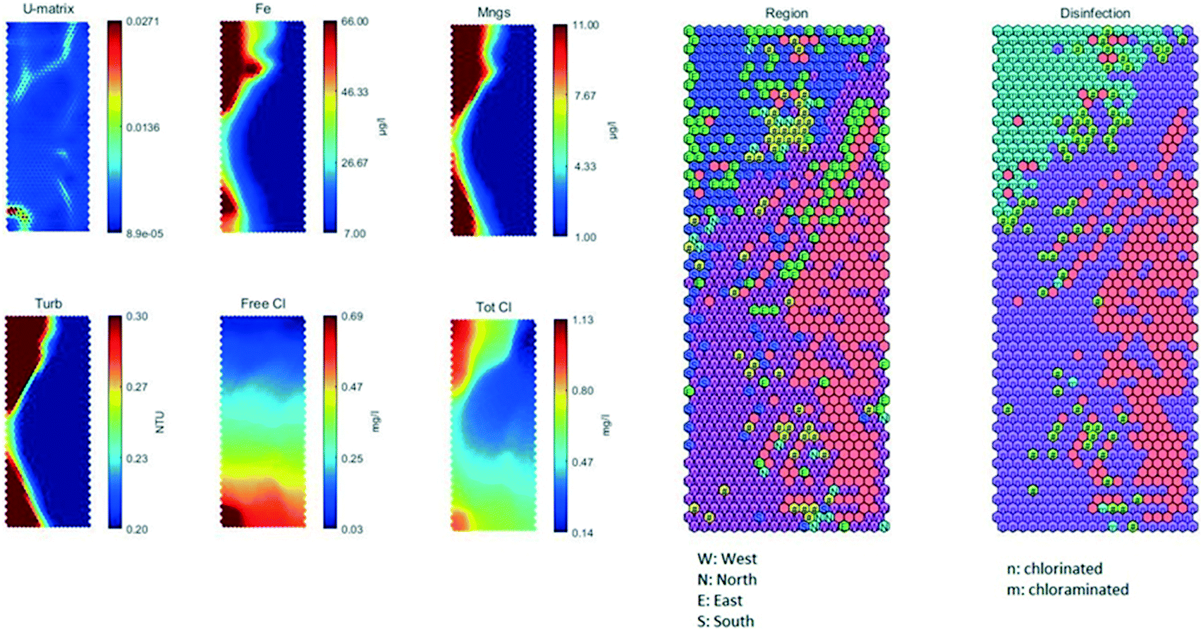

Fig. 1 SOM for Company A, labelled with region and secondary disinfectant. See Table 1 for variable definitions.

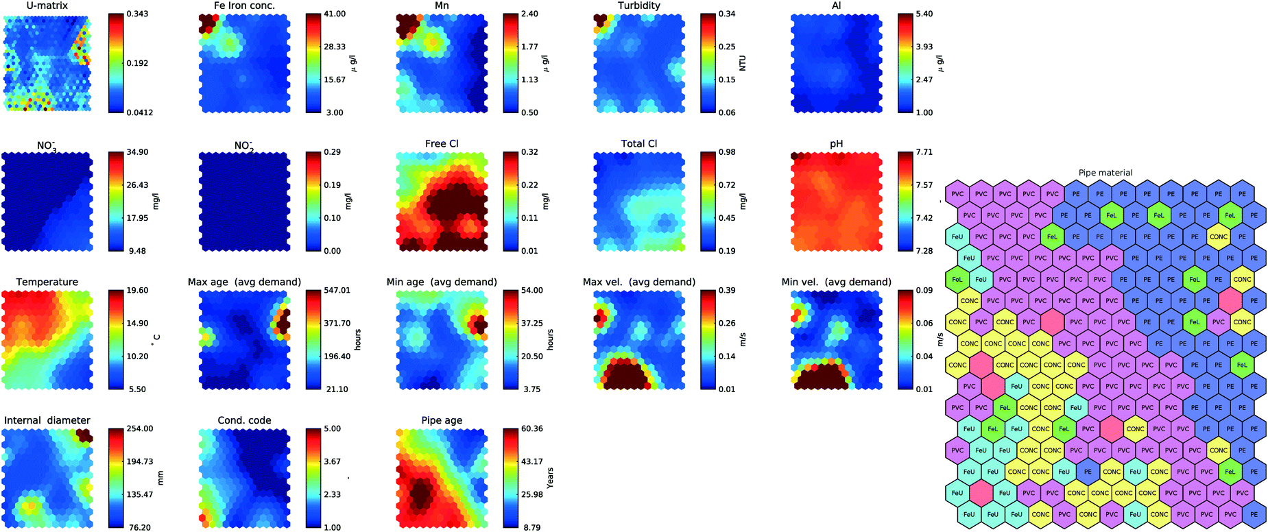Fig. 2 SOM and labelled component planes for pipe material (enlarged for visibility) for WDS1 from Company B. See Table 1 for variable definitions.

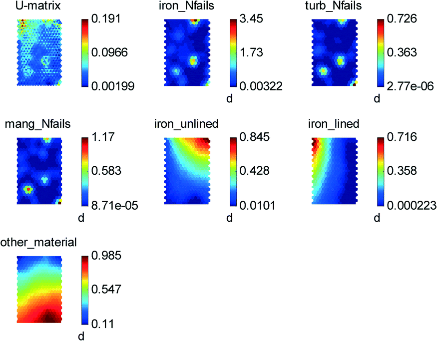Fig. 3 SOM for Company C. See Table 1 for variable definitions.

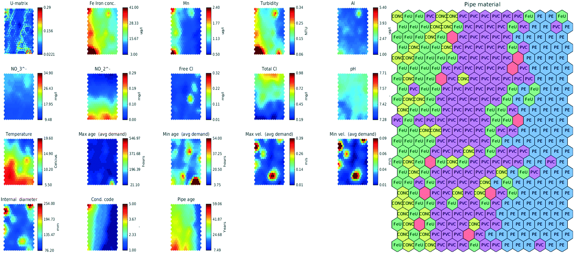Fig. 4 SOM for WDS3 in Company B, labelled with pipe material (enlarged for visibility). See Table 1 for variable definitions.

To interpret the SOMs, the plots were visually inspected to identify common patterns at the same physical location within different component and labelled planes, which indicate correlations between those variables. For example, if a red cluster for one variable occurs in the upper left corner of its component plane, a yellow cluster for a second variable in the upper left corner of that second variable's component plane can be considered to be correlated with the first variable's red cluster because it appeared at the same location. In this way, these plots can be used to identify and locate a variety of different behaviours related to discolouration as illustrated in the results to follow.

Correlation of metals with turbidity and identification of regions of interest

A SOM was produced for Company A using all regulatory samples from distribution locations (Fig. 1). This SOM was post-labelled with the region and with the type of secondary disinfection (chlorine or chloramine) to identify locations and characteristics that correlated with high iron. There are two distinct clusters visible for iron on the top left and bottom left of the component plane. These clusters correlate closely to the manganese and turbidity clusters, although the region of higher iron values in the bottom left is smaller than for turbidity and manganese. The bottom left cluster correlates to high free and total chlorine, while the top left cluster of iron correlates with high total chlorine and low free chlorine which is indicative of chloramination. This link to chloramination is confirmed in the post-training labelled component plane, in which the top left iron cluster clearly correlates to the chloraminated systems (light blue in the disinfection labelled component plane). The samples also cluster geographically, with the top left iron cluster correlating to the south region and chloramination. The bottom left iron cluster correlates to the west region (light purple in the region labelled component plane) and free chlorine systems (light purple in the disinfection labelled component plane).

In this case, the SOM showed a very strong correlation over large spatial and temporal scales (all samples nationwide, multiple years) between iron, manganese and turbidity. Given the extent of local variability amongst all of the systems across Company A, the strength of this correlation is perhaps surprising but at this scale of analysis, a few nonconforming samples will be difficult to detect. The lack of correlation between high iron and low chlorine or chloramine is also perhaps counter-intuitive. Again, small local variations are not likely visible in this SOM but the SOM does indicate that low disinfectant residual is not a predominant global factor leading to high iron and discolouration for Company A. However, conclusions about individual pipes or service areas cannot be drawn using this large scale SOM, which is better used as a screening tool to point towards further areas for analysis such as the south region chloraminated systems.

Correlation of metals with low chlorine, high temperature, and pipe material

The SOM analysis for WDS1 in Company B (Fig. 2) examined the effects of pipe material and hydraulic influences using WDS hydraulic modelling simulation results. It confirms that high iron concentrations are correlated with high manganese concentrations and high turbidity values, as indicated by the dark red area in the upper left of each component plane. The highest cluster of iron, manganese, and turbidity values also correspond to low free and total chlorine values, as well as high temperature.

There does not appear to be strong correlations between high iron and water age or velocity parameters in Fig. 2, likely because of the complicated hydraulics within WDS1 with multiple water sources and operational configurations that change the flow direction on a regular basis. Furthermore, the velocity within the pipe where the sample is collected does not fully capture the journey through the WDS that the water has taken, which may have included high velocity pipes where iron has been mobilised upstream of the sample location.

For WDS1 at Company B, there is evidence of a correlation between PVC pipe and high iron but only a small proportion of the unlined cast iron pipe appears to be correlated to elevated iron. This result indicates that a focus on cast iron pipes as the intervention to solve discolouration problems in this system may not be warranted. Furthermore, the link with high temperature and low chlorine in this case may indicate high chlorine demand and microbiological activity due to seasonal water quality changes, although this cannot be conclusively determined with the input data used in this SOM. Transport of iron from upstream WTW or unlined CI sources seem more likely than cast iron pipe deterioration as the cause of discolouration for WDS1.

For Company C, the SOM analysis was performed at the DMA level and the effect of pipe material was of particular interest. Fig. 3 shows the number of iron failures per DMA during the historical data period rather than iron concentration. This SOM has three clusters of elevated iron failures that are correlated with turbidity and manganese failures. The cluster of iron failures at the top of the component plane corresponds to DMAs with a high percentage of unlined cast iron pipe, while the other two clusters of iron failures correlate with a high percentage of other pipe material, which is predominantly plastic for Company C. Thus this example also illustrates that cast iron pipes are not necessarily the direct cause of discolouration in all DMAs.

Influence of nitrification on areas with unlined cast iron pipe

Nitrification has been associated with iron release due to microbiological activity and decreases in pH. Its occurrence can be observed when elevated nitrite and low total chlorine co-occur.¹⁶ The SOM produced for Company B, WDS3, shows some high iron concentrations in several clusters (Fig. 4). High iron is strongly correlated with high turbidity and with several clusters of high manganese (left side of planes), as well as with higher condition code which refers to older pipe with higher historical break rates.

Much of the unlined cast iron pipe (green in the pipe material labelled component plane in Fig. 4) appears to align with these high iron clusters. Some of the high iron clusters (bottom left of planes) correlate with high nitrite, low total chlorine and elevated temperature, showing the link between nitrification, unlined cast iron pipe, and high iron.

Similar results were seen for Company A in a SOM produced to explore chloraminated systems in the south region (Fig. 5). In this SOM output plot, a strong correlation between high nitrite and high iron can be seen. These clusters are linked to high turbidity. A few clusters are also correlated with high retention time in service reservoirs (middle of component planes). One cluster of slightly elevated iron appears to be correlated with higher WTW organic carbon and higher WTW turbidity (lower right of component planes). The iron clusters correlate with high percentage of cast iron or spun iron pipe in most cases with the exception of the moderate iron cluster at the bottom of the component plane, which is more strongly correlated with high percentage of ductile iron pipe.

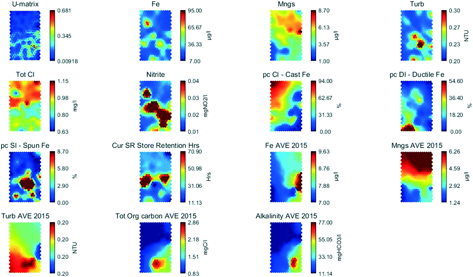Fig. 5 SOM for south region, chloraminated systems in Company A. See Table 1 for variable definitions.

The strong relationship between nitrification indicators and high iron for certain unlined cast iron pipes in Fig. 4 and 5 demonstrate the impact of this phenomenon at two different scales (regional and city). This finding agrees with previous studies that have shown scale destabilization to occur when there are low oxidant concentrations,⁸ an increase in microbiological activity, and nitrification.¹⁶ However, not all of the nitrification is associated with increased metals or turbidity. These findings emphasize the need for good nitrification management as a discolouration intervention, including total organic carbon reduction in the treated water, residual disinfectant management and active control of water circulation.

Experimental

Data extraction and processing

For each water company dataset, raw data was collated, cleaned, links between separate databases were created by spatial analysis or pipe identification number, and summary variables were calculated (Table 1). Spatial connectivity was also determined such that individual pipes serving sampling locations or DMAs could be matched to their corresponding WTW and service reservoirs (SRs). Considerable effort was required to assemble the datasets for each company, particularly to match water quality sample tap collection locations to the correct pipe, to verify connectivity, to fill in missing values in pipe asset data such as diameter and material to the extent possible, and to match hydraulic model results to the pipe from which each water quality sample was collected (Company B only). Minimal outlier removal was performed during the data pre-processing stage. The values of water quality samples with undetectable concentrations were set to half the limit of detection for the relevant parameter.

Table 1 Summary of variables and data sources used in analysis

Variable (units)	Short form variable name	Data source	Included in SOM analysis by Company			Comments
			A	B	C
Iron (mg L^−1)	Fe iron conc., Fe	Water quality	Y	Y	Y	Routine WDS measurements plus additional samples to investigate events
Manganese (mg L^−1)	Mn, Mngs	Water quality	Y	Y	Y	Routine WDS measurements plus additional samples to investigate events
Turbidity (NTU)	Turbidity, Turb	Water quality	Y	Y	Y	Routine WDS measurements plus additionalsamples to investigate events
Aluminium (μg L^−1)	Al	Water quality	N	Y	N	Routine WDS measurements plus additional samples to investigate events
Nitrate (mg L^−1)	NO3^−	Water quality	N	Y	N	Routine WDS measurements plus additional samples to investigate events
Nitrite (mg L^−1)	NO2^−, nitrite	Water quality	Y	Y	N	Routine WDS measurements plus additional samples to investigate events, chloraminated systems only
Free chlorine (mg L^−1)	Free Cl	Water quality	Y	Y	Y	Routine WDS measurements plus additional samples to investigate events
Total chlorine (mg L^−1)	Total Cl, Tot Cl	Water quality	Y	Y	Y	Routine WDS measurements plus additional samples to investigate events
pH	pH	Water quality	N	Y	Y	Routine WDS measurements plus additional samples to investigate events
Temperature (°C)	Temperature	Water quality	N	Y	Y	Routine WDS measurements plus additional samples to investigate events
Iron failures	Iron_Nfails	Calculated	N	N	Y	Calculated number of regulatory failures by DMA
Manganese failures	Mang_Nfails	Calculated	N	N	Y	Calculated number of regulatory failures by DMA
Turbidity failures	Turb_Nfails	Calculated	N	N	Y	Calculated number of regulatory failures by DMA
Average WTW iron (mg L^−1)	Fe AVE	Water quality	Y	N	N	Annual average in finished water at WTW
Average WTW manganese (mg L^−1)	Mngs AVE	Water quality	Y	N	N	Annual average in finished water at WTW
Average WTW total organic carbon (mg L^−1)	Tot org carbon AVE	Water quality	Y	N	N	Annual average in finished water at WTW
Pipe internal diameter (mm)	Internal diameter	Asset database	Y	Y	N	Nominal value used for Company A, actual value used for Company B
Condition code	Cond. code	Asset database	N	Y	N	Derived from asset management system based on maintenance history, inspection data, and other related information, values from 1 (good condition) to 5 (poor condition)
Pipe material	Pipe material	Asset database	N	Y	N	Categorised into 8 groupings of similar material for Company B: iron unlined (FeU), iron lined (FeL), polyvinyl chloride (PVC), polyethylene (PE), steel (ST), concrete (CONC), lead (PB), and unknown (?)
Percentage of cast iron pipe in DMA	Pc CI – cast Fe, iron_unlined	Asset database	Y	N	Y	Pipe asset data, considered to be unlined pipe
Percentage of ductile iron pipe in DMA	Pc DI – ductile Fe, iron_lined	Asset database	Y	N	Y	Pipe asset data, considered to be lined pipe
Percentage of spun iron pipe in DMA	Pc SI – spun Fe	Asset database	Y	N	N	Pipe asset data, considered to be unlined pipe; not differentiated from cast iron for Company C
Percentage of non-metallic pipe in DMA	Other_material	Asset database	N	N	Y	Pipe asset data
Minimum velocity (m s^−1)	Min vel. (avg demand)	Hydraulic model	N	Y	N	Samples linked to pipes by asset ID, maximum value over average hydraulic simulation with 24-hour demand patterns
Maximum velocity (m s^−1)	Max vel. (avg demand)	Hydraulic model	N	Y	N	Samples linked to pipes by asset ID, maximum value over average hydraulic simulation with 24-hour demand patterns
Minimum water age (h)	Min age (avg demand)	Hydraulic model	N	Y	N	Samples linked to pipes by asset ID, maximum value over average hydraulic simulation with 24-hour demand patterns
Maximum water age (h)	Max age (avg demand)	Hydraulic model	N	Y	N	Samples linked to pipes by asset ID, maximum value over average hydraulic simulation with 24-hour demand patterns
Service reservoir retention (h)	Cur SR store retention h	Standalone data	Y	N	N	Company A, internal calculations of retention time within reservoirs (tanks)
Pipe age	Pipe age	Calculated	N	Y	N	Based on pipe installation date

---

SOM analysis

An issue requiring attention when using SOMs is the selection of significant input variables. The inclusion of too many variables can increase computational complexity, create difficulty in learning, and result in misconvergence.¹³ Conversely, inclusion of too few variables can miss important trends or relationships. The spatial scale of data inclusion is also important and was explored extensively for Company A. Multiple preliminary analyses were performed to determine the list of variables to include in the analysis (Table 1). Water quality sampling data for infrequently measured parameters such as disinfection by-products were excluded for sparsity and lack of connection to discolouration outcomes but could be used for other water quality evaluations. While customer complaint data was also available, it was not included in the analysis due to the inherent variability and subjective nature of individual customer behaviour.

When plotting component planes, the SOM Toolbox by default sets each colour bar scale to the numerical range of the corresponding dimension of the set of reference vectors. Under these conditions, the SOM for the analysis of each individual WDS would have a different value assigned to each colour to reflect the range in values within the given dataset only, making it difficult to compare results from different study areas. Additionally, outliers within the input data can skew the colour shading within the SOM component planes, with a resulting loss of detail for the values closer to the median. To ensure that the analysis produced consistent results over all study areas, the mapping from numerical input data ranges to colour bar ranges was standardized using the 5th (low value, blue colour) and 95th (high value, red colour) percentile for the combined dataset across all study areas (‘reference ranges’). Outliers beyond those values were not required to be removed from the datasets but rather would be shown as the high or low value colour. Retention of outliers in the analysis of water quality is desirable in that they may characterize atypical water quality events that are of interest. The size and number of hexagons making up the component plane is a function of the size of the input dataset and the strength of the clustering relationships so the output plots look slightly different across the analyses.

The SOMs presented in this study were generated using the Imputation SOM algorithm¹⁷ as implemented in the SOM Toolbox v2.1 for MATLAB,¹⁸ which provides a robust handling of missing values in the training dataset compared to the standard algorithms.

Conclusions

Self-organising maps have been shown to be powerful for analysis of WDS water quality trends and relationships, in particular overcoming the challenges associated with sparse data and spatial scales ranging from DMA to region to country. The SOM was able to capture the strong correlation over large spatial and temporal scales (for example all samples nationwide, multiple years as in Fig. 1) between iron, manganese and turbidity. While it is possible to determine the region with highest iron concentrations without advanced machine-learning techniques, the SOM output plot offers a simple and straightforward way to demonstrate the strength of trends and multivariate correlations, especially for non-technical stakeholders, and thus has value as a visualization technique as well as an analytical one. The national-scale SOM can provide an important initial screening of the full dataset to guide further investigation, thereby demonstrating the need to tailor the extent of input data to the question(s) under consideration. The effort required to clean and compile a national WDS water quality dataset can be considerable but once created, further analyses, such as the one shown in Fig. 5 for Company A, can be quickly completed through simple queries to isolate subsets of the data.

Cast iron pipes are often the focus of a discolouration analysis and, as with most UK water companies and many internationally, the companies in this study have extensive quantities of unlined cast iron and similar pipes in service. This study demonstrates that not all unlined cast iron pipes were associated with high iron, meaning that some pipes are performing well despite their age and/or condition. Understanding that the dominant mechanism of discolouration risk is not necessarily the deterioration of the cast iron pipes themselves allows for appropriate interventions to be selected and could avoid unnecessary rehabilitation or replacement of cast iron pipe. For Company C, the ability to identify a few high-risk DMAs where high iron is associated with unlined cast iron pipe has successfully directed their intervention strategies.^19,20

There are many different mechanisms that can result in iron release and discolouration in a WDS but not all will occur to the same extent in every system over space and time so identifying the dominant mechanism(s) is a key research and WDS management need. In this study, the data-driven analysis techniques provide insight into the dominant mechanisms influencing iron release and discolouration for each of the systems. The method has proven to be particularly robust yet flexible, given that each water company had different types of data available for the analysis and considered different questions related to discolouration over different spatial scales and time periods. The method has captured system-specific factors and has facilitated comparisons between systems and regions by using different sets of input variables selected at different groupings and scales.

Interpretation of the SOM output plots is manual and subjective so this method is not suited to all types of historical data mining analyses. However, within this study the interpretation task was found to be a valuable opportunity for operational staff to derive a deeper understanding of system performance and allowed for their expert knowledge to be incorporated. Most importantly, the concept of extracting value and knowledge from historical water quality data, which has taken considerable effort and expense to collect but is frequently archived and forgotten, needs to be embraced across the water sector so further data mining research in this field should be pursued.

Conflicts of interest

There are no conflicts to declare.

Acknowledgements

The authors gratefully acknowledge the contributions and financial support of a number of individuals who assisted with the multiple studies described herein, including Jonathan Edwards, Will Furnass, Kate Ellis, Gavin Sailor, and Ehsan Kazemi at the University of Sheffield; Barrie Holden, Paul Crawley and Robin Price at Anglian Water; Natalie Jakomis at Dwr Cymru Welsh Water; Leon Nam and Ross O'Rourke at RPS Group; David Main, Bill Reekie, and Mira Hanova at Scottish Water. This work was also supported by the UK EPSRC under grants EP/N010124/1, EP/I029346/1 and EP/G029946/1.

Notes and references

1. Drinking Water Inspectorate (DWI). The Water Supply Regulations 2010, Statutory Instruments 2010 No. 991.
2. United States Environmental Protection Agency (USEPA), National primary drinking water regulations, CFR Title 40, vol. 22, Part 141, 2010.
3. DWI. Drinking water 2016, summary of the Chief Inspector's report for drinking water in England, http://dwi.defra.gov.uk/about/annual-report/2016/Drinking_water_2016_Public%20_water_supplies_England.pdf, 2017.
4. P. S. Husband and J. B. Boxall, Asset deterioration and discolouration in water distribution systems, Water Res., 2011, 45(1), 113–124.
5. A. S. Benson, A. M. Dietrich and D. L. Gallagher, Evaluation of iron release models for water distribution systems, Crit. Rev. Environ. Sci. Technol., 2012, 42(1), 44–97.
6. J. Vreeburg and J. Boxall, Discolouration in potable water distribution systems: A review, Water Res., 2007, 41(3), 519–529.
7. P. Sarin, V. L. Snoeyink, D. A. Lytle and W. M. Kriven, Iron corrosion scales: Model for scale growth, iron release, and colored water formation, J. Environ. Eng., 2004, 130(4), 364–373.
8. S. A. Imran, J. D. Dietz, G. Mutoti, J. S. Taylor and A. A. Randall, Red water release in drinking water distribution systems, J. - Am. Water Works Assoc., 2005, 97(9), 93–100.
9. J. B. Boxall and A. J. Saul, Modelling discolouration in potable water distribution systems, J. Environ. Eng., 2005, 131(5), 716–725.
10. D. P. Solomatine and A. Ostfeld, Data-driven modelling: some past experiences and new approaches, J. Hydroinf., 2008, 10(3), 3–22.
11. E. Oja, Subspace Methods of Pattern Recognition, Research Studies Press, Letchworth, England, 1983.
12. T. Kohonen, The self-organizing map, Proc. IEEE, 1990, 78(9), 1464–1480.
13. A. M. Kalteh, P. Hjorth and R. Berndtsson, Review of the self-organizing map (SOM) approach in water resources: Analysis, modelling and application, Environ. Model. Softw., 2008, 23(7), 835–845.
14. S. R. Mounce, I. Douterelo, R. Sharpe and J. B. Boxall, A bio-hydroinformatics application of self-organizing map neural networks for assessing microbial and physico-chemical water quality in distribution systems, Proceedings of 10th International Conference on Hydroinformatics, Hamburg, Germany, 2012.
15. S. R. Mounce, R. Sharpe, V. Speight, B. Holden and J. B. Boxall, Knowledge discovery from large disparate corporate databases using self-organising maps to help ensure supply of high quality potable water, Proceedings of 11th International Conference on Hydroinformatics, New York, USA, 2014.
16. American Water Works Association (AWWA). Nitrification in Chloraminated Distribution Systems: Fundamentals, Prevention and Control, Manual of Water Supply Practice M56, Denver, CO, 2003.
17. Advances in Self-Organizing Maps subtitle of the Special Issue: Selected Papers from the Workshop on Self-Organizing Maps 2012 T. Vatanen, M. Osmala, T. Raiko, K. Lagus, M. Sysi-Aho, M. Orešič, T. Honkela and H. Lähdesmäki, Self-organization and missing values in SOM and GTM, Neurocomputing, 2015, 147, 60–70.
18. Helsinki University of Technology. SOM Toolbox (for MATLAB), Github repository, https://github.com/ilarinieminen/SOM-Toolbox/git commit ID: bc7fa9bc6e6f738577d02f34c8ffbae4bbf4d1c1, based on v2.1, 2015.
19. K. Ellis, S. R. Mounce, J. Edwards, V. Speight, N. Jakomis and J. Boxall, Interpreting and estimating the risk of iron failures, Procedia Eng., 2015, 119, 299–308.
20. S. R. Mounce, K. Ellis, J. M. Edwards, V. L. Speight, N. Jakomis and J. B. Boxall, Ensemble decision tree models using RUSBoost for estimating risk of iron failure in drinking water distribution systems, Water Resources Management, 2017, 31, 1575–1589.

---