
 Open Access Article
 This Open Access Article is licensed under a
 Creative Commons Attribution 3.0 Unported Licence
Powering sustainable development within planetary boundaries†
Ibrahim M.
Algunaibet
 a,
Carlos
Pozo
a,
Ángel
Galán-Martín
a,
Mark A. J.
Huijbregts
b,
Niall
Mac Dowell
ac and
Gonzalo
Guillén-Gosálbez
*ad
a,
Carlos
Pozo
a,
Ángel
Galán-Martín
a,
Mark A. J.
Huijbregts
b,
Niall
Mac Dowell
ac and
Gonzalo
Guillén-Gosálbez
*ad
aCentre for Process Systems Engineering, Department of Chemical Engineering, Imperial College London, South Kensington Campus, London SW7 2AZ, UK
bDepartment of Environmental Science, Institute for Water and Wetland Research, Radboud University, P.O. Box 9010, NL-6500, GL, Nijmegen, The Netherlands
cCentre for Environmental Policy, Imperial College London, South Kensington Campus, London SW7 1NA, UK
dInstitute for Chemical and Bioengineering, Department of Chemistry and Applied Biosciences, ETH Zürich, Vladimir-Prelog-Weg 1, 8093 Zürich, Switzerland. E-mail: gonzalo.guillen.gosalbez1@chem.ethz.ch
First published on 24th January 2019
Abstract
The concept of planetary boundaries identifies a safe space for humanity. Current energy systems are primarily designed with a focus on total cost minimization and bounds on greenhouse gas emissions. Omitting planetary boundaries in energy systems design can lead to energy mixes unable to power our sustainable development. To overcome this conceptual limitation, we here incorporate planetary boundaries into energy systems models, explicitly linking energy generation with the Earth's ecological limits. Taking the United States as a testbed, we found that the least cost energy mix that would meet the Paris Agreement 2 degrees Celsius target still transgresses five out of eight planetary boundaries. It is possible to meet seven out of eight planetary boundaries concurrently by incurring a doubling of the cost compared to the least cost energy mix solution (1.3% of the United States gross domestic product in 2017). Due to the stringent downscaled planetary boundary on biogeochemical nitrogen flow, there is no energy mix in the United States capable of satisfying all planetary boundaries concurrently. Our work highlights the importance of considering planetary boundaries in energy systems design and paves the way for further research on how to effectively accomplish such integration in energy related studies.
Broader contextPlanetary boundaries are global limits on environmental flows that should never be transgressed to prevent the occurrence of catastrophic nonlinear events challenging the Earth's ecological capacity. Motivated by the planetary boundaries concept, the World Business Council for Sustainable Development created a clear sustainable pathway known as Action2020, which reflects upon the global momentum towards a broader scope of environmental policies going beyond greenhouse gas emissions. The power sector is key to sustainability, yet it has never been studied through the lens of planetary boundaries. Energy systems are intrinsically complex due to the wide range of engineering and reliability constraints governing their behavior. Developing decision-support tools for designing energy systems meeting these constraints while operating within planetary boundaries is considered critical. Here, we provide an approach that (i) characterizes environmental flows of electricity technologies in terms of planetary boundaries contributions, (ii) downscales planetary boundaries to the regional and sectoral level and (iii) incorporates both pieces of information into energy systems models to design more sustainable energy mixes. Our approach can assist in designing energy mixes that meet planetary boundaries, while opening up new avenues for the widespread incorporation of planetary boundaries in energy related problems. |
Introduction
Designing sustainable energy mixes of the future is a complex task that requires the use of energy systems models (ESMs) to support decision-making. ESMs available at present identify electricity mixes that minimize the total cost while meeting a set of technical constraints, including demand satisfaction and capacity limitations. MARKAL/TIMES,1 NEMS,2 SWITCH3,4 and Electricity Systems Optimization (ESO)5 are examples of ESMs that follow the same mathematical principles and general approach while differing in the modeling assumptions and data sources.In past years, it has become clear that reducing Greenhouse Gas (GHG) emissions6–10 is not sufficient to ensure our sustainable development, since other key environmental impacts cannot be overlooked (e.g., land-system changes or freshwater use). Hence, ESMs face at present the challenge of embracing additional environmental criteria beyond cost minimization to guide us towards sustainable energy systems. Recent works incorporated environmental impacts in ESMs following primarily Life Cycle Assessment (LCA) principles.11–14 Unfortunately, while enabling a deeper environmental analysis, the integration of LCA with ESMs fails to provide absolute bounds on the impact of an energy mix and, consequently, cannot identify sustainable energy mixes guaranteed to operate within the Earth's ecological capacity.15 Here, we present an approach to assist in the design of sustainable energy mixes based on the concept of Planetary Boundaries (PBs),16 a set of ecological limits that should never be transgressed by our planet to operate safely. Originally introduced by Rockström et al.,17 PBs on nine out of ten Earth-system Processes (ESPs) identify thresholds for humanity that, if surpassed, may trigger a series of nonlinear changes with unpredictable effects at a global scale.18 By including PBs in ESMs, we here link unambiguously the performance of electricity generation technologies with their wide environmental impact, ultimately designing energy mixes fully consistent with the Sustainable Development Goals.19,20
To demonstrate the capabilities of our approach, the United States (US) was taken as a testbed to discuss the implications of including PBs in energy systems design. Our previously developed ESM for the US, the Emissions Reduction Cooperation Model (ERCOM),6 was modified to include planetary boundaries (ERCOM with Planetary Boundaries (ERCOM-PB) henceforth) to ultimately identify mixes operating below all PBs and to analyze the economic implications thereof. We found that the Business as Usual (BAU) energy mix, i.e., the US 2012 default developments in the power sector required to meet the 2030 electricity demand, transgresses six out of the eight PBs considered, including the climate change PBs. Furthermore, the least cost energy mix, which is in line with the 2 degrees Celsius (°C) target governed by the Paris Agreement (the Paris Agreement solution henceforth), transgresses five out of the eight PBs, including those on climate change, though in this solution the magnitude of the transgression is lower. Our model could not identify any single mix satisfying all the shares of PBs assigned to the US power sector concurrently, yet seven of the eight PBs could be met simultaneously with an energy mix relying on wind (both onshore and offshore), natural gas with Carbon Capture and Storage (CCS), hydropower and Bio-energy with CCS (BECCS). This mix would incur an extra cost of 40% compared to the BAU solution (or 0.8% of the US Gross Domestic Product (GDP) in 2017), while doubling the cost of the Paris Agreement solution (or an extra cost equal to 1.3% of the US GDP in 2017). This extra cost needed to improve the performance of the mix in terms of PBs would be associated with mandatory investments in relatively expensive electricity technologies, such as wind offshore, natural gas with CCS and BECCS.
Modeling framework
When attempting to incorporate PBs into ESMs, two main challenges were addressed (Fig. 1): (i) downscaling PBs, originally defined for the Earth as a whole, to the country and sectoral level; and (ii) linking the operation of energy technologies to their performance in terms of PBs via the environmental flows they generate. We discuss both challenges in detail next.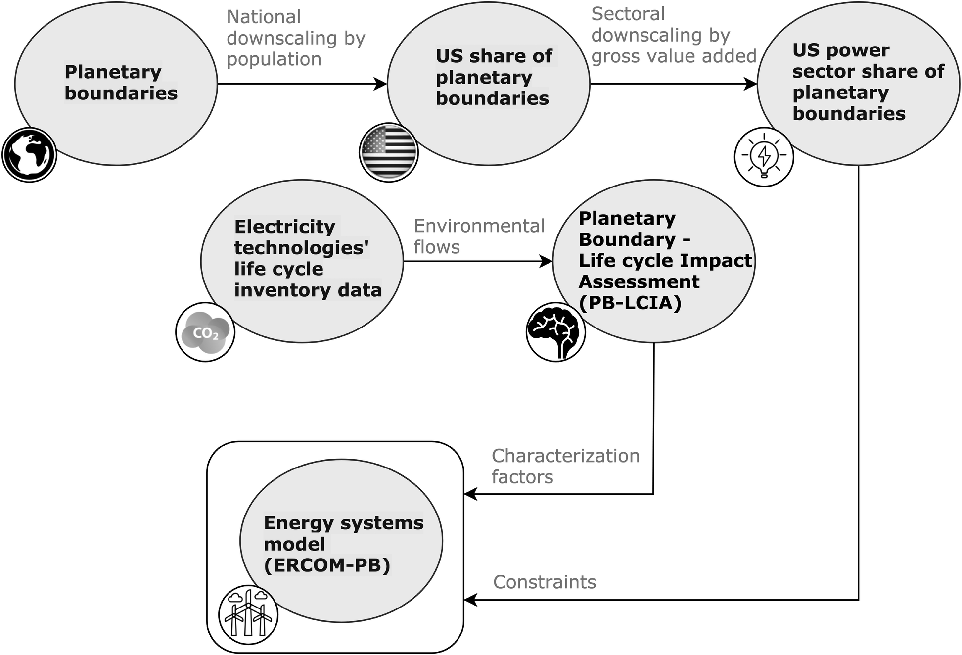 | ||
| Fig. 1 Modeling framework linking planetary boundaries with energy systems models. The PB-LCIA framework is based on published characterization factors that link life cycle inventories to Earth-system processes associated with planetary boundaries. | ||
Downscaling planetary boundaries to the sectoral level
PBs, defined at the global level, need to be downscaled first to the national and sectoral level to provide shares (i.e., an upper bound on the total impact) that shall be respected by the US power sector in 2030 (Fig. 1). Allocating shares of the safe operating space defined by the concept of PBs among countries and sectors is a controversial step, as it requires applying sharing principles on which no general agreement has been reached so far (e.g., sharing them equally among the world population21–23 or allocating them following tailored allocation procedures, such as expert judgment and past impacts24–26). Here, without loss of generality, we apply an egalitarian-based sharing principle,27 whereby the US power sector share of the safe operating space is quantified from the ratio of the US population to the global population times the ratio of the US power sector Gross Value Added (GVA) to the GVA of the whole US economy (Fig. 1) as follows: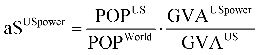 | (1) |
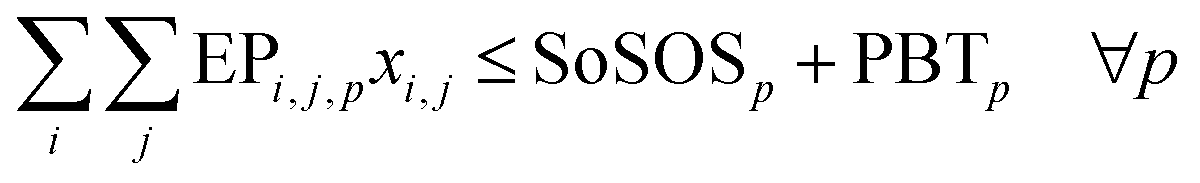
The share of the safe operating space, eqn (1), is then multiplied by the full safe operating space for every PB, yielding environmental bounds that are imposed in ERCOM-PB to ensure that the mix sought will not transgress any key ecological limit:
| SoSOSp = aSUSpower·SOSp ∀p | (2) |
| Planetary boundary title | Unit | Planetary boundary18 | Natural background level18,27 | Full safe operating space | Assigned share of safe operating space to the US power sector (aSUSpower = 0.062%) |
|---|---|---|---|---|---|
| a Planetary boundaries on stratospheric ozone depletion, ocean acidification and land-system change act as lower bounds18 and hence when the full safe operating space is calculated, the absolute value should be considered.27 | |||||
| Climate change (atmospheric CO2 concentration) | ppm CO2 | 350 | 278 | 72 | 0.045 |
| Climate change (energy imbalance at top-of-atmosphere) | W m−2 | 1 | 0 | 1 | 6.19 × 10⁻⁴ |
| Stratospheric ozone depletiona | DU | 275 | 290 | 15 | 0.009 |
| Ocean acidificationa | Ωarag | 2.75 | 3.44 | 0.69 | 4.27 × 10⁻⁴ |
| Biogeochemical phosphorus flow (global) | Tg P year−1 | 11 | 1.1 | 9.9 | 0.006 |
| Biogeochemical nitrogen flow (global) | Tg N year−1 | 62 | 0 | 62 | 0.038 |
| Land-system change (global)a | % | 75 | 100 | 25 | 0.015 |
| Freshwater use (global) | km3 year−1 | 4000 | 0 | 4000 | 2.476 |
Selection criteria for planetary boundaries in ERCOM-PB
Some PBs still show data and methodological gaps that prevent their full use in some practical application. Here, PBs relevant to the US energy systems were chosen based on (i) availability of the corresponding inventory entries in life cycle repositories; and (ii) applicability of the specific PB to our region of interest (i.e., the US). Based on the first criterion, the biosphere integrity PBs and the regional PBs on land-system change, freshwater use and biogeochemical Phosphorus (P) flow were omitted. Based on the second criterion, we discarded the PB on atmospheric aerosol loading, as the current PB focuses on the Indian subcontinent.18 Similarly, the PB on the introduction of novel entities was also omitted because it has not been formally defined yet.18 This leads to the consideration of eight out of fourteen global and regional PBs on seven out of ten ESPs already identified in the literature.18Linking life cycle inventories to planetary boundaries
Understanding and identifying the drivers of ESPs is the key that paves the way for the inclusion of PBs into ESMs. ESPs may seem ramified and difficult to reconcile in a single modeling environment, but a closer look delineates roots to cluster them into a number of environmental flows (or life cycle inventories) that could potentially be harnessed in environmental policies. These life cycle inventories are connected to ESPs via characterization factors recently proposed in the literature by Ryberg et al.28 as follows: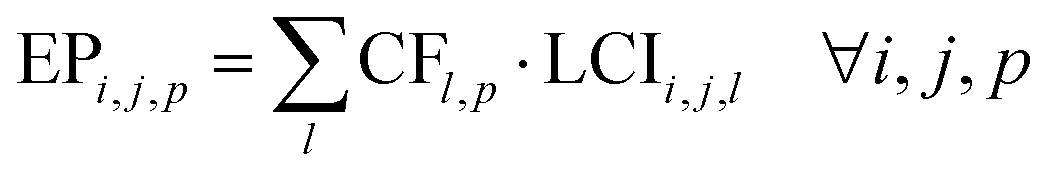 | (3) |
Two PBs, atmospheric CO2 concentration (ppm) and energy imbalance at top-of-atmosphere (W m−2), are used to describe climate change, which is responsible for both physical and biosphere fluctuations.17,18 GHG emissions such as CO2, CO, CH4 and NMVOC quantify the atmospheric CO2 concentration PB, while additional air emissions such as N2O, NF3, SF6, CFCs and HCFCs characterize in turn the energy imbalance PB.28
Stratospheric ozone depletion PB, measured in Dobson Unit (DU), evaluates the role of the ozone layer in filtering ultraviolet radiation from the Sun.17 Ozone depleting substances remove stratospheric ozone via reaction with chlorine and bromine;29 these include air emissions such as CFCs, HCFCs, Halons and R-40.28 Although the existing method to compute PBs28 does not assign a characterization factor that quantifies the N2O impact on the stratospheric ozone depletion PB, N2O emissions do exert a noticeable pressure on the ozone layer.30 Therefore, we here expand the existing method developed by Ryberg et al.28 by designing a characterization factor that quantifies the impact of N2O emissions on the stratospheric ozone depletion PB. In essence, we first convert the N2O emissions to CFC-11 equivalent (i.e., 0.018 kg of CFC-11 equivalent per kg of N2O)30 and then apply the characterization factor that links CFC-11 to the stratospheric ozone depletion PB available in the existing framework.28
The ocean acidification PB is measured in Ωarag. Since marine species are vulnerable to changes in the CO2 chemistry of oceans,17 this PB is closely related to the atmospheric CO2 concentration PB. An increasing concentration of CO2 in the ocean could raise its acidity causing many aragonite shells to dissolve.17 Ocean acidification mangles marine biodiversity and, therefore, it could affect the ability of oceans to sink CO2.17,18 Similar to the atmospheric CO2 concentration PB, though using different characterization factors, the ocean acidification PB is quantified via air emissions that include CO2, CO, CH4 and NMVOC.28
Freshwater eutrophication is connected to PBs that limit global biogeochemical P and Nitrogen (N) flows, measured in Tg P and Tg N, respectively.18 An excess amount of biogeochemical P and N flows induced by human interventions could disturb their global cycles,31,32 pushing marine systems across their tipping point.17 Global biogeochemical P flow is quantified from the P flow to freshwater; meanwhile, the biogeochemical N flow is obtained from NOx and NH3 to air, N-tot and NO3− to freshwater and NO3− to groundwater.28
Land-system change PB, expressed as a percentage of the original forest cover, evaluates the way in which climate is regulated through the exchange of energy and water between land and the atmosphere.18 The global PB on land-system change imposes a lower bound on the forest cover remaining area relative to the original forest cover.18 The land-system change PB is linked to the area of forest transformation associated with a given process.28
The freshwater use PB, measured in km3, limits the consumption of blue water.18,33 This PB reflects the vulnerability of biodiversity, food and health security to global manipulation of the freshwater cycle.17 When implementing this PB into an ESM, freshwater from rivers, lakes, reservoirs and groundwater should be considered to ensure consistency with the designed PB on freshwater use.18,33
To evaluate PBs, life cycle inventory entries, LCIi,j,l, connected to PBs were retrieved from the ecoinvent LCA database34,35 as well as from other specific technically sound sources36–39 (Table S1, ESI†). Published characterization factors, CFl,p, were applied to translate the life cycle inventories of electricity technologies into the environmental burdens, EPi,j,p, linked to PBs (eqn (3)).28
The emissions reduction cooperation model with planetary boundaries
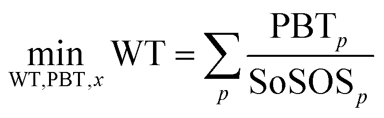
The PBs mentioned previously were incorporated into ERCOM,6 an ESM tailored to the US that minimizes the electricity cost for a given target on emissions, imposed either at the national or state level. The new model, referred to as ERCOM-PB, incorporates PBs and assumes full cooperation among states – that is, the US operates as a single entity to satisfy the domestic electricity demand while meeting a national environmental target. ERCOM-PB is formulated as a linear programming model that finds the least cost pathway (i.e., electricity mix) minimizing the total transgression of downscaled PBs to the US power sector, while considering technical constraints relevant to energy mixes.The model is outlined next, while a full description of ERCOM-PB and the corresponding data sources is available in Notes S1, S2 and Table S1 (ESI†). Furthermore, the uncertainty analysis approach is described in Note S3 (ESI†), while the main limitations of our modeling framework are summarized in Note S4 (ESI†).
ERCOM-PB can be expressed in compact form as follows:
 | (4) |
| PBTp ≥ 0 ∀p | (5) |
 | (6) |
| Ai,jxi,j ≤ ai,j ∀i,j | (7) |
WT, PBT, x ∈ ![[Doublestruck R]](https://www.rsc.org/images/entities/char_e175.gif) | (8) |
is the set of real numbers to which variables WT, PBTp and xi,j belong.
Solutions definition
To underscore the importance of incorporating PBs in designing sustainable energy mixes, we analyze three electricity mixes that meet the expected electricity demand in 2030 (Table 2). The ‘BAU’ solution (S1) represents the US 2012 default developments in the power sector to meet the 2030 electricity demand (i.e., the same breakdown of technologies as in 2012 would be implemented to cover the energy demand in 2030). The ‘Paris Agreement’ solution (S2) corresponds to the least cost solution that meets the US commitment to the Paris Agreement 2 °C target in 2030 while satisfying the same electricity demand as in the BAU solution. To obtain this mix, we solved a slight variant model of ERCOM-PB, where objective function (9) replaces objective function (4) and inequality (10) replaces inequalities (5) and (6) as follows: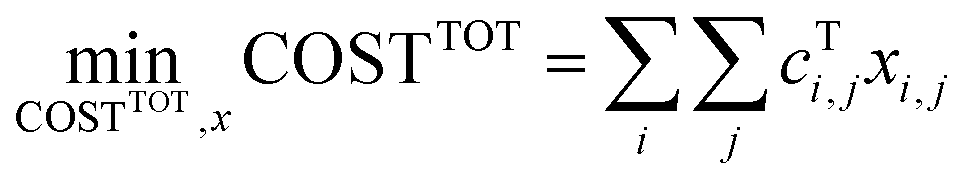 | (9) |
 | (10) |
| Ai,jxi,j ≤ ai,j ∀i,j | (11) |
| COSTTOT, x ∈ | (12) |
| Solution title | Solution label | Description |
|---|---|---|
| Business as usual | S1 | The 2012 energy mix in 2030, where the share of each technology is fixed to its 2012 level and the demand is projected to 2030 |
| Paris Agreement | S2 | The energy mix in 2030 that would meet the US commitment to the Paris Agreement 2 degrees Celsius target and the projected demand in 2030 at minimum cost |
| Planetary boundaries | S3 | The energy mix in 2030 that would minimize the transgression of planetary boundaries at minimum cost |
Finally, the ‘Planetary boundaries’ solution (S3) is obtained as follows. We first solve ERCOM-PB (4)–(8) to find the solution with the smallest transgression of PBs. As cost is not accounted for in the objective function, the model could find solutions with the same level of transgression but less costly that would be, therefore, more appealing for decision-makers. Hence, in a subsequent step, we fix the amount by which PBs are transgressed in the optimal solution of ERCOM-PB (i.e., the minimum transgression possible among all the electricity mixes satisfying the technical constraints and meeting the demand) and minimize the total cost (eqn (9)), finding solution S3.
Results and discussion
Myopic policies to planetary boundaries
We start by analyzing the US electricity mix in the BAU solution (S1) through the lens of PBs (Fig. 2). We assumed the most stringent PBs values as suggested by Steffen et al.18 and considered the main uncertainties associated with the environmental burdens (i.e., life cycle inventory entries) connected to PBs as well as with the LCOE values of electricity technologies (Note S3, ESI†). The results of the uncertainty analysis of the environmental burdens are reported in the figures as error bars, where each error bar represents one standard deviation.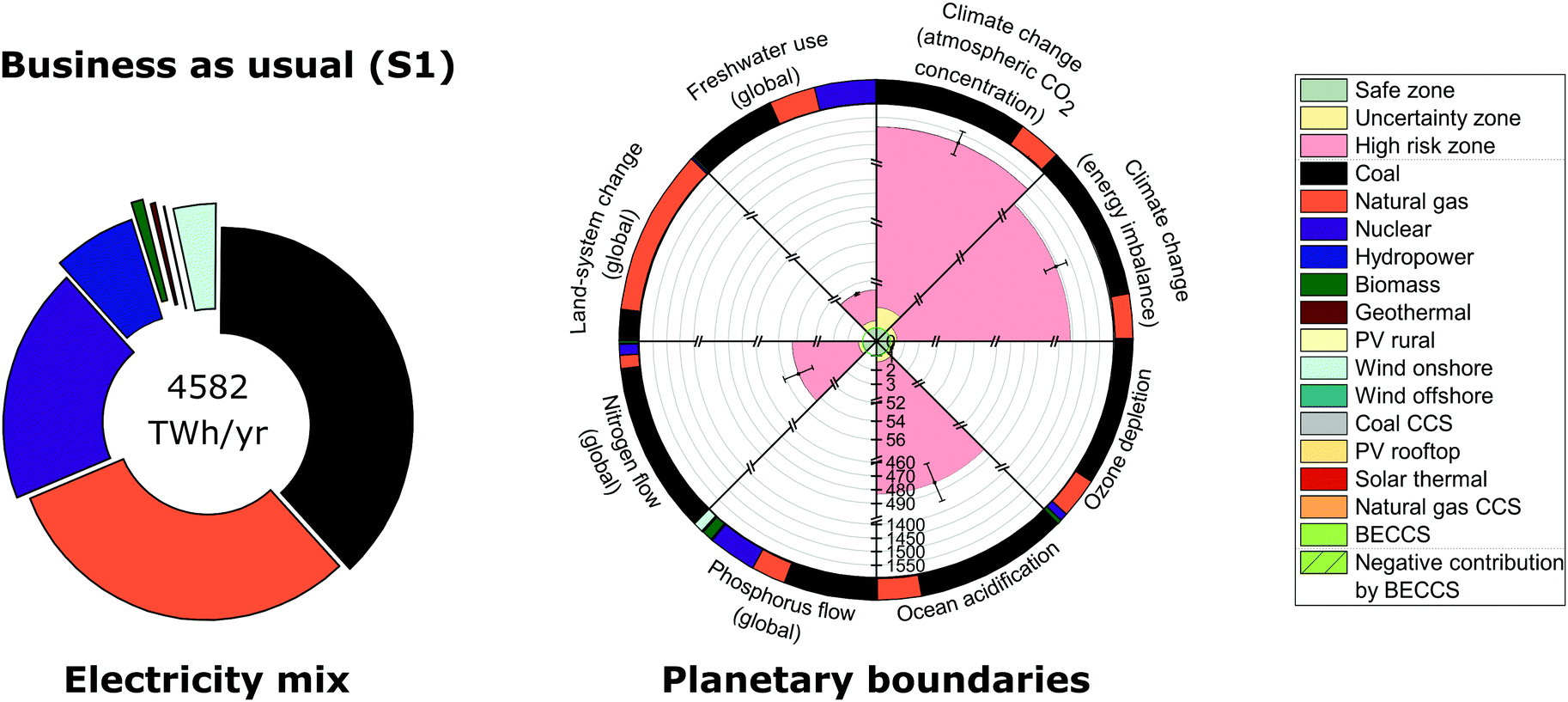 | ||
| Fig. 2 Global US electricity generation and imports portfolio and performance relative to downscaled planetary boundaries for the business as usual energy mix (solution S1). The circle on the left represents the 2012 energy mix in 2030; its performance in terms of planetary boundaries is summarized in a rose chart on the right. The rose chart represents the current performance of each Earth-system process divided by the US power sector share of the full safe operating space (i.e., a value less than one implies it lies below the planetary boundary). The green zone is the safe operating space (i.e., within the strictest planetary boundary in the uncertainty range), the yellow zone is the uncertainty range of each planetary boundary and the red zone is beyond the least strict planetary boundary in the uncertainty range. Each error bar corresponds to one standard deviation considering the uncertainty in environmental burdens (i.e., life cycle inventory entries) connected to planetary boundaries. Each circular sector of the outer ring on the right represents the intensity of each technology on each planetary boundary. The labeling of solutions is given in Table 2. | ||
We found that six out of the eight PBs considered are transgressed in solution (S1), including atmospheric CO2 concentration, energy imbalance at top-of-atmosphere, ocean acidification, biogeochemical N flow, freshwater use and stratospheric ozone depletion (Fig. 2), which raises significant concerns about our future ability to deliver sustainable energy without altering the current status quo. Only two PBs would hence be satisfied, namely biogeochemical P flow and land-system change.
Though the transgression of the PB on stratospheric ozone depletion is within the uncertainty zone (i.e., the yellow zone in Fig. 2), the remaining transgressed PBs in the BAU mix fall beyond the uncertainty zone (i.e., the red high risk zone in Fig. 2), indicating there is certainty in failing to operate within the Earth's safe operating space. PBs on climate change are transgressed the most; the PB on atmospheric CO2 concentration is transgressed by 1515 times above the limit, while energy imbalance at top-of-atmosphere is transgressed by 1442 times above the limit. They are followed by ocean acidification, transgressed by 483 times above the limit. Analyzing the contribution of the electricity technologies to PBs, we found that the deployment of coal and natural gas power plants seem to be the main reason behind the transgression of the climate change PBs and the PB on ocean acidification (Fig. 2). At a lesser transgression extent, the global PB on biogeochemical N flow is surpassed by 55 times above the limit, mainly due to the reliance on coal power plants. Moreover, freshwater use transgresses the limit by fourfold due to the deployment of coal, nuclear and natural gas power plants. Finally, stratospheric ozone depletion is transgressed the least (i.e., 18% above the limit) mainly due to the reliance on coal power plants and, albeit to a lesser extent, natural gas plants.
We next analyze solution S2, that is, the grid that would emerge from the cost minimization of the US mix considering a limit on GHG emissions; to this end, we used the GWP100 in line with the US Intended Nationally Determined Contribution (INDC) under the Paris Agreement 2 °C target. The US INDC commits the nation to reduce its GWP100 by 26–28% in 2025 (or around 39% in 2030) compared to the 2005 levels.41 Note that due to electricity transmission losses between neighboring regions, the electricity generated in solution S2 differs from that in solution S1. In terms of the mix that would emerge in solution S2, we found that the Paris Agreement mix would displace primarily coal power plants by renewables, particularly wind onshore (Fig. 3). In fact, even after enforcing the Paris Agreement target (S2), only one additional PB, namely the one on stratospheric ozone depletion, is met compared to the BAU mix (S1) due to the displacement of coal power plants – five out of the eight PBs considered would still be transgressed. The transgressed PBs in solution S2 include both PBs on climate change, as well as PBs on ocean acidification, biogeochemical N flow and freshwater use.
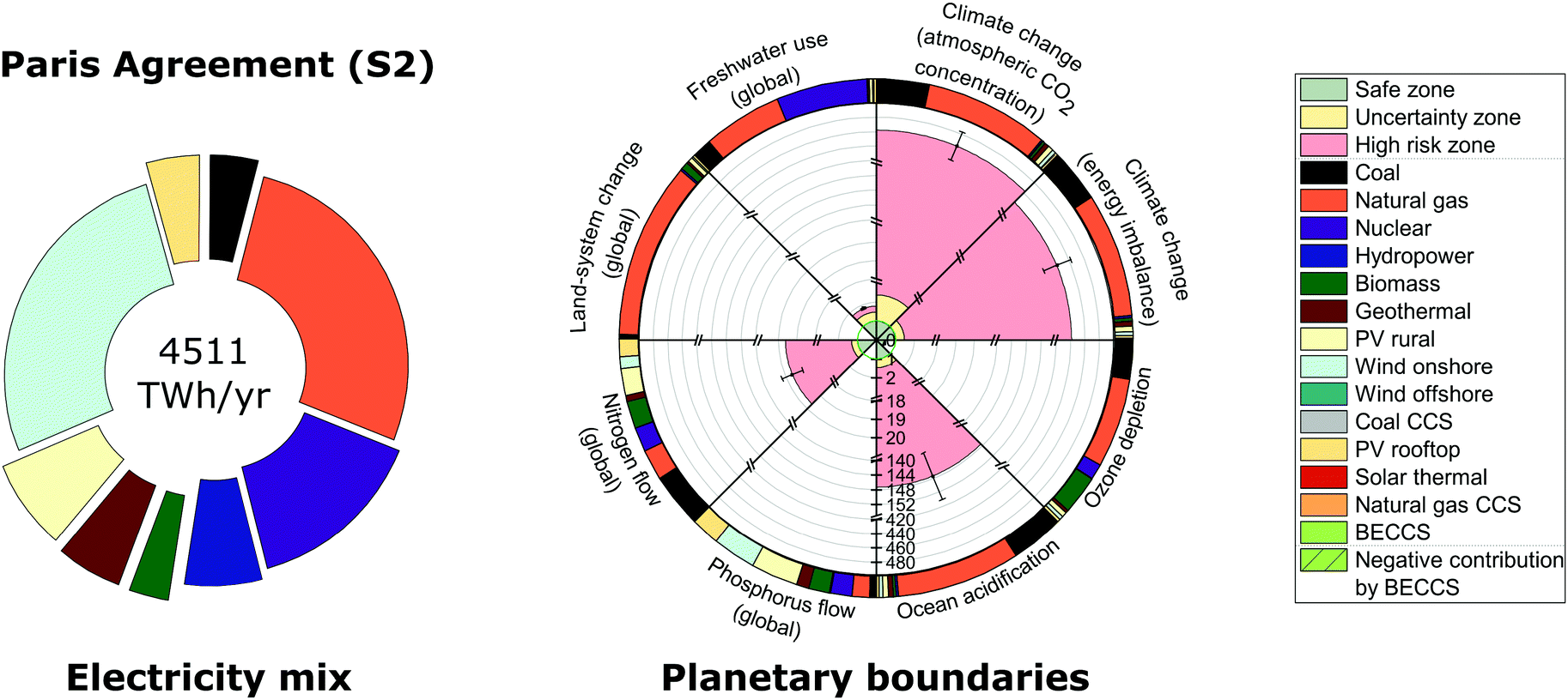 | ||
| Fig. 3 Global US electricity generation and imports portfolio and performance relative to downscaled planetary boundaries for the Paris Agreement mix (solution S2). The circle on the left represents the energy mix in 2030 that meets the Paris Agreement 2 degrees Celsius target at minimum cost; its performance in terms of planetary boundaries is summarized in a rose chart on the right. The rose chart represents the current performance of each Earth-system process divided by the US power sector share of the full safe operating space (i.e., a value less than one implies it lies below the planetary boundary). The green zone is the safe operating space (i.e., within the strictest planetary boundary in the uncertainty range), the yellow zone is the uncertainty range of each planetary boundary and the red zone is beyond the least strict planetary boundary in the uncertainty range. Each error bar corresponds to one standard deviation considering the uncertainty in environmental burdens (i.e., life cycle inventory entries) connected to planetary boundaries. Each circular sector of the outer ring on the right represents the intensity of each technology on each planetary boundary. The labeling of solutions is given in Table 2. | ||
The Paris Agreement mix (S2) would reduce the transgression of every PB ranging from 49 to 69% in contrast to the BAU mix (S1); however, the five transgressed PBs would still lie in the PBs high risk zone (the red zone in Fig. 3). In fact, both PBs on atmospheric CO2 concentration and energy imbalance at top-of-atmosphere are transgressed by 462 and 442 times above the limit, respectively, as both PBs on climate change are more stringent than the Paris Agreement 2 °C target. The PB on ocean acidification is also transgressed by 147 times above the limit. Similar to the BAU mix, the reliance of solution S2 on natural gas and, to a lesser extent, coal power plants contribute to the transgression of the climate change PBs and the PB on ocean acidification (Fig. 3). Furthermore, solution S2 transgresses the PB on biogeochemical N flow by 20 times above the limit due to the deployment of coal, biomass and PV plants. Lastly, the freshwater use PB is transgressed by two times above the limit due to the deployment of nuclear, coal and natural gas power plants.
Minimizing the transgression of planetary boundaries
ERCOM-PB is next solved aiming to satisfy all PBs simultaneously (solution S3 shown in Fig. 4). We found that no energy mix exists that can meet all of the PBs concurrently. More precisely, no single energy mix can satisfy the global biogeochemical N flow PB, noting that in this PB, solution S3 lies in the high risk zone (red area in Fig. 4).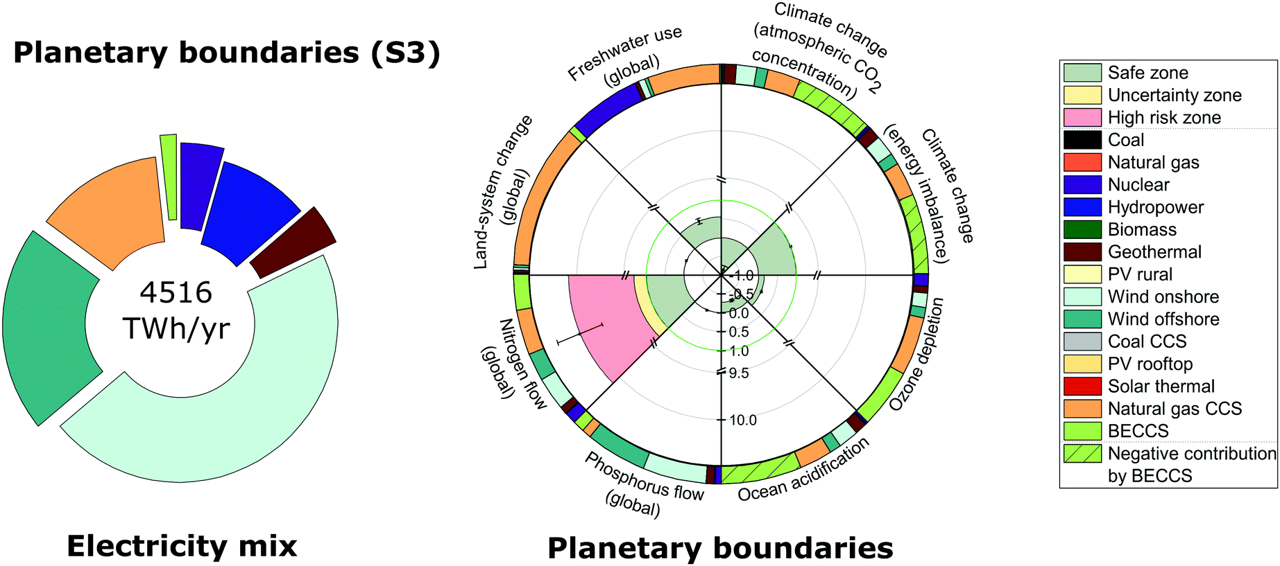 | ||
| Fig. 4 Global US electricity generation and imports portfolio and performance relative to downscaled planetary boundaries for the planetary boundaries mix (solution S3). The circle on the left represents the energy mix in 2030 that would minimize the transgression of planetary boundaries at minimum cost; its performance in terms of planetary boundaries is shown in a rose chart on the right. The rose chart represents the current performance of each Earth-system process divided by the US power sector share of the full safe operating space (i.e., a value less than one implies it lies below the planetary boundary). The green zone is the safe operating space (i.e., within the strictest planetary boundary in the uncertainty range), the yellow zone is the uncertainty range of each planetary boundary and the red zone is beyond the least strict planetary boundary in the uncertainty range. Each error bar corresponds to one standard deviation considering the uncertainty in environmental burdens (i.e., life cycle inventory entries) connected to planetary boundaries. Each circular sector of the outer ring on the right represents the intensity of each technology on each planetary boundary. The labeling of solutions is given in Table 2. | ||
The mix in solution S3 reduces the number of coal and natural gas plants while deploying BECCS, wind onshore and offshore and natural gas with CCS power plants; this allows the mix to meet both PBs on climate change as well as the PB on ocean acidification (Fig. 4). Overall, solution S3 shows a net negative contribution towards both PBs on atmospheric CO2 concentration and ocean acidification, mainly due to the deployment of BECCS, a net negative emission technology on a life cycle basis.39 On the other hand, the energy imbalance PB assigns larger weights to CFCs and other GHG emissions compared to CO2; consequently, BECCS shows a lower net negative contribution in this category (Note S5 and Fig. S1, ESI†). Overall, the deployment of low (or negative) GHG emissions technologies (on a life cycle basis) allows the mix to meet the PB on energy imbalance at top-of-atmosphere.
Solution S3 meets the freshwater use PB by partially displacing natural gas and nuclear plants while completely phasing out coal plants. Furthermore, the deployment of hydropower and wind onshore and offshore plants reduces the transgression of the global biogeochemical N flow PB by 49% compared to the Paris Agreement mix (S2) and 81% compared to the BAU mix (S1). In solution S3, this transgression is mainly due to the deployment of BECCS and natural gas with CCS plants as well as the presence of nuclear plants.
The contribution of major environmental flows (i.e., life cycle inventories) towards the performance of each solution in every PB is shown in Note S5 and Fig. S1 (ESI†), where it becomes clear that each PB is mainly originated by a handful of key environmental flows.
Economic implications of planetary boundaries
To understand the economic implications of meeting several PBs, we next compare the total US cost of electricity in solutions S1, S2 and S3 (Fig. 5). The Paris Agreement mix (S2) is less expensive than the BAU mix (S1), mainly due to the future economic competitiveness of the LCOE values of renewable technologies, particularly wind onshore and geothermal, in contrast to conventional power plants (Table S2, ESI†).40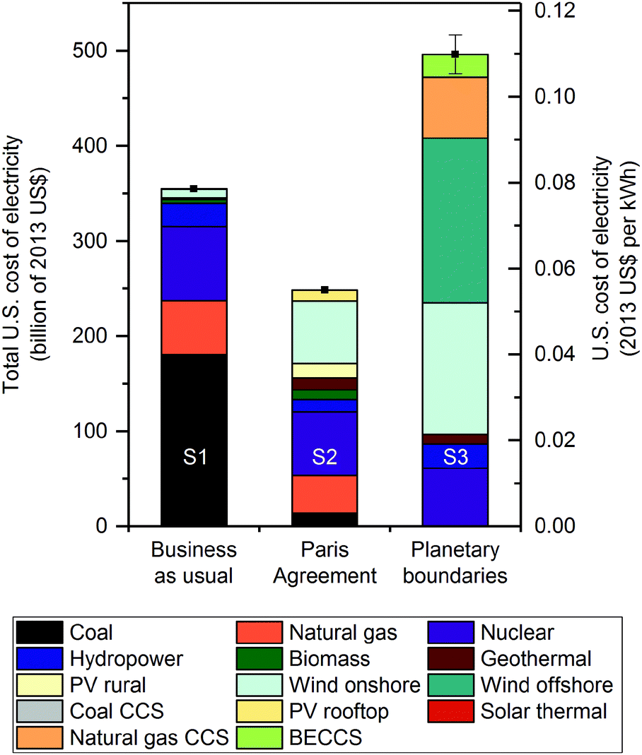 | ||
| Fig. 5 US optimal cost of electricity generation and imports in 2030 broken by technology. The primary y-axis denotes the total cost of electricity supply and the secondary y-axis represents the average cost of electricity in USD2013 per kWh. The business as usual energy mix, solution S1, (column on the left) represents an energy mix with the same technological breakdown as in 2012 but meeting the projected demand in 2030. The Paris Agreement mix, solution S2, (column on the center) represents the least cost energy mix in 2030 that would meet the Paris Agreement 2 degrees Celsius target. The planetary boundaries mix, solution S3, (column on the right) represents the least cost energy mix in 2030 that would minimize the transgression of planetary boundaries. Each error bar corresponds to one standard deviation due to the uncertainty in environmental burdens (i.e., life cycle inventory entries) connected to planetary boundaries. The labeling of solutions is given in Table 2. | ||
The least cost solution that minimizes the transgression of PBs (S3) has the drawback of increasing the cost of electricity by 40% compared to the BAU mix (S1) while doubling the cost compared to the Paris Agreement mix (S2) (Fig. 5). The differences in costs incurred by solution S3 in contrast to the BAU (S1) and Paris Agreement (S2) mixes constitute 0.8% and 1.3%, respectively, of the US GDP in 2017. This extra cost is mainly due to the deployment of wind offshore, natural gas with CCS and BECCS, at present more expensive than other renewable technologies (e.g., wind onshore and geothermal). The Paris Agreement mix is also cost optimal when no bounds on emissions are imposed, which highlights the economic40 (in addition to environmental) benefits of meeting the Paris Agreement 2 °C target.
Uncertainties associated with the future LCOE values, which are more pronounced in emerging technologies (e.g., BECCS) than in conventional ones (Table S2, ESI†),42 are analyzed in Note S6 (ESI†). We note that emerging technologies are found to be necessary by ERCOM-PB to meet seven PBs concurrently (Fig. S2, ESI†); consequently, their uncertain LCOE values need to be properly assessed. Our analysis shows that these uncertainties associated with emerging technologies (e.g., BECCS) deployed in solution S3 do not change substantially our economic results (Note S6 and Fig. S2, ESI†).
Furthermore, acknowledging that future LCOE values of emerging technologies might be critically affected by learning curves, we also performed a post-optimal uncertainty analysis of solutions S1 and S2 by varying the LCOE values of electricity technologies from the current levels43 to the future ones40 (Table S3, ESI†), where the latter values consider the expected potential technological development. Results reveal that the probability of the Paris Agreement mix (S2) being more expensive than the BAU mix (S1) is rather low (i.e., 5%) (Note S7 and Fig. S3, ESI†). This is mainly due to the fact that electricity technologies performing very well in PBs (e.g., wind onshore and geothermal) are also cost advantageous in the future compared to technologies dominating currently the BAU mix (Table S3, ESI†).
Conclusions
Our results have strong implications for both policymaking and research on energy systems design. First, we found that the current US policy framework, solution S2, would ‘lock in’44 a plan that would not meet all PBs concurrently despite the attainment of the Paris Agreement 2 °C target; this finding reinforces the need to take action to keep our Earth within its ecological limits. Power plants are capital-intense investments, thus dismantling plants is seldom favorable. Therefore, designing early, comprehensive and strategic policies that could maintain our growing demand for energy without transgressing PBs is crucial for attaining sustainable development.Wind onshore and offshore, natural gas with CCS and BECCS play a key role in meeting concurrently seven of the eight PBs considered in the US, while minimizing the transgression of the remaining PB on biogeochemical N flow. In fact, the ability to deploy negative emission technologies (e.g., BECCS) in the power sector would provide some degree of flexibility in meeting the total atmospheric CO2 concentration and ocean acidification PBs at the global level, as the power sector could offset, to some extent, the contribution of other worse-endowed sectors to these PBs. Nonetheless, with the current technological landscape in the US power sector, meeting the global biogeochemical N flow seems unattainable; this is due to the limited potential of those technologies that are competitive across all PBs, such as hydropower and wind technologies. Pathways that could improve the current potential and reliability of hydropower and wind technologies through, for example, the deployment of more affordable storage facilities45,46 could aid meeting all of the PBs concurrently.
Alternatively, sectors (and also countries) could trade shares of PBs so one sector (or country) could operate under more stringent targets in those PBs easier to meet, while performing worse in those harder to satisfy. For example, the poor performance of energy systems in terms of biogeochemical N flow could be offset to some extent by imposing more stringent targets on other economic sectors with potential for offsetting such impact. Particularly, the power sector could exert a net negative contribution towards atmospheric CO2 concentration and ocean acidification by deploying BECCS, which would allow the sector to ‘trade’ shares of other PBs, mainly biogeochemical N flow, with other sectors. Nonetheless, this would ultimately require mechanisms to share burdens across sectors following some principles, which should consider the sectoral contributions to the population's well-being.
The reliance on expensive technologies (e.g., wind offshore, natural gas with CCS and BECCS) needed to meet seven of the eight PBs while minimizing the transgression of the biogeochemical N flow PB would increase the cost of electricity generation, 40% relative to the BAU solution and 100% relative to the Paris Agreement solution. These additional costs relative to the BAU and Paris Agreement mixes would constitute 0.8% and 1.3% of the US GDP in 2017, respectively. Therefore, further research to decrease the LCOE of such technologies is needed to dampen the cost of meeting PBs. In this context, other negative emissions technologies, such as Direct Air Capture (DAC),47 could also be incorporated in ERCOM-PB. We keep the exploration of this idea as part of our future work due to the current limited availability of projected economic and technical data to the future of other negative emissions technologies.
We note that significant uncertainties are involved in the calculation of some PBs. For instance, the uncertainty range of the PB on the global P flow is a factor of ten, while the uncertainty range of the PB on ozone depletion is a factor of two.18 Narrowing the PB uncertainty ranges would have implications on the cost of generating sustainable electricity. For example, imposing less strict PBs on ESPs that are difficult to meet by the US power sector, such as climate change, could deploy less expensive electricity technologies and hence reduce the cost of electricity supply. Therefore, these uncertainties should be studied thoroughly to produce more robust planetary targets and to design sustainable energy systems and policies accordingly.
Finally, urgent research is needed to design characterization factors that link life cycle inventory entries to the PBs on the two ESPs overlooked so far, namely biosphere integrity and introduction of novel entities. Similarly, characterization models need to be designed to connect life cycle inventory entries readily available in LCA repositories (e.g., ecoinvent34,35) to regional PBs. Lastly, global PBs on atmospheric aerosol loading and introduction of novel entities need to be quantified to sustain their safe operating space zones.
Nomenclature
| BAU | Business as usual |
| BECCS | Bio-energy with carbon capture and storage |
| CCS | Carbon capture and storage |
| DAC | Direct air capture |
| ERCOM | Emissions reduction cooperation model |
| ERCOM-PB | Emissions reduction cooperation model with planetary boundaries |
| ESM | Energy systems model |
| ESO | Electricity systems optimization |
| ESP | Earth-system process |
| GDP | Gross domestic product |
| GHG | Greenhouse gas |
| GVA | Gross value added |
| GWP100 | 100-year global warming potential |
| INDC | Intended nationally determined contribution |
| LCA | Life cycle assessment |
| LCOE | Levelized cost of electricity |
| N | Nitrogen |
| P | Phosphorus |
| PB | Planetary boundary |
Indices
| i | Electricity generation technology |
| j | State |
| p | Planetary boundary |
Sets
| Real numbers |
Parameters
| A i,j | Technical matrix of constraints for technology i in state j |
| a i,j | Upper bound vector for technology i in state j |
| aSUSpower | Assigned share of the full safe operating space to the power sector in the United States |
| c T i,j | Cost of electricity generation for technology i in state j |
| CFl,p | Characterization factor that links life cycle inventory entry l to planetary boundary p |
| EPi,j,p | Environmental burden linked to planetary boundary p per unit of energy supplied by technology i in state j |
| GVAUS | United States total gross value added |
| GVAUSpower | United States power sector gross value added |
| GWP100i,j | 100-year global warming potential per unit of energy generated by technology i in state j |
| LCIi,j,l | Life cycle inventory l generated when one unit of electricity is supplied via technology i in state j |
| POPUS | United States population |
| POPWorld | World population |
| SOSp | Full safe operating space for planetary boundary p |
| SoSOSp | United States power sector absolute share of the full safe operating space for planetary boundary p |
| TARG | 100-year global warming potential target in line with the United States commitment to the Paris Agreement 2 degrees Celsius target in 2030 |
Variables
| COSTTOT | Total cost of electricity supply |
| WT | Total weighted transgression of planetary boundaries by the United States power sector share of the safe operating space |
| PBTp | Transgression of downscaled planetary boundary p |
| x i,j | Electricity generated by technology i in state j |
Conflicts of interest
There are no conflicts to declare.Acknowledgements
I. M. A. thanks Saudi Aramco for the full PhD scholarship. G. G.-G. acknowledges the Spanish Ministry of Education and Competitiveness (CTQ2016-77968-C3-1-P, MINECO/FEDER) for the financial support received. C. P., G. G.-G. and N. M. D. acknowledge the financial support from NERC – Natural Environment Research Council (NE/P019900/1). M. A. J. H. was supported by an ERC consolidation grant (ERC – CoG SIZE 647224).References
- R. Loulou, G. Goldstein and K. Noble, Energy Technology Systems Analysis Programme, 2004, pp. 65–73 Search PubMed.
- EIA, The Electricity Market Module of the National Energy Modeling System: Model Documentation, US Energy Information Administration, 2011. https://www.eia.gov/outlooks/aeo/nems/documentation/electricity/pdf/m068(2011).pdf.
- M. Fripp, Environ. Sci. Technol., 2012, 46, 6371–6378 CrossRef CAS PubMed.
- J. Nelson, J. Johnston, A. Mileva, M. Fripp, I. Hoffman, A. Petros-Good, C. Blanco and D. M. Kammen, Energy Policy, 2012, 43, 436–447 CrossRef.
- C. F. Heuberger, E. S. Rubin, I. Staffell, N. Shah and N. Mac Dowell, Appl. Energy, 2017, 204, 831–845 CrossRef.
- A. Galan-Martin, C. Pozo, A. Azapagic, I. E. Grossmann, N. Mac Dowell and G. Guillen-Gosalbez, Energy Environ. Sci., 2018, 11, 572–581 RSC.
- M. Zeyringer, J. Price, B. Fais, P. H. Li and E. Sharp, Nat. Energy, 2018, 3, 395–403 CrossRef CAS.
- S. Pye, F. G. N. Li, J. Price and B. Fais, Nat. Energy, 2017, 2, 17024 CrossRef.
- C. F. Heuberger, I. Staffell, N. Shah and N. Mac Dowell, Nat. Energy, 2018, 3, 634–640 CrossRef.
- J. Rockstrom, O. Gaffney, J. Rogelj, M. Meinshausen, N. Nakicenovic and H. J. Schellnhuber, Science, 2017, 355, 1269–1271 CrossRef PubMed.
- D. Garcia-Gusano, I. R. Istrate and D. Iribarren, Sci. Total Environ, 2018, 612, 386–391 CrossRef CAS PubMed.
- M. Pehl, A. Arvesen, F. Humpenoder, A. Popp, E. G. Hertwich and G. Luderer, Nat. Energy, 2017, 2, 939–945 CrossRef CAS.
- S. Rauner and M. Budzinski, Environ. Res. Lett., 2017, 12, 124005 CrossRef.
- P. Limleamthong and G. Guillen-Gosalbez, J. Cleaner Prod., 2017, 164, 1602–1613 CrossRef.
- M. Child, O. Koskinen, L. Linnanen and C. Breyer, Renewable Sustainable Energy Rev., 2018, 91, 321–334 CrossRef.
- J. Rockstrom, W. Steffen, K. Noone, A. Persson, F. S. Chapin, E. F. Lambin, T. M. Lenton, M. Scheffer, C. Folke, H. J. Schellnhuber, B. Nykvist, C. A. de Wit, T. Hughes, S. van der Leeuw, H. Rodhe, S. Sorlin, P. K. Snyder, R. Costanza, U. Svedin, M. Falkenmark, L. Karlberg, R. W. Corell, V. J. Fabry, J. Hansen, B. Walker, D. Liverman, K. Richardson, P. Crutzen and J. A. Foley, Nature, 2009, 461, 472–475 CrossRef PubMed.
- J. Rockstrom, W. Steffen, K. Noone, A. Persson, F. S. Chapin, E. Lambin, T. M. Lenton, M. Scheffer, C. Folke, H. J. Schellnhuber, B. Nykvist, C. A. de Wit, T. Hughes, S. van der Leeuw, H. Rodhe, S. Sorlin, P. K. Snyder, R. Costanza, U. Svedin, M. Falkenmark, L. Karlberg, R. W. Corell, V. J. Fabry, J. Hansen, B. Walker, D. Liverman, K. Richardson, P. Crutzen and J. Foley, Ecology and Society, 2009, 14, 32 CrossRef.
- W. Steffen, K. Richardson, J. Rockstrom, S. E. Cornell, I. Fetzer, E. M. Bennett, R. Biggs, S. R. Carpenter, W. de Vries, C. A. de Wit, C. Folke, D. Gerten, J. Heinke, G. M. Mace, L. M. Persson, V. Ramanathan, B. Reyers and S. Sorlin, Science, 2015, 347, 1259855 CrossRef PubMed.
- R. W. Kates, T. M. Parris and A. A. Leiserowitz, Environment, 2005, 47, 8–21 Search PubMed.
- D. Griggs, M. Stafford-Smith, O. Gaffney, J. Rockstrom, M. C. Ohman, P. Shyamsundar, W. Steffen, G. Glaser, N. Kanie and I. Noble, Nature, 2013, 495, 305–307 CrossRef CAS PubMed.
- D. W. O'Neill, A. L. Fanning, W. F. Lamb and J. K. Steinberger, Nature Sustainability, 2018, 1, 88–95 CrossRef.
- B. Nykvist, National environmental performance on planetary boundaries: a study for the Swedish Environmental Protection Agency, Report 9162065769, Swedish Environmental Protection Agency, 2013. https://www.naturvardsverket.se/Documents/publikationer6400/978-91-620-6576-8.pdf.
- H. Hoff, B. Nykvist and M. Carson, SEI Working Paper, 2014, 2014-05.
- M. J. Cole, R. M. Bailey and M. G. New, Proc. Natl. Acad. Sci. U. S. A., 2014, 111, E4399–E4408 CrossRef CAS PubMed.
- H. Y. Teah, T. Akiyama, R. S. Carlos, O. V. Rayo, Y. T. J. Khew, S. J. Zhao, L. F. Zheng and M. Onuki, Sustainability, 2016, 8, 1233 CrossRef.
- T. Häyhä, P. L. Lucas, D. P. van Vuuren, S. E. Cornell and H. Hoff, Global Environmental Change, 2016, 40, 60–72 CrossRef.
- M. W. Ryberg, M. Owsianiak, J. Clavreul, C. Mueller, S. Sim, H. King and M. Z. Hauschild, Sci. Total Environ, 2018, 634, 1406–1416 CrossRef CAS PubMed.
- M. W. Ryberg, M. Owsianiak, K. Richardson and M. Z. Hauschild, Ecol. Indic., 2018, 88, 250–262 CrossRef.
- D. W. Fahey and M. I. Hegglin, Twenty Questions and Answers about the Ozone Layer 2010 Update: Scientific Assessment of Ozone Depletion 2010, World Meteorological Organisation, 2011.
- J. Lane and P. Lant, Int. J. Life Cycle Assess., 2012, 17, 252–257 CrossRef CAS.
- N. Gruber and J. N. Galloway, Nature, 2008, 451, 293–296 CrossRef CAS PubMed.
- F. T. Mackenzie, L. M. Vera and A. Lerman, Chem. Geol., 2002, 190, 13–32 CrossRef CAS.
- M. Falkenmark, Philos. Trans. R. Soc., B, 1997, 352, 929–936 CrossRef.
- G. Wernet, C. Bauer, B. Steubing, J. Reinhard, E. Moreno-Ruiz and B. Weidema, Int. J. Life Cycle Assess., 2016, 21, 1218–1230 CrossRef.
- R. Frischknecht, N. Jungbluth, H.-J. Althaus, G. Doka, R. Dones, T. Heck, S. Hellweg, R. Hischier, T. Nemecek and G. Rebitzer, Int. J. Life Cycle Assess., 2005, 10, 3–9 CrossRef CAS.
- D. Iribarren, F. Petrakopoulou and J. Dufour, Energy, 2013, 50, 477–485 CrossRef CAS.
- B. Corona, G. San Miguel and E. Cerrajero, Int. J. Life Cycle Assess., 2014, 19, 1264–1275 CrossRef CAS.
- F. Petrakopoulou, D. Iribarren and J. Dufour, Greenhouse Gases: Sci. Technol., 2015, 5, 268–276 CrossRef CAS.
- G. D. Oreggioni, B. Singh, F. Cherubini, G. Guest, C. Lausselet, M. Luberti, H. Ahn and A. H. Stromman, Int. J. Greenhouse Gas Control, 2017, 57, 162–172 CrossRef CAS.
- EIA, Annual Energy Outlook 2015 with projections to 2040, 2015. https://www.eia.gov/outlooks/archive/aeo15/pdf/electricity_generation.pdf.
- UNFCCC, United States intended nationally determined contribution under the Paris Agreement, United Nations Framework Convention on Climate Change, 2015. https://www4.unfccc.int/sites/ndcstaging/PublishedDocuments/United%20States%20of%20America%20First/U.S.A.%20First%20NDC%20Submission.pdf.
- B. S. Koelbl, M. A. van den Broek, B. J. van Ruijven, A. P. C. Faaij and D. P. van Vuuren, Int. J. Greenhouse Gas Control, 2014, 27, 81–102 CrossRef CAS.
- EIA, 2016 Levelized Cost of New Generation Resources from the Annual Energy Outlook 2010, 2010. https://www.eia.gov/outlooks/archive/aeo10/pdf/2016levelized_costs_aeo2010.pdf.
- K. Riahi, E. Kriegler, N. Johnson, C. Bertram, M. Den Elzen, J. Eom, M. Schaeffer, J. Edmonds, M. Isaac and V. Krey, Technol. Forecase. Soc., 2015, 90, 8–23 CrossRef.
- C. F. Heuberger, I. Staffell, N. Shah and N. Mac Dowell, Comput. Chem. Eng., 2017, 107, 247–256 CrossRef CAS.
- C. F. Heuberger, I. Staffell, N. Shah and N. Mac Dowell, Energy Environ. Sci., 2016, 9, 2497–2510 RSC.
- M. Bui, C. S. Adjiman, A. Bardow, E. J. Anthony, A. Boston, S. Brown, P. S. Fennell, S. Fuss, A. Galindo, L. A. Hackett, J. P. Hallett, H. J. Herzog, G. Jackson, J. Kemper, S. Krevor, G. C. Maitland, M. Matuszewski, I. S. Metcalfe, C. Petit, G. Puxty, J. Reimer, D. M. Reiner, E. S. Rubin, S. A. Scott, N. Shah, B. Smit, J. P. M. Trusler, P. Webley, J. Wilcox and N. Mac Dowell, Energy Environ. Sci., 2018, 11, 1062–1176 RSC.
Footnote |
| † Electronic supplementary information (ESI) available: Containing model mathematical formulation, uncertainty analysis approach, limitations and future work, supplementary results and data sources. See DOI: 10.1039/c8ee03423k |
| This journal is © The Royal Society of Chemistry 2019 |