Calculation of vibrationally resolved absorption spectra of acenes and pyrene

Abstract

The absorption spectra of naphthalene, anthracene, pentacene and pyrene in the ultraviolet-visible (UV-Vis) range have been simulated by using an efficient real-time generating function method that combines calculated adiabatic electronic excitation energies with vibrational energies of the excited states. The vertical electronic excitation energies have been calculated at the density functional theory level using the PBE0 functional and at the second-order approximate coupled-cluster level (CC2). The absorption spectra have been calculated at the PBE0 level for the studied molecules and at the CC2 level for naphthalene. The transition probabilities between vibrationally resolved states were calculated by using the real-time generating function method employing the full Duschinsky formalism. The absorption spectrum for naphthalene calculated at the PBE0 and CC2 levels agrees well with the experimental one after the simulated spectra have been blue-shifted by 0.48 eV and 0.12 eV at the PBE0 and CC2 level, respectively. The absorption spectra for anthracene, pentacene and pyrene simulated at the PBE0 level agree well with the experimental ones when they are shifted by 0.49 eV, 0.57 eV and 0.46 eV, respectively. The strongest transitions of the main vibrational bands have been assigned.

---

1 Introduction

Measuring electronic absorption spectra in the ultraviolet-visible (UV-Vis) region is a standard approach for obtaining information about the electronic structure of molecules. The common procedure for simulating the UV-Vis spectra is to perform calculations of the few lowest vertical electronic excitation energies and the corresponding oscillator strengths using the molecular structure optimized for the ground state. Such calculations yield spectra consisting of sharp infinitely narrow peaks rendering comparisons with experimental spectra difficult, because the experimental spectra consist of broad bands, which sometimes have additional peaks originating from the coupling between electronic and vibrational degrees of freedom.^1–4 When comparing calculated and measured UV-Vis spectra, the calculated peaks of the vertical transitions are generally broadened by using empirical Gaussian or Lorentzian functions with a fixed width leading to a spectrum that reminds of the recorded one, even though the obtained band broadening lacks physical information. Additional peaks that appear in the spectrum due to couplings between electronic transitions and the molecular vibrations cannot be obtained using that approach.

The band broadening observed in experimental spectra can also be related to fluctuations in the molecular structure, which can be taken into account by considering contributions from different conformers to absorption spectra. This is typically achieved by performing molecular dynamics (MD) simulations, which are combined with calculations of vertical excitation energies and oscillator strengths for a set of structural snapshots along MD trajectories. The final absorption spectrum is then obtained by averaging over a large number of spectra after the individual peaks have been broadened using Gaussian or Lorentzian functions.^5–8 This approach is particularly successful if the overall absorption spectrum of a compound is caused by different conformers present in the ground state.^9–11 However, this procedure is computationally demanding and important effects arising from the quantum nature of the nuclei are not taken into account implying that peaks of pure vibrational origin are missing.⁴

A physically more appealing alternative for modeling the band broadening is to take vibronic effects into account by explicitly calculating the coupling between vibrational motion and electronic transitions.^{2–4,12–22} Since the molecular structure of the excited state differs from the molecular structure of the ground-state, the absorption intensity depends on Franck–Condon factors,²³ which are according to the Franck–Condon principle in the first approximation proportional to the square of the overlap of the vibrational wave functions of the ground and excited electronic states. Since the molecular structures of the two states are different, the normal coordinates of the vibrational modes are also different leading to the Duschinsky effect.^4,24–27 The Franck–Condon approximation might not be accurate enough when considering dipole forbidden or very weakly allowed transitions that become allowed due to vibronic coupling. The Renner–Herzberg–Teller effect, which considers that the electronic transition dipole moment depends on the nuclear coordinates,^28–32 might lead to an enhancement of the intensity of such transitions as compared to the ones calculated in the Franck–Condon approximation.^{14,15,27,32,33} Duschinsky mixing of normal coordinates of the initial and final states has to be considered also when modeling the Renner–Herzberg–Teller effect.³⁴

Zero-point corrected adiabatic excitation energies can be obtained by optimizing the molecular structures of the ground and excited states and correcting the transition energy for vibrational effects by adding the difference between the zero-point vibrational energies of the ground and excited state to the adiabatic excitation energy.^35–37 The intensity of the 0–0 transition can be obtained by multiplying the oscillator strength of the vertical transition with Franck–Condon factors.^{17,18,20,38–40} Transitions from the zero-point vibrational state of the electronic ground state to higher vibrational states of the excited state can be obtained by adding vibrational energies and taking the corresponding Franck–Condon factors into account. Transitions from vibrationally excited states of the electronic ground state can often be omitted when comparing with experimental spectra, because excited high-energy vibrational states are not occupied at ambient temperatures.

A thorough treatment of vibrational effects is computationally demanding making it necessary to find an acceptable compromise between accuracy and computational costs.^3,27 Based on the developments by Mebel et al.²⁵ and Etinski et al.,¹⁹ Tapavicza et al.⁴ showed that the full Duschinsky rotation can be considered. The Renner–Herzberg–Teller effect may on the other hand be neglected for strong bands. The computationally efficient approach by Tapavicza et al. requires information of optimized ground and excited state structures as well as their harmonic frequencies as input data. The approach does not take temperature effects into account, but it allows Duschinsky mixing of all vibrational modes.⁴

In this work, we apply the approach developed by Tapavicza et al.⁴ to naphthalene, anthracene, pentacene and pyrene, which have complicated absorption spectra even though only one electronic transition contributes to the absorption band. The aim is to simulate the absorption spectra in the Franck–Condon approximation and to assign the vibrational bands in the UV-Vis range of the experimental absorption spectra by using the full Duschinsky formalism.

The computational methods used for optimizing the molecular structures of the ground and excited states, the methods for calculating electronic excitation energies, and the methods used for simulating the absorption spectra are presented in Section 2. The assignment of the spectra are discussed in Section 3 and summarized in Section 4.

2 Computational methods

2.1 Ground state structures

The molecular structure of the ground state of naphthalene, anthracene, pentacene, and pyrene were optimized at the density functional theory (DFT) level of theory using the PBE0 hybrid functional and the def2-TZVP basis set.^41,42 The molecules were assumed to belong to the D_2h point group. The molecules were placed in the x,y plane with the longer molecular axis in the x direction. Grimme's D3 dispersion correction was used for considering van der Waals interactions.⁴³ Calculations of the vibrational energies using the AOFORCE module of Turbomole showed that the optimized structures are minima on the potential energy surface.⁴⁴ The electronic structure calculations were performed using Turbomole versions 7.0–7.3.^45–47 The optimized molecular structures are shown in Fig. 1 and the Cartesian coordinates are given in the ESI.† The molecular structure of naphthalene was also optimized at the second-order Møller–Plesset perturbation theory (MP2)⁴⁸ level using the Karlsruhe triple-ζ basis sets augmented with double sets of polarization functions (def2-TZVPP).⁴² The vibrational frequencies calculated numerically using the NUMFORCE program of Turbomole showed that the MP2 structure is a minimum on the potential energy surface.

Fig. 1 The molecular structures of the studied molecules. The figure has been made with VMD.⁴⁹

2.2 Molecular structures of excited states

The molecular structure of the two lowest excited states of naphthalene, anthracene, and pentacene, and pyrene were optimized at the time-dependent DFT (TDDFT) level using the PBE0 functional. The vibrational frequencies calculated numerically using NUMFORCE showed that the excited state structures are minima on the potential energy surface. The TDDFT calculations were performed with the ESCF and EGRAD modules of Turbomole.^50,51

The molecular structures of the two lowest excited singlet states of naphthalene optimized at the second-order approximate coupled-cluster (CC2) level using the Karlsruhe def2-TZVPP basis sets⁴² were taken from ref. 35, where the vibrational frequencies of the two excited states were also reported. The molecular structures of the excited states of naphthalene optimized at the CC2 level belong to the D_2h point group, whereas at the PBE0 level the molecular structures of the excited states belong to the C_2h point group.

2.3 Calculation of vertical excitation energies

The vertical excitation energies were calculated for the optimized ground-state structures at the time-dependent DFT (TDDFT) level using the PBE0 and Becke's half-and-half (BHLYP) functionals combined with the def2-TZVP basis sets.^{41,42,52–55} The CC2 and the algebraic diagrammatic construction to second-order (ADC(2)) methods were also used for calculating vertical excitation energies.^56,57 The resolution of the identity approximation was used for speeding up the CC2 and ADC(2) calculations.^58–60 The excitation energies calculated for the studied molecules at the ADC(2) and CC2 levels agree well with deviations of at most 0.03 eV. The 0–0 transition energy of the 1B_3u state of naphthalene calculated at the CC2 level is 0.16 eV larger than the experimental value, whereas the corresponding energy for the 1B_2u state is 0.03 eV smaller than the experimental value.^35,61

Comparison of the excitation energies calculated at the PBE0 and CC2 levels shows that the 1B_3u excitation energies agree within 0.1 eV, whereas the corresponding excitation energies at the BHLYP level are 0.2 eV larger than the ones calculated at the PBE0 level. The 1B_2u excitation energies calculated at the PBE0 level are about 0.4 eV smaller than obtained at the CC2 level, whereas the excitation energies calculated at the BHLYP level are 0.08–0.20 eV smaller than the CC2 energies. The excitation energies are systematically shifted to higher energies when increasing the amount of Hartree–Fock exchange from 25% to 50% in the functional. The 1B_3u and 1B_2u states for naphthalene are obtained in the wrong order at the PBE0 and BHLYP levels. The excitation energies of the 2B_2u and 2B_3u states are much higher in energy and are not relevant in the rest of this study. The calculated excitation energies are summarized in Tables 1 and 2.

Table 1 Vertical excitation energies (in eV) of the studied molecules calculated at DFT levels. The oscillator strengths are given in parenthesis

Molecule	State/method→	PBE0	BHLYP
Naphthalene	1B3u	4.58 (0.000)	4.76 (0.000)
	2B3u	6.06 (1.286)	6.26 (1.403)
	1B2u	4.49 (0.060)	4.69 (0.070)
	2B2u	6.25 (0.193)	6.42 (0.254)
Anthracene	1B3u	3.96 (0.000)	4.15 (0.000)
	2B3u	5.31 (2.029)	5.53 (2.216)
	1B2u	3.30 (0.056)	3.54 (0.078)
	2B2u	5.43 (0.000)	5.89 (0.000)
Pentacene	1B3u	3.30 (0.004)	3.48 (0.006)
	2B3u	4.37 (3.465)	4.62 (3.849)
	1B2u	1.95 (0.040)	2.18 (0.064)
	2B2u	4.16 (0.000)	4.69 (0.026)
Pyrene	1B3u	3.85 (0.000)	4.07 (0.000)
	2B3u	4.71 (0.277)	5.11 (0.403)
	1B2u	3.78 (0.272)	3.99 (0.314)
	2B2u	5.51 (0.809)	5.72 (0.998)

---

Table 2 Vertical excitation energies (in eV) of the studied molecules calculated at ab initio correlation levels. The oscillator strengths are given in parenthesis

Molecule	State/method→	ADC(2)	CC2
Naphthalene	1B3u	4.50 (0.000)	4.49 (0.000)
	2B3u	6.20 (1.626)	6.22 (1.443)
	1B2u	4.87 (0.094)	4.89 (0.082)
	2B2u	6.48 (0.286)	6.50 (0.250)
Anthracene	1B3u	3.92 (0.000)	3.92 (0.000)
	2B3u	5.42 (2.549)	5.45 (2.272)
	1B2u	3.69 (0.092)	3.70 (0.077)
	2B2u	5.66 (0.000)	5.63 (0.000)
Pentacene	1B3u	3.29 (0.001)	3.29 (0.003)
	2B3u	4.48 (4.366)	4.51 (3.918)
	1B2u	2.33 (0.074)	2.34 (0.057)
	2B2u	4.51 (0.001)	4.48 (0.001)
Pyrene	1B3u	3.79 (0.001)	3.78 (0.001)
	2B3u	4.89 (0.408)	4.87 (0.341)
	1B2u	4.05 (0.415)	4.07 (0.368)
	2B2u	5.65 (1.175)	5.67 (1.050)

---

We have studied the absorption spectra of the 1B_2u states, which are lowest excited states of anthracene and pentacene and the second excited state of naphthalene and pyrene. The lowest excited singlet state of naphthalene and pyrene and the second lowest excited singlet state of anthracene and pentacene have very small oscillator strengths. We have focused on the absorption spectra originating from the 1B_2u state, because the absorption intensity of the lowest B_3u state is weak at the Franck–Condon level and it may be significantly enhanced by the Renner–Herzberg–Teller effect, which is not accounted for in this work.^62–64

2.4 Calculations of absorption spectra

In the Franck–Condon approximation, the absorption cross section for a transition from the lowest vibrational state of the initial electronic state i to a vibrational level of the final electronic state f is given by^15,25,65where ω is the transition energy, c is the speed of light and δ(E_vf − E_0i − ω) ensures the energy conservation. v_i and v_f are vectors that contain the vibrational quantum numbers of the initial (θ_vi(Q_i)) and the final (θ_vf(Q_f)) vibrational states, respectively. Q contains the mass weighted normal mode coordinates Q_j and v_j are their vibrational quantum numbers. The electronic transition dipole moment μ_if = −e〈Φ_i|r|Φ_f〉 has been calculated in the Born–Oppenheimer approximation for the electronic wave functions of the initial and final states Φ_i and Φ_f, respectively. The operator r stands for the electronic coordinates.

The vibrational wave functions of the ground and excited electronic states are given by

where χ_j(Q_j) are one-dimensional harmonic oscillator wave functions, whose energies in the initial and final states arewhere ωⁱ_j and ω^f_j are the vibrational energies in the ground and excited state, respectively, and ΔE_if is the adiabatic electronic excitation energy. Replacing the delta function in eqn (1) by its Fourier transform yields^19,25The mass-weighted normal coordinates of the initial (Q_i) and final (Q_f) states are related via the Duschinsky transformation²⁴Q_f = JQ_i + D, where J is the rotation matrix and D is the displacement matrix. J and D describe the structural difference between the energy minima of the ground and excited states. Using Mehler's formula^19,66 the generating function G(t) in eqn (5) becomeswhere Ω_i, Ω_f, S, B are diagonal matrices with (Ω_i)_kk = ωⁱ_k, (Ω_f)_kk = ω^f_k, S_kk = sinh(iω^f_kt), and B_kk = tanh(iω^f_kt/2). The transpose of the matrices is denoted with T. The L and M matrices in eqn (6) are given by M = J^TΩ_fBJ + Ω_i and L = J^TΩ_fB⁻¹J + Ω_i.

The time integral in eqn (5) is integrated by using the trapezoid rule. The generating function G(t) has to be constructed for at least 24 ps in order to obtain a spectrum with a resolution of 1.4 cm⁻¹, which is enough for the present purpose. The generating function is damped by an exponentially decaying function exp(−it/τ), where τ is a lifetime parameter. In the calculations we used two different lifetime parameters for each molecule. In one calculation, the lifetime was adjusted in order to obtain spectral lines with widths similar to the ones in the experimental spectrum. In a second calculation, longer lifetimes were used, leading to narrow absorption peaks that allow a detailed assignment of the vibronic peaks. The construction of G(t) and the Fourier transformation are the most time-consuming steps of the calculation of the spectrum. However, optimizing the molecular structures and calculating harmonic vibrational frequencies are though the main computational bottlenecks. The method described in this section has been implemented in the RADLESS code.⁴

3 Calculated and experimental spectra

3.1 Simulation of the naphthalene spectrum at the PBE0 level

The vertical excitation energy of the first excited state of naphthalene is 4.49 eV (4.69 eV) at the DFT level using the PBE0 (BHLYP) functional. The results obtained with BHLYP functional are given in parenthesis. The first transition has an oscillator strength of 0.060 (0.070). The lowest singlet excited state belongs to the B_2u irreducible representation of the D_2h point group. At the DFT level, the second excited state is a B_3u state with a vertical excitation energy of 4.58 eV (4.76 eV) that has a very small oscillator strength of 2.65 × 10⁻⁶ (2.45 × 10⁻⁷). Experimentally, the weak B_3u state is the first excited singlet state and the B_2u state is the second one.^61,67,68

The vibrational contributions to the absorption spectrum of naphthalene calculated at the PBE0 level using the RADLESS code⁴ are compared with the experimental spectrum in Fig. 2. The calculated 0–0 transition energy of 3.97 eV is 0.48 eV smaller than the experimental 0–0 energy of 4.45 eV for the B_2u state, which is experimentally the second excited state. The calculated spectrum in Fig. 2 has therefore been shifted by 0.48 eV in order to obtain the same energy for the 0–0 transition in the experimental and simulated spectra. Qualitatively the same vibrational bands are obtained in the calculated and simulated spectra. The blue lines in Fig. 2 show the exact positions of the calculated transition energies when vibrational coupling is taken into account, whereas the red curve is obtained by introducing the same bandwidth as in the experimental spectrum. The second and higher vibrational bands in the calculated spectrum are slightly blue shifted, because vibrational energies are often slightly overestimated in the harmonic approximation. Scaling factors for ground state vibrational frequencies have previously been parameterized for different approximations to the exchange–correlation functional in order to obtain better agreement with experimental infrared (IR) absorption spectra.⁷⁰ A better agreement between simulated and measured absorption spectra can also be obtained by introducing a scaling factor of 0.90 for the vibrational frequencies calculated at the PBE0 level. The scaled absorption spectrum of naphthalene is shown in the ESI.†

Fig. 2 Comparison of the experimental and simulated absorption spectra of naphthalene calculated at the PBE0 level. The simulated spectrum is obtained using the electronic excitation energy and the vibrational coupling of the 1B_2u excited state. The 0–0 transition energy of the simulated spectrum has been shifted by 0.48 eV to fit the 0–0 peak in the experimental spectrum. The experimental spectrum is taken from ref. 69. The red spectrum has been computed with lifetime (τ) of 72.6 fs; in the blue spectrum τ was set to 2420 fs.

The strongest vibrational bands have been assigned by comparing the energy shifts with the energy of the vibrational modes of the electronic excited state that belong to the total symmetric irreducible representation (A_g) of the D_2h and C_2h point groups. Calculations of the vibrational contributions to the vibrational bands show that the first peak is due to the vibrational coupling with only one mode (15A_g), whereas many vibrational modes contribute to the higher vibrational bands. The vibrational bands originate mainly from the coupling with the bond stretching and skewing modes in the molecular plane as illustrated for pyrene in ref. 64. The vibrational bands in the absorption spectrum are assigned in Table 3. The numbering denotes the order of the vibrational modes as given in the ESI,† whereas 15A_g is the first vibrational mode belonging to the A_g irreducible representation.

Table 3 Assignment of the first few peaks of the absorption spectrum of naphthalene calculated at PBE0 level of theory. The vibrational bands originate from transitions involving the totally symmetric (A_g) vibrational modes of the 1B_2u excited state. The same numbering is used as in the ESI, whereas 15A_g is the first A_g mode, 31A_g is the third, 40A_g is the 5th, and 46A_g is the 7th A_g mode. All calculated vibrational energies are given in the ESI

Energy (in eV)	Shift (in cm^−1)	Rel. intensity	Assignment
4.443	0	1.000	0–0
4.506	507	0.748	15Ag
4.568	1014	0.258	15Ag + 15Ag
4.575	1071	0.165	31Ag
4.620	1433	0.723	40Ag
4.645	1634	0.475	46Ag
4.683	1940	0.512	15Ag + 40Ag
4.708	2142	0.343	31Ag + 31Ag
4.771	2648	0.223	15Ag + 15Ag + 46Ag
4.823	3067	0.302	40Ag + 46Ag
4.848	3268	0.158	46Ag + 46Ag
4.861	3373	0.213	15Ag + 40Ag + 40Ag
4.886	3574	0.304	15Ag + 40Ag + 46Ag

---

3.2 Simulation of the naphthalene spectrum at the CC2 level

At the second-order approximate coupled-cluster (CC2) level, the order of the 1B_2u and 1B_3u states is the same as observed in experiment.^61,67,68 The vertical excitation energy of the 1B_3u state calculated at the CC2 level is 4.49 eV with a very weak oscillator strength, whereas the 1B_2u state lies higher in energy with a vertical excitation energy of 4.89 eV. The excitation energies calculated at the CC2 level are in good agreement with previously calculated values³⁵ and with experimental data obtained in high-resolution spectroscopy measurements.^67,68 The absorption spectrum calculated at the CC2 level shown in Fig. 3 is very reminiscent of the experimental one. The calculated vibrational bands are though slightly blue shifted as compared to the experimental spectrum. The first and second vibrational peaks of the calculated spectrum are slightly stronger than the experimental ones at the PBE0 and CC2 levels. The calculated spectrum has a few small peaks above 5.1 eV, which are not present in the older experimental spectrum,^61,69 whereas a shoulder can be seen in the more recently reported experimental spectrum by Grosch et al.^71,72 The vibrational bands in the absorption spectrum are assigned in Table 4.

Fig. 3 Comparison of the experimental and the simulated spectra of the 1B_2u state of naphthalene at CC2 level of theory. The 0–0 transition energy of the simulated spectrum has been shifted by 0.12 eV. The experimental spectrum is taken from ref. 69. The red spectrum has been computed with lifetime (τ) of 72.6 fs; in the blue spectrum τ was set to 2420 fs.

Table 4 Assignment of the first few peaks of the absorption spectrum of naphthalene calculated at CC2 level of theory. The vibrational bands originate from transitions involving the totally symmetric (A_g) vibrational modes of the 1B_2u excited state. The transition energies (in eV) and the vibrational shift of the transition energies (in cm⁻¹) are reported. The same numbering is used as in the ESI, whereas 15A_g is the first A_g mode, 30A_g is the third, 33A_g is the 4th, 40A_g is the 5th, 41A_g is the 6th, and 45A_g is the 7th A_g mode. All calculated vibrational energies are given in the ESI

Energy (in eV)	Shift (in cm^−1)	Rel. intensity	Assignment
4.442	0	1.000	0–0
4.504	497	0.746	15Ag
4.565	992	0.269	15Ag + 15Ag
4.572	1048	0.154	30Ag
4.587	1168	0.132	33Ag
4.622	1450	0.426	40Ag
4.626	1478	0.189	41Ag
4.643	1620	0.544	45Ag
4.684	1948	0.305	15Ag + 40Ag
4.705	2117	0.404	15Ag + 45Ag
4.823	3070	0.228	40Ag + 45Ag
4.844	3240	0.161	45Ag + 45Ag
4.885	3568	0.161	15Ag + 40Ag + 45Ag

---

3.3 Simulation of the anthracene spectrum at the PBE0 level

The vertical excitation energy of the first excited state of anthracene is 3.30 eV (3.54 eV) at the PBE0 (BHLYP) level. It has an oscillator strength of 0.056 (0.078) and belongs to the B_2u irreducible representation of the D_2h point group. The second excited state is a B_3u state with a vertical excitation energy of 3.96 eV (4.15 eV). It is a very weak absorption band with an oscillator strength of 2.47 × 10⁻⁴ (3.64 × 10⁻⁴). At the CC2 level, the first transition is also to the B_2u state having an excitation energy of 3.70 eV and an oscillator strength of 0.077. The 1B_3u state lies higher in energy with a vertical excitation energy of 3.92 eV and a small oscillator strength of 2.69 × 10⁻⁴. In contrast to naphthalene, the lowest B_2u and B_3u states are obtained in the same order at the PBE0 and CC2 levels.

The absorption spectrum including vibrational contributions calculated at the PBE0 level for the lowest 1B_2u state of anthracene is compared to the experimental one in Fig. 4. A simulated absorption spectrum of anthracene obtained with a scaling factor of 0.85 is reported in the ESI.† The 0–0 transition energy of the simulated spectrum for the 1B_2u state is 3.92 eV, which is 0.49 eV larger than the experimental 0–0 transition energy. The simulated spectrum in Fig. 4 has been shifted in order to fit the experimental one.^69,73–75 Calculations without accounting for the Duschinsky mixing showed that it has a very small influence on the absorption spectrum of anthracene, which is generally expected for rigid polycyclic aromatic hydrocarbons. A comparison of the absorption spectra of anthracene calculated with and without Duschinsky rotation is given in the ESI.†

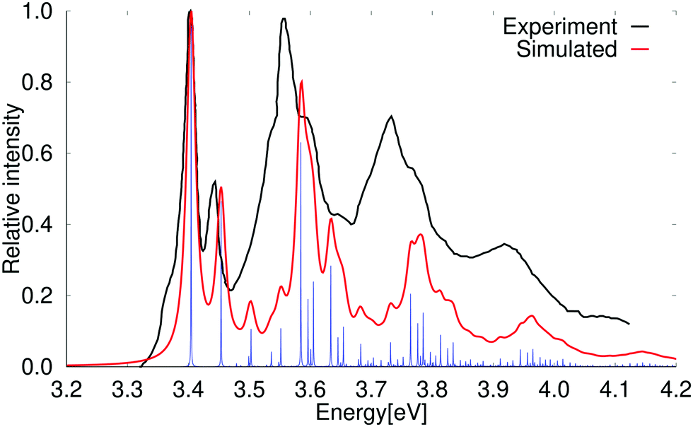Fig. 4 Comparison of the experimental and simulated spectra of the 1B_2u state of anthracene at the PBE0 level. The 0–0 transition energy of the simulated spectrum has been shifted by 0.49 eV. The experimental spectrum is taken from ref. 69. The red spectrum has been computed with lifetime (τ) of 72.6 fs; in the blue spectrum τ was set to 2420 fs.

The vibrational bands have been assigned in Table 5 by comparing the energy shifts with the vibrational energies of the vibrational states that belong to the total symmetric irreducible representation (A_g) of the D_2h point group. Comparison of the calculated and recorded spectra shows that the high-energy peaks of the calculated spectrum are blue shifted as compared to experiment probably due to the use of the harmonic approximation. The blue shift is larger at the high-energy part of the spectrum, because several slightly overestimated vibrational frequencies contribute to the shift. A similar DFT study has recent been performed at the generalized gradient approximation (GGA) level,⁷⁶ where they obtained a large red shift of the vertical excitation energy as compared to the experimental spectrum. All vibrational bands of the shifted spectrum were in good agreement with the experimental spectrum.⁷⁶ In a similar DFT study, Dierksen and Grimme obtained an absorption spectrum that also agreed well with the experimental one.³⁶ The high-energy vibrational bands were slightly red shifted relative to the experimental ones even though they employed the harmonic approximation that usually overestimates vibrational energies. The absorption spectrum calculated using a temperature of 423 K has a hot band below the 0–0 transition peak, which is seen as a shoulder on the low-energy side of the 0–0 band of the experimental spectrum.¹⁵ The hot band is missing in our simulated spectra, because in our calculations we assume a temperature of 0 K where only the lowest vibrational state of the electronic ground state is occupied.

Table 5 Assignment of the first few peaks of the absorption spectrum of anthracene calculated at PBE0 level. The vibrational bands originate from transitions involving the totally symmetric (A_g) vibrational modes of the 1B_2u excited state. The transition energies (in eV) and the vibrational shift of the transition energies (in cm⁻¹) are reported. The same numbering is used as in the ESI, whereas 14A_g is the first A_g mode, 27A_g is the third, 44A_g is the 5th, 53A_g is the 7th, 58A_g is the 8th, and 61A_g is the 9th A_g mode. All calculated vibrational energies are given in the ESI

Energy (in eV)	Shift (in cm^−1)	Rel. intensity	Assignment
3.402	0	1.000	0–0
3.451	396	0.463	14Ag
3.500	763	0.106	27Ag
3.549	1187	0.102	44Ag
3.582	1452	0.631	53Ag
3.593	1547	0.191	58Ag
3.602	1618	0.239	61Ag
3.631	1848	0.285	14Ag + 53Ag
3.643	1943	0.079	14Ag + 58Ag
3.651	2015	0.111	14Ag + 61Ag
3.680	2245	0.063	27Ag + 53Ag
3.729	2639	0.067	14Ag + 27Ag + 53Ag
3.762	2904	0.205	53Ag + 53Ag
3.773	2999	0.121	53Ag + 58Ag
3.782	3070	0.158	53Ag + 61Ag
3.810	3300	0.087	14Ag + 53Ag + 53Ag
3.831	3467	0.066	14Ag + 53Ag + 61Ag
3.962	4522	0.050	53Ag + 53Ag + 61Ag

---

Vibrational modes belonging to the A_g, B_1g and B_3g irreducible representations may contribute to the absorption spectrum of the 1B_2u state of anthracene. Only the A_g modes are active at the Franck–Condon level, whereas the B_1g modes may contribute at the Renner–Herzberg–Teller level via intensity borrowing from the strong ground-state transition of the 2B_3u state. Vibrational modes of the B_3g irreducible representation are expected to be less important, because the 1B_1u state is very high in energy.⁷⁷ Calculated and experimental values for the vibrational energies of the 1B_2u state are compared in Table 6. The calculated values for the low-energy A_g and B_1g modes agree well with the experimental ones, whereas the calculated values for high-energy modes differ significantly from the experimental ones.⁷⁷ Fewer vibrational modes are deduced from the experimental data rendering the comparison difficult. Since the high-energy vibrational peaks of the calculated absorption spectrum are generally blue shifted as compared to the experimental one, the vibrational mode corresponding to the calculated mode with an energy of 1282 cm⁻¹ is most likely missing in the experimental spectrum. The Renner–Herzberg–Teller effect does not play an important role for anthracene, since the main features of the calculated and measured absorption spectra agree. The lower-energy shoulder of the experimental spectrum is a hot band originating from the absorption of higher vibrational levels of the ground state.

Table 6 Comparison of calculated and measured vibrational energies (in cm⁻¹) of the 1B_2u state of anthracene. The experimental values are taken from ref. 77. The same mode numbering is used as in the ESI

Mode	E(Calc.)	E(Exp.)	Mode	E(Calc.)	E(Exp.)
14Ag	396	385	13B1g	238	232
21Ag	601	583	20B1g	453	473
27Ag	763	755	26B1g	511
40Ag	1061	1019	33B1g	728
44Ag	1187	1168	38B1g	919	889
47Ag	1282		41B1g	1098
53Ag	1452	1380	45B1g	1214	1184
58Ag	1547	1420	48B1g	1299
61Ag	1618	1501	52B1g	1418	1409
64Ag	3175		57B1g	1544	1514
68Ag	3189		59B1g	1583	1635
72Ag	3219

---

3.4 Simulation of the pentacene spectrum at the PBE0 level

The vertical excitation energy of the first excited state of pentacene is 1.95 eV (2.18 eV) at the PBE0 (BHLYP) level and has an oscillator strength of 0.040 (0.064). It belongs to the B_2u irreducible representation of the D_2h point group. The second excited state belonging to the B_3u irreducible representation has an oscillator strength of 0.004. The vertical excitation energy of the 1B_3u state calculated at the PBE0 level is 3.30 eV (3.48 eV).

At the second-order approximate coupled-cluster (CC2) level of theory, the calculated vertical excitation energy of the 1B_2u state is 2.34 eV with an oscillator strength of 0.057. The second excited state (1B_3u) has a vertical excitation energy of 3.29 eV and an oscillator strength of 0.003 at the CC2 level.

The absorption spectrum of pentacene has been recorded in rare gas matrices,⁷⁸ where significant vibrational transitions were reported at 85 cm⁻¹, 258 cm⁻¹, 1181 cm⁻¹, 1514 cm⁻¹, 2733 cm⁻¹, and 2991 cm⁻¹. The transitions can be assigned by comparing the vibrational energies with calculated ones. The vibrational transition at 85 cm⁻¹ most likely originates from the lowest B_1u mode.⁷⁹ The vibrational band at 258 cm⁻¹ corresponds to the lowest vibrational A_g mode, whose energy is calculated to 265 cm⁻¹. Since higher vibrational energies are blue shifted as compared to the experimental spectrum, an energy of 1226 cm⁻¹ is calculated for the band at 1181 cm⁻¹. The vibrational mode at 1184 cm⁻¹ also contributes to the peak. Several vibrational modes form the peak at 1514 cm⁻¹ in the experimental spectrum. The assignment of the high-energy part of the spectrum is difficult, because many combined vibrations contribute to the broad absorption band between 2.6 eV and 2.7 eV.

The absorption spectrum of the 1B_2u state of pentacene simulated at the PBE0 level is compared to the experimental one in Fig. 5.⁷⁸ A simulated absorption spectrum of pentacene obtained with a scaling factor of 0.95 is reported in the ESI.† The simulated spectrum shows that the first peaks in the experimental spectrum consist of one vibrational transition each, whereas the higher vibrational bands have significant contributions from several vibrational modes. The 0–0 transition energy of the simulated spectrum is 1.71 eV, which is 0.57 eV smaller than the experimental one. The assignment of the strongest vibrational contributions to the vibrational modes belonging to the total symmetric irreducible representation (A_g) of the D_2h point group is shown in Table 7. Three of the stronger bands are not assigned, because they are not due to any simple vibrational coupling with A_g modes. Comparison of the calculated and measured absorption spectra show that there are more peaks in the experimental spectrum than in the calculated one. The peak at the high-energy side of the 0–0 transition is 74 cm⁻¹ above the 0–0 transition, which can be compared to twice the vibrational energy of the first B_1u mode, whose energy is 39 cm⁻¹. Amirav, Even and Jortner⁷⁹ suggested that the low-energy butterfly mode belonging the B_1u irreducible representation leads to a fluorescence transition at about 77 cm⁻¹ below above the 0–0 peak, which is a plausible interpretation of the second peak that appears 74 cm⁻¹ above the 0–0 peak. Griffiths and Freedman had an alternative interpretation,⁸⁰ which is most likely incorrect judged from the present calculations. A closer inspection of the experimental absorption spectrum of pentacene in the Ne matrix shows that there is a weak transitions at about 346 cm⁻¹, which might also involve the lowest B_1u mode, since it is 81 cm⁻¹ above the vibrational transition corresponding to the first A_g mode.

Fig. 5 Comparison of the experimental and simulated spectra of the 1B_2u state of pentacene calculated at the PBE0 level. The 0–0 transition energy of the simulated spectrum has been shifted by 0.57 eV. The experimental spectrum is taken from ref. 78. The red spectrum has been computed with lifetime (τ) of 72.6 fs; in the blue spectrum τ was set to 2420 fs.

Table 7 Assignment of the first few peaks of the absorption spectrum of pentacene calculated at the PBE0 level. The vibrational bands originate from transitions involving the totally symmetric (A_g) vibrational modes of the 1B_2u excited state. The transition energies (in eV) and the vibrational shift of the transition energies (in cm⁻¹) are reported. The same numbering is used as in the ESI, whereas 15A_g is the first A_g mode, 39A_g is the 4th, 60A_g is the 6th, 64A_g is the 7th, 68A_g is the 8th, 75A_g is the 9th, 78A_g is the 10th, 81A_g is the 11th, 85 is the 12th, and 87A_g is the 13th A_g mode. All calculated vibrational energies are given in the ESI

Energy (in eV)	Shift (in cm^−1)	Rel. intensity	Assignment
2.286	0	1.000	0–0
2.319	265	0.245	15Ag
2.381	767	0.052	39Ag
2.433	1184	0.082	64Ag
2.438	1226	0.117	68Ag
2.462	1417	0.141	78Ag
2.467	1460	0.331	81Ag
2.479	1522	0.144	85Ag
2.484	1560	0.028	87Ag
2.494	1653	0.036
2.500	1680	0.076	15Ag + 78Ag
2.512	1787	0.034	15Ag + 85Ag
2.614	2621	0.041	60Ag + 87Ag
2.619	2662	0.039	60Ag + 90Ag
2.643	2855	0.044	75Ag + 85Ag
2.648	2896	0.056	75Ag + 87Ag
2.660	2992	0.049

---

The absorption spectrum of pentacene calculated at the GGA level has recently been reported.⁷⁶ They obtained a large red shift of the vertical excitation energy, whereas all vibrational bands of the shifted spectrum were in good agreement with the experimental spectrum, even though vibrational energies calculated in the harmonic approximation are generally overestimated.

3.5 Simulation of the pyrene spectrum at the PBE0 level

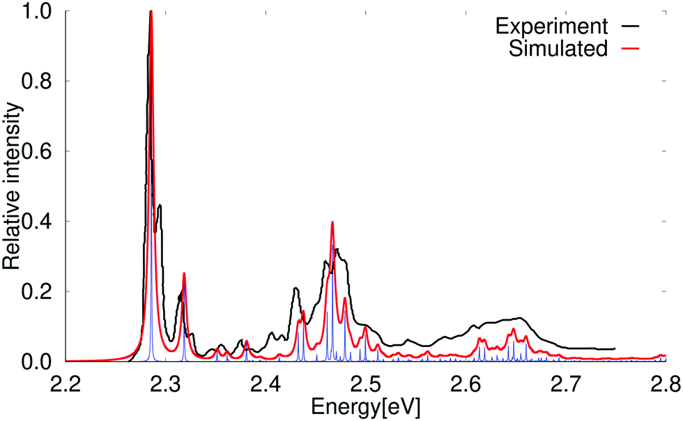
The vertical excitation energy of the first singlet excited state of pyrene is 3.78 eV (3.99 eV) at the PBE0 (BHLYP) level. The transition to the 1B_2u state has a relatively large oscillator strength of 0.272 (0.314). The calculated excitation energy of the other low-lying excited singlet state is 3.85 eV (4.07 eV). It belongs to the B_3u irreducible representation of the D_2h point group and has a very small oscillator strength.

At the CC2 level of theory, the two states appear in the reverse order, which is agreement with experiment. At the CC2 level, the vertical excitation energies of the 1B_2u and 1B_3u states are 4.07 eV and 3.78 eV, respectively. The B_2u has a large oscillator strength of 0.368 at the CC2 level, whereas for the B_3u state it is only 0.001. The experimental values for the excitation energy of the two states are 3.56 eV for the weak transition to the 1B_3u state and 3.82 eV for the strong transition to the B_2u state.^81,82

The experimental spectrum and simulated absorption spectrum calculated at the PBE0 level for the strong transition to the 1B_2u state are compared in Fig. 6. The two spectra agree well. A slightly better agreement is obtained when using a scaling factor of 0.90 as shown in the ESI.†

Fig. 6 Comparison of the experimental and simulated spectra of the 1B_2u state of pyrene. The 0–0 transition energy of the simulated spectrum has been shifted by 0.46 eV. The experimental spectrum is taken from ref. 69. The red spectrum has been computed with lifetime (τ) of 72.6 fs while in the blue spectrum τ was set to 2420 fs.

The higher vibrational bands of the calculated spectrum are slightly blue shifted as compared to the experimental spectrum, because the harmonic approximation generally yields too large vibrational energies. The vibrational bands were assigned by comparing the energies of the vibrational modes belonging to the total symmetric irreducible representation (A_g) of the D_2h point group. The assignment in Table 8 shows that the main contribution to the lowest vibrational bands originates mainly from one vibrational mode, whereas several modes contribute to the high-energy bands. Experimental and simulated absorption and emission spectra of pyrene have been previously reported by several research groups.^{36,64,69,74,76} Understanding the pyrene spectrum is of general interest, because the ratio between the intensities of the first and third vibrational band of the emission spectrum of pyrene is used for probing the dielectric constant of the environment of molecules in different contexts.^83–85

Table 8 Assignment of the first few peaks of the absorption spectrum of pyrene calculated at the PBE0 level. The vibrational bands originate from transitions involving the totally symmetric (A_g) vibrational modes of the 1B_2u excited state. The transition energies (in eV) and the vibrational shift of the transition energies (in cm⁻¹) are reported. The same numbering is used as in the ESI, whereas 14A_g is the first A_g mode, 31A_g is the third, 47A_g is the 5th, 52A_g is the 6th, 59A_g is the 8th, and 68A_g is the 10th A_g mode. All calculated vibrational energies are given in the ESI

Energy (in eV)	Shift (in cm^−1)	Rel. intensity	Assignment
3.842	0	1.000	0–0
3.894	411	0.288	14Ag
3.945	822	0.041	14Ag + 14Ag
3.985	1149	0.076	47Ag
3.999	1261	0.075	52Ag
4.021	1441	0.268	59Ag
4.046	1641	0.323	68Ag
4.072	1854	0.077	14Ag + 59Ag
4.097	2054	0.091	14Ag + 68Ag

---

4 Summary and conclusions

The absorption spectra of naphthalene, anthracene, pentacene and pyrene in the UV-Vis range have been calculated at the PBE0 and CC2 levels of theory using an efficient real-time generating function method. The vibrational coupling has been considered at the Franck–Condon level using the full Duschinsky formalism. We have neglected the Renner–Herzberg–Teller effect, which is less important for the lowest A_g → B_2u transition of these rigid molecules. The calculated absorption spectra agree well with available experimental data. We have considered only the electronic transition to the B_2u state, which is the lowest excited singlet state of anthracene and pentacene, whereas the weakly absorbing B_3u state is the lowest excited singlet state of naphthalene and pyrene. The electronic excitation energies are significantly underestimated at the PBE0 level, whereas the excitation energies calculated at the CC2 level are in better agreement with experimental data. The absorption spectra simulated at the PBE0 level agree well with the experimental ones when they are shifted by 0.48 eV, 0.49 eV, 0.57 eV and 0.46 eV for naphthalene, anthracene, pentacene and pyrene, respectively. At the CC2 level, the corresponding energy shift for naphthalene is 0.12 eV. Calculations employing simplified models such as the displaced harmonic oscillator approximation and the frequency-shifted displacement harmonic approximation models showed that they yield qualitatively the same spectra as obtained with the full Duschinsky treatment. Since the studied molecules are very rigid, the vibrational modes of the ground and excited states do not significantly differ. The individual vibrational peaks in the absorption spectra have been assigned by comparing the transition energies with vibrational energies of the A_g vibrational modes of the B_2u state. The peaks in the low-energy part of the spectra originate from single vibrational modes, whereas many vibrational modes contribute to the high-energy part of the absorption spectra rendering an accurate assignment difficult. The PBE0 and CC2 models generally tend to overestimate the harmonic vibrational frequencies leading to a blue shift of the high-energy part of the absorption spectra. We obtained a better overall agreement with experimental absorption spectra by using scaling factors of 0.90, 0.85, 0.95, 0.90 for naphthalene, anthracene, pentacene, and pyrene, respectively. Even though we were not able to find any universal scaling factor for the vibrational frequencies, we found that scaling factors smaller than one improve the agreement with the experimental spectra.

Conflicts of interest

There are no conflicts to declare.

Acknowledgements

This research has been supported by the Academy of Finland through projects (275845, 287791 and 314821 and the MESIOS project 277579). CSC – the Finnish IT Center for Science and the Finnish Grid and Cloud Infrastructure (persistent identifier urn:nbn:fi:research-infras-2016072533) are acknowledged for computer time.

Notes and references

1. E. Stendardo, F. Avila Ferrer, F. Santoro and R. Improta, J. Chem. Theory Comput., 2012, 8, 4483–4493.
2. J. Bloino, A. Baiardi and M. Biczysko, Int. J. Quantum Chem., 2016, 116, 1543–1574.
3. F. Santoro and D. Jacquemin, Wiley Interdiscip. Rev.: Comput. Mol. Sci., 2016, 6, 460–486.
4. E. Tapavicza, F. Furche and D. Sundholm, J. Chem. Theory Comput., 2016, 12, 5058–5066.
5. E. Brunk and U. Röthlisberger, Chem. Rev., 2015, 115, 6217–6263.
6. E. Tapavicza, G. D. Bellchambers, J. C. Vincent and F. Furche, Phys. Chem. Chem. Phys., 2013, 15, 18336–18348.
7. I. Tavernelli, U. F. Röhrig and U. Rothlisberger, Mol. Phys., 2005, 103, 963–981.
8. C.-M. Suomivuori, A. P. Gamiz-Hernandez, D. Sundholm and V. R. I. Kaila, Proc. Natl. Acad. Sci. U. S. A., 2017, 114, 7043–7048.
9. C. Cisneros, T. Thompson, N. Baluyot, A. C. Smith and E. Tapavicza, Phys. Chem. Chem. Phys., 2017, 19, 5763–5777.
10. T. Thompson and E. Tapavicza, J. Phys. Chem. Lett., 2018, 9, 4758–4764.
11. E. Tapavicza, T. Thompson, K. Redd and D. Kim, Phys. Chem. Chem. Phys., 2018, 20, 24807–24820.
12. S. Mukamel, S. Abe and R. Islampour, J. Phys. Chem., 1985, 89, 201–204.
13. Y. J. Yan and S. Mukamel, J. Chem. Phys., 1986, 85, 5908–5923.
14. F. Santoro, A. Lami, R. Improta, J. Bloino and V. Barone, J. Chem. Phys., 2008, 128, 224311.
15. Y. Niu, Q. Peng, C. Deng, X. Gao and Z. Shuai, J. Phys. Chem. A, 2010, 114, 7817–7831.
16. H. Ma, J. Liu and W. Liang, J. Chem. Theory Comput., 2012, 8, 4474–4482.
17. H.-C. Jankowiaka, J. L. Stuber and R. Berger, J. Chem. Phys., 2007, 127, 234101.
18. J. Huh and R. Berger, J. Phys.: Conf. Ser., 2012, 380, 012019.
19. M. Etinski, J. Tatchen and C. M. Marian, J. Chem. Phys., 2011, 134, 154105.
20. M. Etinski, V. Rai-Constapel and C. M. Marian, J. Chem. Phys., 2014, 140, 114104.
21. M. Etinski, M. Petković, M. M. Ristić and C. M. Marian, J. Phys. Chem. B, 2015, 119, 10156–10169.
22. M. P. Kabir, Y. Orozco-Gonzalez and S. Gozem, Phys. Chem. Chem. Phys., 2019, 21, 16526–16537.
23. T. R. Faulkner and F. S. Richardson, J. Chem. Phys., 1979, 70, 1201–1213.
24. F. Duschinsky, Acta Physicochim. URSS, 1937, 7, 551–566.
25. A. M. Mebel, M. Hayashi, K. K. Liang and S. H. Lin, J. Phys. Chem. A, 1999, 103, 10674–10690.
26. F. Metz, M. Robey, E. Schlag and F. Dörr, Chem. Phys. Letters, 1977, 51, 8–12.
27. A. Baiardi, J. Bloino and V. Barone, J. Chem. Theory Comput., 2013, 9, 4097–4115.
28. R. Renner, Z. Phys., 1934, 92, 172–193.
29. G. Herzberg and E. Teller, Z. Phys. Chem., Abt. B, 1933, 21, 410–446.
30. G. Atkinson and C. Parmenter, J. Mol. Struct., 1978, 73, 52–95.
31. A. Bacon, J. Hollas and T. Ridley, Can. J. Phys., 1984, 62, 1254–1263.
32. L. A. Bizimana, W. P. Carbery, T. A. Gellen and D. B. Turner, J. Chem. Phys., 2017, 146, 084311.
33. G. Orlandi and W. Siebrand, J. Chem. Phys., 1973, 58, 4513–4523.
34. G. J. Small, J. Chem. Phys., 1971, 54, 3300–3306.
35. H. Fliegl and D. Sundholm, Phys. Chem. Chem. Phys., 2014, 16, 9859–9865.
36. M. Dierksen and S. Grimme, J. Chem. Phys., 2004, 120, 3544–3554.
37. N. O. C. Winter, N. K. Graf, S. Leutwyler and C. Hättig, Phys. Chem. Chem. Phys., 2013, 15, 6623–6630.
38. A. S. Coolidge, H. M. James and R. D. Present, J. Chem. Phys., 1936, 4, 193–211.
39. T. Sharp and H. Rosenstock, J. Chem. Phys., 1964, 41, 3453–3463.
40. W. Siebrand, J. Chem. Phys., 1967, 46, 440–447.
41. J. P. Perdew, K. Burke and M. Ernzerhof, J. Chem. Phys., 1996, 105, 9982–9985.
42. F. Weigend and R. Ahlrichs, Phys. Chem. Chem. Phys., 2005, 7, 3297–3305.
43. S. Grimme, J. Antony, S. Ehrlich and H. Krieg, J. Chem. Phys., 2010, 132, 154104.
44. P. Deglmann and F. Furche, Chem. Phys. Letters, 2002, 362, 511–518.
45. R. Ahlrichs, M. Bär, M. Häser, H. Horn and C. Kölmel, Chem. Phys. Letters, 1989, 162, 165–169.
46. F. Furche, R. Ahlrichs, C. Hättig, W. Klopper, M. Sierka and F. Weigend, Wiley Interdiscip. Rev.: Comput. Mol. Sci., 2014, 4, 91–100.
47. TURBOMOLE V7.3 2018, a development of University of Karlsruhe and Forschungszentrum Karlsruhe GmbH, 1989–2007, TURBOMOLE GmbH, since 2007; available from http://www.turbomole.com.
48. C. Møller and M. S. Plesset, Phys. Rev., 1934, 46, 618–622.
49. W. Humphrey, A. Dalke and K. Schulten, J. Mol. Graphics, 1996, 14, 33–38.
50. R. Bauernschmitt and R. Ahlrichs, Chem. Phys. Letters, 1996, 256, 454–464.
51. F. Furche and R. Ahlrichs, J. Chem. Phys., 2002, 117, 7433–7447.
52. M. E. Casida and M. Huix-Rotllant, Annu. Rev. Phys. Chem., 2012, 63, 287–323.
53. M. E. Casida, in Recent Advances in Density Functional Methods, Part I, ed. D. P. Chong, World Scientific, Singapore, 1995, p. 155.
54. E. Runge and E. K. U. Gross, Phys. Rev. Lett., 1984, 52, 997–1000.
55. A. D. Becke, J. Chem. Phys., 1993, 98, 1372–1377.
56. O. Christiansen, H. Koch and P. Jørgensen, Chem. Phys. Letters, 1995, 243, 409–418.
57. J. Schirmer, Phys. Rev. A: At., Mol., Opt. Phys., 1982, 26, 2395–2416.
58. C. Hättig and F. Weigend, J. Chem. Phys., 2000, 113, 5154–5161.
59. A. Köhn and C. Hättig, J. Chem. Phys., 2003, 119, 5021–5036.
60. C. Hättig, Adv. Quantum Chem., 2005, 50, 37–60.
61. G. A. George and G. C. Morris, J. Mol. Spectrosc., 1968, 26, 67–71.
62. G. Herzberg, Electronic spectra and electronic structure of polyatomic molecules, Van Nostrad Reinhold, New York, 1966.
63. J. G. Angus and G. C. Morris, Mol. Cryst. Liq. Cryst., 1970, 11, 257–277.
64. A. Y. Freidzon, R. R. Valiev and A. A. Berezhony, RSC Adv., 2014, 4, 42054–42065.
65. W. Domcke, D. Yarkony and H. Köppel, Conical intersections: electronic structure, dynamics & spectroscopy, World Scientific, 2004.
66. F. G. Mehler, J. Reine Angew. Math., 1866, 66, 161–176.
67. M. Krykunov, S. Grimme and T. Ziegler, J. Chem. Theory Comput., 2012, 8, 4434–4440.
68. A. Bree and T. Thirunamachandran, Mol. Phys., 1962, 5, 397–405.
69. J. Ferguson, L. W. Reeves and W. G. Schneider, Can. J. Chem., 1957, 35, 1117–1136.
70. J. P. Merrick, D. Moran and L. Radom, J. Phys. Chem. A, 2007, 111, 11683–11700.
71. M. Suto, X. Wang, J. Shan and L. C. Lee, J. Quant. Spectrosc. Radiat. Transfer., 1992, 48, 79–89.
72. H. Grosch, Z. Sárossy, H. Egsgaard and A. Fateev, J. Quant. Spectrosc. Radiat. Transfer, 2015, 156, 17–23.
73. L. E. Lyons and G. C. Morris, J. Chem. Soc., 1959, 1551–1558.
74. A. Thöny and M. J. Rossi, J. Photochem. Photobiol., A, 1997, 104, 25–33.
75. A. Bree and L. E. Lyons, J. Chem. Soc., 1956, 2662–2670.
76. R. Rüger, T. Niehaus, E. van Lenthe, T. Heine and L. Visscher, J. Chem. Phys., 2016, 145, 184102.
77. W. R. Lambert, P. M. Felker, J. A. Syage and A. H. Zewail, J. Chem. Phys., 1984, 81, 2195–2208.
78. T. M. Halasinski, D. M. Hudgins, F. Salama, L. J. Allamandola and T. Bally, J. Phys. Chem. A, 2000, 104, 7484–7491.
79. A. Amirav, U. Even and J. Jortner, Chem. Phys. Letters, 1980, 72, 21–24.
80. A. M. Griffiths and P. A. Freedman, J. Chem. Soc., Faraday Trans. 2, 1982, 78, 391–398.
81. J. B. Briks, Photophysics of Aromatic Molecules, Wiley, New York, 1970.
82. Y. L. Wang and G. S. Wu, Int. J. Quantum Chem., 2008, 108, 430–439.
83. V. Glushko, M. Thaler and C. Karp, Arch. Biochem. Biophys., 1981, 210, 33–42.
84. M. D'Abramo, M. Aschi and A. Amadei, Chem. Phys. Lett., 2015, 639, 17–22.
85. K. W. Street and W. E. Acree, Appl. Spectrosc., 1988, 42, 1315–1318.

---

Footnote

† Electronic supplementary information (ESI) available: The Cartesian coordinates of the optimized molecular structures and the calculated harmonic frequencies of the studied molecules. The scaled absorption spectra. The absorption spectra for anthracene calculated with and without Duschinsky rotation are compared. See DOI: 10.1039/c9cp04178h

---