Molecular dynamics involving proton exchange of a protic ionic liquid–water mixture studied by NMR spectroscopy

Abstract

Protic ionic liquids (PILs) are proposed as alternative anhydrous proton conducting electrolytes for intermediate temperature fuel cells. One of the key factors in their performance as electrolytes, as far as charge transport is concerned, is their proton conductivity. Noting the success of water-containing electrolytes and recognising faster proton mobility than structural relaxation (via mechanisms such as Grotthuss) as their advantage, such an advantage is envisaged for PILs and in some cases deduced. As extended hydrogen bond networks and proton exchange are at the heart of these mechanisms, here we report our results on a prototypical characterisation of proton exchange in a PIL (C₂HimNTf₂)–water mixture. NMR lineshape analysis and exchange spectroscopy (EXSY) are used to quantify the proton exchange rate. The obtained exchange rate is then used to explain the diffusion behaviour of the exchangeable proton as measured by pulse field gradient NMR methods; a marginal anomaly in the translational dynamics of the exchangeable proton in the form of a faster NH proton is observed. As far as we know this is the first report on systematic characterisation of proton exchange in PILs with the aim of understanding its effect on translational motion as a way of discerning exchange related mobility anomalies.

---

1 Introduction

Ionic liquids (ILs) as a class of material are regarded as alternative electrolytes for electrochemical devices.^1–6 A subclass of them, branded protic ionic liquids (PILs), are proposed as proton conducting electrolytes by virtue of having protons labile to reduction, and as alternatives to hydrated Nafion by virtue of their lower volatility.²

As far as proton conduction is concerned, the most successful fuel cell electrolytes share the property of showing proton mobilities higher than those of the proton carriers through generally accepted mechanisms involving hydrogen bond formation–dissociation i.e. proton exchange. Theodor von Grotthuss is credited with having proposed for the first time such a mechanism for ionic conduction in liquid water, being composed of oppositely charged “bodies” which carry charge in opposite directions by successive dissociation.⁷ Different interpretations of this “Grotthuss mechanism” in its modern form are presented, supported by/confronted with experimental results, and reviewed in the literature.^8–10 All of these closely related yet different mechanisms have something in common and that is the presence of hydrogen bonds and the exchange of protons through them. It is this proton exchange process and its effect on the measured proton mobility that are the subject of this study.

It is, therefore, not surprising that toward the success of PILs as fuel cell electrolytes, the existence of Grotthuss type proton transport in materials is envisioned, sought, and reported.^11–13 Other than nuclear magnetic resonance (NMR) spectroscopy results, discussed below, notable experimental evidence is reported for imidazoliumNTf₂–imidazole, ImHNTf₂–Im, mixtures using quasielastic neutron scattering (QENS)¹¹ and for C₁HimOAc using Raman spectroscopy.¹² The latter case of C₁HimOAc was recently picked up for an ab initio molecular dynamics study of its proton transport mechanism,¹³ rationalising the experimental results by demonstrating instances of proton transport through acetic acid wires, yet ruling out proton hopping/tunnelling.‡

The majority of the reported experimental evidence for proton transport “anomalies”, explained below, in PILs come from self-diffusion coefficient measurements of hydrogen atoms (and to a lesser extent fluorine atoms) using pulse field gradient (PFG) NMR spectroscopy routines. Anomalies§ are reported in some cases where the measurements yield a higher self-diffusion coefficient for the exchangeable proton than other species in the system. It is convincing evidence of the presence of translational mobility paths available only to the exchangeable proton, provided that the susceptibility of the methods to interferences (e.g. impurities like water) is carefully considered.^14,15 It should be noted that, even in “normal” cases, proton exchange complicates the interpretation of diffusion results as here the diffusion behaviour is not of a single species but of all accessible to the proton during the observation time. These complications, when neglected, for example in the case of a water impurity, can cause an overestimation of the proton diffusion coefficient. The complications can to some extent be avoided by choosing experimental parameters such that they become negligible,¹⁴ however, when they are intrinsic to the phenomenon under study i.e. Grotthuss-like mechanisms, a quantitative account of their effects is necessary. Here, we present the results of our efforts in understanding and explaining the effect of proton exchange on self-diffusion behaviour after quantifying proton exchange rates using various NMR techniques.

Dynamic NMR spectroscopy is almost as old as the technique itself^16,17 and its application in the study of chemical exchange well presented.¹⁸ The effect of exchange on self-diffusion coefficient measurements using PFG methods is also discussed in the literature¹⁹ and will be discussed in greater detail in Section 3. Proton exchange rate determination using dynamic NMR techniques is seen in reports relevant to this study where exchange spectroscopy (EXSY) is used to measure the exchange rate of imidazole ring protons in the aprotic ionic liquid 1-ethyl-3-methylimidazolium acetate, C₁C₂imOAc.²⁰ In a more recent study, lineshape analysis is used to determine proton exchange rates between water and a polymerised PIL in their dimethylsulfoxide (DMSO) solution.²¹ The effects of exchange on signal attenuation curves resulting from PFG studies in similar systems are sometimes mentioned but have never been quantitatively accounted for.

In this study, we use NMR spectroscopy to characterise proton exchange in a PIL (1-ethylimidazolium bistriflimide, C₂HimNTf₂)–water mixture. Lineshape analysis is used to measure the exchange rate and its temperature dependance is analysed to estimate the exchange activation energy. EXSY is also used to successfully reproduce the measured rate. The effect of exchange on signal attenuation curves from PFG measurements is shown and rationalised using the measured rate. It is shown that the effect is adequately described by the Kärger^22,23 equation.

2 Experimental methods

Ethylimidazolium bistriflimide, C₂HimNTf₂, was purchased from Iolitech (Lot# P00170.1.2-IL-0269), stored under an inert atmosphere and used with no further purification. The water content was measured using Karl–Fischer titration to be 1089 ppm. Deuterium oxide (D₂O 99.9 atom% D) was purchased from Sigma-Aldrich and used as received. The two liquids were mixed to yield a water mole fraction of 0.33 ± 0.01. The mixture was also sealed in a vial and heated at 70 °C for 20 minutes to achieve complete mixing. Around 500 μL of the mixture was transferred into a 5 mm NMR tube and the tube was sealed.

An AVANCE III HD Bruker NMR spectrometer with a magnetic field of 14.1 T and a basic transmitter frequency of 600.130 MHz and a 5 mm diff30 probe with a water-cooled gradient coil was used for NMR characterisation of the sample. The temperature of the probe was controlled with a stream of nitrogen gas and the temperature sensor calibrated with methanol/ethylene glycol routinely. For PFG experiments done at 298 K, the temperature of the water bath (gradient coil) was kept at 293 K. After inserting the sample in the probe, 20 minutes of temperature equilibration, careful tuning/matching of the probe, shimming of the magnetic field, pulse calibration, and T₁/T₂ measurements, a proton spectrum was collected with 8 transients and a recycle delay of 15 seconds according to the largest longitudinal relaxation time. The chemical shifts were referenced externally to tetramethylsilane (TMS) using the residual water peak in D₂O before each experiment. Data processing was done using Topspin 3.5 and further Python 3.6. Mnova 10.0.0 software was used to prepare the 2D spectrum. These one-dimensional spectra were used for integration and lineshape analysis of the peaks.

2D EXSY (phase sensitive 2D NOESY, using the noesygpphpp sequence in Topspin) spectra with 1 ms gradient pulses during the mixing time and purge pulses before a relaxation delay of 17 seconds were collected while the mixing time was changed from 3 to 200 ms, as described in the text. Each spectrum was processed to obtain the peak integrals used in calculating the proton exchange rate.

A PFG-stimulated echo pulse sequence with bipolar gradients²⁴ was used for diffusion experiments. Longitudinal eddy current delay (LED) proved unnecessary with bipolar gradients and was not used. With 16 transients recorded after 15 seconds of relaxation delay, a diffusion time between 25 and 1000 ms, and a gradient pulse duration of 2 ms, the magnetic field gradient was increased accordingly to obtain an attenuation of signals of 6 orders of magnitude.

3 Results and discussion

For simplicity, a 2 : 1 mixture of PIL : D₂O (χ_water = 0.33) was chosen to give a 1 to 1 ratio of imidazolium NH to water OH to obtain a system with a symmetrical two site exchange reaction. It is assumed that the residence time of the exchangeable proton on the anion is insignificant due to the anion's low basicity, which is a reasonable assumption given a Hammett acidity function (H₀) value of −19 for its conjugate acid.²⁵ A summary of the results is presented in Table 1.

Table 1 A summary of the proton exchange rate measurement results

Property	Quantity (unit)
k ^298ex(lineshape)	19–35 (s^−1)
k ^298ex(EXSY)	19 ± 1 (s^−1)
E a of proton transfer	58 ± 1 (kJ mol^−1)

---

The 1D proton NMR spectrum of the mixture at 298 K along with the chemical structure and peak assignment is shown in Fig. 1. The presence of separate OH and NH peaks shows that the exchange is slower than the NMR time scale (<5200 Hz). The integration of the peaks confirms the correct stoichiometry and complete isotope scrambling within 5%. The exchangeable proton signals are broader than the non-exchangeable ones indicating that the process is in the slow–intermediate regime. The additional broadness of the NH signal is due to ¹⁴N coupling; to avoid complication, therefore, the OH signal is picked for lineshape analysis.

Fig. 1 ¹H NMR spectrum of the C₂HimNTf₂–water mixture at 298 K. The OH (at 3.59 ppm) and NH (at 12.24 ppm) peaks are integrated (over 3 times their fwhm) to show the stoichiometry of the mixture (χ_water = 0.33) and complete isotope scrambling. The inset is the water peak magnified (red solid line) and fitted with a Lorentzian function around its maximum (black dashed line). The fit gives a full width at half maximum (fwhm) of 11 Hz, which corresponds to an exchange rate of 35 s⁻¹ if the linewidth is considered to be solely from exchange. An exchange rate of 19 s⁻¹ is obtained if a contribution of 5 Hz (based on the fwhm of non-exchangeable protons) is subtracted as a result of all other broadening phenomena.

The NMR lineshape in the case of an uncoupled spin system in intermolecular exchange is adequately described by Bloch equations modified by including a pseudo-first order decay term; a thorough treatment can be found in any text on dynamic NMR spectroscopy.^16,17 By estimating T^eff₂ in the absence of exchange from non-exchanging proton signals, the pseudo-first order rate constant (k) can be calculated from the width (full width at half maximum, fwhm) of the signal according to eqn (1). The inset in Fig. 1 shows the OH signal fitted to a Lorentzian shape to obtain a fwhm of 11 Hz, while the non-exchanging aromatic CH signals have widths of 5 Hz (corresponding to a T^eff₂ of 1/5π). Eqn (1) gives a reasonable value for the rate constant between 19 s⁻¹ (if we consider T^eff₂) and 35 s⁻¹ (if we take all the 11 Hz to be a result of exchange). The smaller value is likely to be closer to the true value.

As the temperature is raised, the linewidths of exchangeable protons increase, which is expected from an increase in the exchange rate at higher temperatures. Fig. 2 shows the effect of temperature (T) on the linewidth of the OH signal. The inset plot is of the linewidths of different representative signals against temperature showing that the exchanging signals get broader with temperature while the non-exchanging signal's lineshape remains unchanged. The exponential looking change in the linewidth of the exchangeable signals can be fitted to the Arrhenius equation, eqn (2), as shown in Fig. 3 to extract an activation energy (E_a) for the exchange process. A value of 58.3 ± 0.9 kJ mol⁻¹ is obtained.

Fig. 2 The effect of temperature on the proton exchange rate as reflected in the OH peak linewidth. The inset is a plot of linewidths versus temperature for the two exchanging signals (NH and OH) and one non-exchanging (C²H), resembling a rate process described by an activation energy (E_a) and governed by the Arrhenius equation (eqn (2), see also Fig. 3). The error bars on the fitted linewidths are smaller than the symbol sizes.

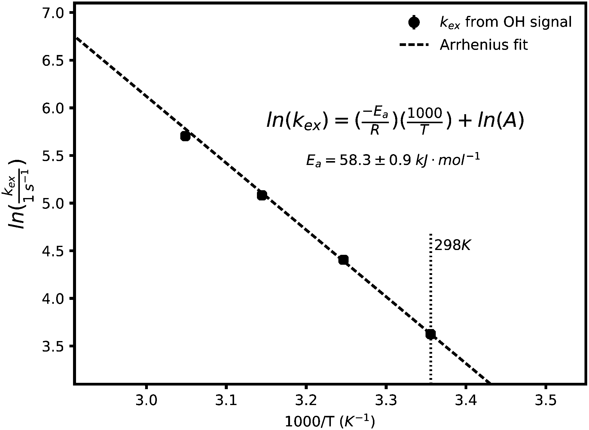Fig. 3 Arrhenius fit of the proton exchange rates at different temperatures obtained from lineshape analysis of the OH signal. An activation energy of 58.3 ± 0.9 kJ mol⁻¹ is obtained, to be compared with 10 kJ mol⁻¹ for water. The uncertainty in the fitted slope is set to one standard deviation.

In this equation A is a constant and R the universal gas constant. The activation energy can be compared with the approximate value of 10 kJ mol⁻¹ for the energy barrier of proton hopping in water,²⁶ suggesting a lower likelihood of fast/decoupled proton mobility.

The proton exchange in this case is slow enough, and the protons' relaxation times are long enough, to be studied by measuring the exchange of longitudinal magnetisation. This is done by using a two dimensional homonuclear experiment (2D-EXSY) resulting in cross peaks caused by magnetisation transfer between the exchanging sites during a mixing time τ_m. A typical 2D spectrum is included in the accompanying ESI† document. Derivation of the theoretical peak intensities as function of the mixing time can be found²⁷ to follow eqn (3) when the spin–lattice relaxation times for the exchanging spins are the same:

where I_cross and I_diag are cross and diagonal peak intensities, and sin h, cos h, and tan h are corresponding hyperbolic functions. Fig. 4 shows how the cross to diagonal peak intensity ratios obtained at 298 K change with changing the mixing time from 3 to 200 ms. A rate of 19 s⁻¹ is obtained, consistent with the lineshape analysis results. It should be noted that the 2D EXSY and 2D NOESY pulse sequences are identical and the experiments equivalent. As a result, the spectrum contains, in general terms, cross peaks from cross relaxation due to both chemical exchange and the nuclear Overhauser effect (NOE). In a phase sensitive spectrum the two effects have opposite signs, yet if present in a single pair of cross peaks, they cannot be told apart. The intermolecular NOE effect between the exchanging protons is deemed negligible here (by comparison to the (lack of) pure intramolecular NOE between the non-exchanging protons) in the presence of a much more efficient path of (relatively fast) chemical exchange. The argument is presented in the ESI† document.

Fig. 4 Cross to diagonal peaks ratio obtained from 2D-EXSY spectra of a C₂HimNTf₂–water mixture at 298 K for mixing times between 3 and 200 ms. The full curve fit and the initial linear fit give a proton exchange rate of 19 s⁻¹ consistent with the value obtained from lineshape analysis. Uncertainties in the fitted parameters are set to one standard deviation. The error bars on the integral ratios are smaller than the symbol sizes.

With a satisfactory estimate of the proton's exchange rate, we now focus our attention on the study of its translational motion through measuring its self-diffusion coefficient. PFG-stimulated echo (STE)^28–30 was used as described in Section 2. It works out that the measured echo amplitude follows eqn (4):

I = I₀e^{−(γδg)2D(Δ−δ/3)} (4)

where I is the signal intensity, I₀ is the signal intensity of the echo at zero gradient, g is the gradient strength, D is the self-diffusion coefficient, δ is the length of the gradient pulse, and Δ is the diffusion time. The self-diffusion coefficient can be obtained by taking the slope of the signal attenuation's natural logarithm versus (γδg)²(Δ − δ/3), abbreviated as b, known as a Stejskal–Tanner (ST) plot.

Fig. 5 shows such plots for a non-exchanging aromatic proton. The experiment was done with different diffusion times to show the same linearity over 6 orders of magnitude signal attenuation and gave a self-diffusion coefficient of 3.14 ± 0.06 × 10⁻¹¹ m² s⁻¹, indicating no interference from convection, restricted diffusion, or chemical exchange. The differences in the lines' intercepts are due to increasing signal loss to longitudinal relaxation as the diffusion time, Δ, is increased.

Fig. 5 Stejskal–Tanner plot for a non-exchanging proton (aromatic C²H on the imidazole ring) of a C₂HimNTf₂–water mixture at 298 K showing the same mono-exponential behaviour for different diffusion times over 6 orders of magnitude, manifesting the absence of exchange or convection. The dashed lines are linear fits to the data. The error bars are smaller than the symbol sizes. b is (γδg)²(Δ − δ/3).

It has been observed from the early stages that chemical exchange accompanies diffusion in affecting echo amplitudes, as is also observed in the liquid mixture investigated here, see Fig. 6. Its effect has been discussed in the literature^19,22,23 and a simple treatment of how it affects the magnetisation dynamics of the exchanging spins (M_i and M_j) is shown in eqn (5):

Here t refers to the diffusion time and k_i is the inverse of the spin's residence time in state i (k_i = 1/τ_i). The equations are solved for the boundary conditions M_i(t = 0) = M_i,0 (and M_j(t = 0) = M_j,0) in the slow exchange regime to give the observable magnetisation as a function of the gradient pulse area, diffusion coefficients, exchange rates, and diffusion time;²³ to see the solutions please look at the ESI† document.

Fig. 6 Attenuation of an exchanging signal deviates from a mono-exponential behaviour due to exchange during the diffusion time. The behaviour, in the simple case of a symmetrical two site exchange, is governed by the exchange rate and the diffusion coefficients of the two species. The dashed lines are linear fits to get the initial slopes. The error bars are smaller than the symbol sizes.

To quantify the effect of exchange on the ST plots of exchanging signals, we focused our attention on the initial slope and its change as Δ is varied. The initial slopes for three different signals (NH, OH, and C²H) with different diffusion times are presented in Fig. 7; a clear trend is seen.

Fig. 7 The effect of changing diffusion time on the initial slopes of exchanging signals' attenuations. Note that increasing diffusion time does not affect the non-exchanging C²H signal whereas it increases the attenuation rate of the slower (NH) signal by mixing with a faster decaying (OH) signal and vice versa. The dashed lines are simulated based on the solution of eqn (5) with input parameters from experimental results.

As shown in Fig. 5, the ST slope of a non-exchanging signal is independent of Δ while the initial slopes for the exchanging protons' ST plots change monotonically according to the self-diffusion coefficients of each site in the absence of exchange and the residence time of the proton in each state (here, a symmetrical two site exchange case, τ_NH = τ_OH). Water (OH) is reasonably assumed to be more quickly diffusing than the cation (NH) in this system. As more time is given for the two states to exchange, by increasing Δ, the slower species shows faster dynamics and vice versa.

An attempt to fit all the data globally to the solution of eqn (5) (eqn (S2) in the ESI† document) using a single set of parameters failed despite using elaborate fitting algorithms. The signal attenuation was then simulated using eqn (S2) using carefully measured parameters such as longitudinal and transverse relaxation times, integrals, diffusion coefficients, and exchange rates for each signal. An exchange rate of 19 s⁻¹ for exchanging and 0 s⁻¹ for non-exchanging protons was used. As for the self-diffusion coefficients of NH in the absence of exchange, the same value as for non-exchanging signals was used. The self-diffusion coefficient of OH (water) in the absence of exchange in this exact system cannot be measured so a value of 1.55 × 10⁻¹⁰ m² s⁻¹, which gave the closest simulation output to experimental results, was used. Representative simulation outputs are shown in Fig. S3 in the ESI† document and show good agreement with the initial part of each experimental ST curve but weak agreement with the tail part. A brief explanation about the possible reasons for the models inapplicability/insufficiency is given in the ESI† document. As a result, we focused our attention on the initial slope of the ST curves since the experimental results are thought to be more reliable (due to higher signal intensity) and also the model is more successful in simulating the initial slopes. The results of simulation of the initial slopes for the three signals in Fig. 7 are shown as dashed lines. In general, good agreement between the simulated and experimental results is seen. This is interesting in the sense that often faster dynamics of exchangeable protons can be explained through careful treatment of the exchange effect. It also shows to what extent a simple model such as eqn (5) can be used for this purpose. The NH proton seems to show marginally faster dynamics than what eqn (5) predicts, yet is not considered significant in our opinion. This means that the self-diffusion behaviour of this PIL–water mixture as measured by NMR diffusometry can be explained without the need to resort to anomalous mobility mechanisms.

A discussion of proton transport in PILs seems timely in the light of reported results. Where charge transport properties are discussed, strong–weak classification of electrolytes can also be applied to PILs based on the degree of ionisation, α.³¹ A high degree of ionisation corresponds to a higher concentration of ionic species, whereas a low α indicates the presence of neutral species. Whether to get a high or low α depends on the affinity of the anion for the labile proton(s) of the cation and is ultimately determined by the anion's hydrogen bond basicity.^25,32,33

Intuitively, to achieve higher conductivities desirable for electrochemical applications, higher degrees of ionisation are tried. It can be achieved by using anions of increasingly lower basicity, the conjugate bases of superacids, resulting in firm attachment of the exchangeable proton to the cation for the lack of any other accepting site. An example can be found in the first author's PhD dissertation,³² page 142, where a proton NMR spectrum of diethylmethylammonium tetrachloroaluminate, N₂₂₁HAlCl₄, shows well-resolved ¹⁵N splitting of the exchangeable proton, showing the proton does not appear exchangeable anymore. This “big hammer” approach succeeds in making PILs with properties matching those of their aprotic counterparts, some desirable such as low vapour pressure, yet counters their benefits too as the liquid tends to form quasi-lattice structures with the increased Coulomb interactions. PILs made this way would at best show conductivities/transport numbers similar to aprotic ILs, limiting the proton mobility to that of the cation when we know the proton, as the smallest ion, has the potential for higher/selective mobility.

To unlock the proton's potential for exceptional mobility, it needs to be liberated from the bound state and be given the possibility to exchange.³⁴ One possible way is by choosing the anion to have a higher hydrogen bond basicity such that it can accept the exchangeable proton from the cation. This neutralisation process means fewer ions and a lower degree of ionisation, which seems counter-intuitive and might indeed be a trade-off. An example is C₁HimOAc, for which a degree of ionisation lower than 0.33 (as low as 0.17 or even 0.01 based on the method), yet an unexpected ionic conductivity, is reported and attributed to the Grotthuss mechanism.^12,13 Here, the proton mobility has come at the expense of lower α and higher volatility. Another approach is the addition of a component to a fully ionic PIL in order to perturb the structure of the IL and provide proton exchange sites. ImHNTf₂ is an example PIL with a high degree of ionisation and is reported¹¹ to show proton mobility decoupled from the motion of bigger species in the mix when mixed with excess base. In ImHNTf₂, the low basicity NTf₂⁻ anion has such a low affinity for protons that the protons are stuck on the cations with nowhere to go. The addition of excess base, Im, provides hydrogen bond acceptor sites and makes exchange and decoupled mobility possible. Even though not reported in this specific study, addition of excess acid can also have a similar effect by providing hydrogen bond donor sites, of the added acid, with such high activities for which the anion would show affinity.³⁵ Depending on the nature of the component added, this second approach presents challenges as well. Addition of excess acid can also make the mixture corrosive and unfavourable. The volatility of the added component is also a disadvantage. As such, the addition of a suitable, non-volatile (maybe polymeric, similar to the polymer-in-salt concept³⁶) component seems to be an approach likely to succeed; it is the subject of ongoing research.

Water, as an amphoteric molecule, can be both a hydrogen bond donor and an acceptor.³⁷ Even though volatile, its inevitable presence especially in fuel cells makes its consideration worthwhile. It is not unreasonable to study its addition to PILs with large α in order to promote proton exchange and the Grotthuss mechanism. It is indeed observed that the addition of water to C₂HimNTf₂ increases the ionic conductivity. It can also be seen above in the present report that if the self-diffusion coefficient of the exchangeable proton is measured from the slope of the ST plot, it indeed shows a value 2–3 times that of the non-exchangeable protons on the cation. What are the origins of this diffusivity enhancement and if multiple, how much does each contribute? We show in this contribution that this enhancement is mainly due to proton exchange between more slowly diffusing cations and more quickly diffusing water. An implication here is that the effect of exchange has to be regarded in the interpretation of PFG results on such systems. We have also shown that the effect can be quantitatively accounted for using a rather simple model, eqn (5), refuting anomalous behaviour in this case yet implying the method's capability to determine it, should it arise in a different system. The analysis can only be applied if good quality PFG data and a good estimate of the exchange rate are available. We have discussed ways to obtain the exchange rate as well.

4 Conclusions

The proton exchange rate between a PIL cation (NH) and water (OH) in a C₂HimNTf₂–water mixture can be measured using lineshape analysis of NMR spectra and 2D-EXSY. An Arrhenius activation energy was extracted from the temperature dependence of the rate which is around 6 times the energy barrier for proton hopping in liquid water. The effect of this proton exchange in the results of PFG experiments is demonstrated. We conclude that the observed effects can be rationalised by taking the exchange events into account without the need for exceptional mobility mechanisms.

Conflicts of interest

There are no conflicts to declare.

Acknowledgements

The authors acknowledge funding from ÅForsk (16-644), Formas (2016-01189), and the Knut & Alice Wallenberg Foundation (through a Wallenberg Academy Fellowship award, grant no 2016-0220). The NMR measurements were carried out at the Swedish NMR Centre, Göteborg, Sweden; their kind support is acknowledged.

Notes and references

1. H. Ohno, Electrochemical Aspects of Ionic Liquids, John Wiley & Sons, 2005.
2. M. Watanabe, M. L. Thomas, S. Zhang, K. Ueno, T. Yasuda and K. Dokko, Chem. Rev., 2017, 117, 7190–7239.
3. G. Gebresilassie Eshetu, M. Armand, B. Scrosati and S. Passerini, Angew. Chem., Int. Ed., 2014, 53, 13342–13359.
4. D. R. MacFarlane, N. Tachikawa, M. Forsyth, J. M. Pringle, P. C. Howlett, G. D. Elliott, J. H. Davis, M. Watanabe, P. Simon and C. A. Angell, Energy Environ. Sci., 2014, 7, 232–250.
5. A. Matic and B. Scrosati, MRS Bull., 2013, 38, 533–537.
6. D. Wei and A. Ivaska, Anal. Chim. Acta, 2008, 607, 126–135.
7. T. von Grotthuß, Mémoire sur la décomposition de l'eau et des corps qu'elle tient en dissolution à l'aide de l'électricité galvanique, 1805.
8. S. Cukierman, Biochim. Biophys. Acta, Bioenerg., 2006, 1757, 876–885.
9. N. Agmon, Chem. Phys. Lett., 1995, 244, 456–462.
10. D. Marx, ChemPhysChem, 2006, 7, 1848–1870.
11. M. L. Hoarfrost, M. Tyagi, R. A. Segalman and J. A. Reimer, J. Phys. Chem. B, 2012, 116, 8201–8209.
12. H. Doi, X. Song, B. Minofar, R. Kanzaki, T. Takamuku and Y. Umebayashi, Chem. – Eur. J., 2013, 19, 11522–11526.
13. J. Ingenmey, S. Gehrke and B. Kirchner, ChemSusChem, 2018, 11, 1900–1910.
14. J. W. Blanchard, J.-P. Belieres, T. M. Alam, J. L. Yarger and G. P. Holland, J. Phys. Chem. Lett., 2011, 2, 1077–1081.
15. S. K. Davidowski, F. Thompson, W. Huang, M. Hasani, S. A. Amin, C. A. Angell and J. L. Yarger, J. Phys. Chem. B, 2016, 120, 4279–4285.
16. L. M. Jackman and F. A. Cottonet al., Dynamic nuclear magnetic resonance spectroscopy, Academic Press, 1975.
17. J. Sandström, Dynamic NMR spectroscopy, Academic Press, 1982.
18. A. D. Bain, Prog. Nucl. Magn. Reson. Spectrosc., 2003, 43, 63–103.
19. W. S. Price, NMR studies of translational motion: principles and applications, Cambridge University Press, 2009, pp. 147–156.
20. J. J. Allen, S. R. Bowser and K. Damodaran, Phys. Chem. Chem. Phys., 2014, 16, 8078–8085.
21. H. Zhu, H. Yang, J. Li, K. J. Barlow, L. Kong, D. Mecerreyes, D. R. MacFarlane and M. Forsyth, J. Phys. Chem. Lett., 2017, 8, 5355–5359.
22. J. Kärger, Adv. Colloid Interface Sci., 1985, 23, 129–148.
23. C. Johnson, J. Magn. Reson., Ser. A, 1993, 102, 214–218.
24. R. Cotts, M. Hoch, T. Sun and J. Markert, J. Magn. Reson., 1969, 83, 252–266.
25. M. Hasani, J. L. Yarger and C. A. Angell, Chem. – Eur. J., 2016, 22, 13312–13319.
26. F. H. Stillinger, in Theoretical Chemistry: Advances and Perspectives, ed. H Eyring and D Henderson, Academic, New York, 1978, vol. 3, pp. 177–234.
27. M. H. Levitt, Spin dynamics: basics of nuclear magnetic resonance, Wiley, 2008.
28. E. L. Hahn, Phys. Rev., 1950, 80, 580.
29. E. O. Stejskal and J. E. Tanner, J. Chem. Phys., 1965, 42, 288–292.
30. J. E. Tanner, J. Chem. Phys., 1970, 52, 2523–2526.
31. P. Atkins and J. de Paula, Physcial Chemistry, Oxford University Press, Oxford, 8th edn, 2006.
32. M. Hasani, PhD thesis, Arizona State University, 2016.
33. C. Laurence and J.-F. Gal, Lewis Basicity and Affinity Scales: Data and Measurement, John Wiley & Sons, 2009.
34. D. E. Smith and D. A. Walsh, Adv. Energy Mater., 2019, 1900744.
35. M. Kuroha, H. Gotoh, M. S. Miran, T. Yasuda, M. Watanabe and K. Sakakibara, Chem. Lett., 2014, 43, 649–651.
36. C. Angell, C. Liu and E. Sanchez, Nature, 1993, 362, 137.
37. M. S. Miran, T. Yasuda, R. Tatara, M. A. B. H. Susan and M. Watanabe, Faraday Discuss., 2018, 206, 353–364.

---

Footnotes

† Electronic supplementary information (ESI) available. See DOI: 10.1039/c9cp03563j

‡ Detailed explanation of the distinction made here is out of the scope of this paper and is related to the different interpretations of the Grotthuss mechanism mentioned in the previous paragraph.

§ Throughout this paper, “normal” proton self-diffusion behaviour is that of a proton for which the measured self-diffusion coefficient is equal to the sum of the self-diffusion coefficients of known species in the liquid weighted by the residence times of the proton on each species. In other words, protons only diffuse in the liquid attached to known species and never on their own. Any result which cannot be explained so is considered anomalous.

---